Research on a Two-stage Plane Adaptive Sampling Algorithm for Near-field Scanning Acceleration

Xiaoyong Liu $^{1,2}$ , Peng Zhang $^{1}$ , and Dan Shi $^{1}$

¹School of Electronic Engineering
Beijing University of Posts and Telecommunications, Beijing, 100876, China
liuxiaoyong@srtc.org.cn, shidan@bupt.edu.cn
²State Radio Monitoring Center Testing Center
Beijing, 100041, China

Submitted On: July 3, 2023; Accepted On: October 13, 2023

ABSTRACT

As one of the most useful methods in electromagnetic interference (EMI) diagnosis, near-field (NF) scanning is widely used in electromagnetic compatibility (EMC) evaluation of complex devices under test (DUTs). In this paper, a two-stage plane adaptive sampling algorithm is proposed to reduce the acquisition time in the process of NF scanning and to make reconstruction of the radiation source more efficient. The sampling method is based on the region self-growth algorithm and the Voronoi subdivision principle, significantly reducing the number of NF samples in the stage of solving the radiation source model through uniform and non-uniform two-stage sampling. Two experiments were conducted to verify the correctness and effectiveness by comparing with the traditional uniform sampling method.

Index Terms: adaptive sampling, LOLA-Voronoi, near-field (NF) scanning, region self-growth, source reconstruction.

I. INTRODUCTION

With the increasing integration of modern electronic systems, more electronic components with higher frequency are integrated in smaller areas. The indenting of the distance between components makes the entire integrated circuit in a complex electromagnetic environment, and the electromagnetic interference (EMI) problems within and between systems are increasing. To solve the problem of EMI, it is necessary to locate the source of EMI. The continuous development of EMI source localization benefits from the uninterrupted improvement of electromagnetic radiation source reconstruction theory. From the original Huygens principle to the present, various radiation source reconstruction methods such as equivalent Huygens source [1–4] and equivalent dipole moment model [5–9] have been derived. The realization of these methods requires the collection of radiation field information on the plane close to the real radiation source. Therefore, the electromagnetic near-field (NF) scanning system is also generated. In the past decade, the electromagnetic NF scanning system has played an increasingly important role in evaluating the electromagnetic compatibility (EMC) characteristics of integrated circuits, locating EMI sources, and efficiently reconstructing radiation sources. However, with the rapid developing of the integrated circuit industry and demand for compressing measurement time, the issue of NF scanning time is to be improved. Meanwhile, the NF sampling efficiency is seriously affected as the NF scanning probe itself will interfere with the NF distribution [10, 11] and cannot measure a single field component directly, and it requires various calibration and compensation techniques [12, 13].

To improve NF sampling efficiency, researchers are dedicated to accelerating the scanning process [14–27]. [19] proposes an adaptive sampling strategy based on a region growing algorithm, which identified regions with drastic changes in the NF on the basis of roughly uniform sampling, and then densely and uniformly sampled these regions. [20] proposes a sequential spatial adaptive sampling algorithm to achieve fast and accurate NF measurement based on the NF distribution characteristics of the scan plane.

During the author’s work and research for constructing typical chip packages based on high-frequency electromagnetic theory of chip packaging, as well as EMC analysis using near-field scan technology, based on the region self-growth algorithm [19] and Voronoi subdivision principle [28, 29], this paper proposes a two-stage planar adaptive NF scanning algorithm, which solves the problem that the NF data acquisition time is too long in the process of NF scanning, and can efficiently image radiation sources in high-speed integrated circuit boards. In order to verify the proposed sampling algorithm, two practical cases were conducted using this method. The results show that the method can identify multiple radiation sources effectively and determine the area with intense radiation field transformation. Furthermore, It can accurately predict the near-field distribution of radiation sources at the scanning plane, and has good sampling and modeling performance.

II. TWO-STAGE PLANE ADAPTIVE SAMPLING ALGORITHM

With the increasing integration and power consumption of high-speed digital/analog chips, the current density inside the chip doubles and the number of the radiation sources is on the rise. Usually, more intensive sampling is required to restore the actual NF distribution, which consumes the massive sampling cost by collecting massive sampling point information. If we only focus the areas with significant NF variations, under-sampling may occur. Therefore, we propose a two-stage planar adaptive sampling algorithm, illustrated in Fig. 1, to deal with the trade-off between these two conflicting issues.

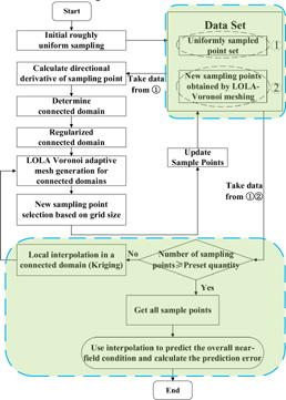
Figure 1: Process of the two-stage plane adaptive sampling algorithm.

The connected domain in Fig. 1 refers to the initial region that needs to be carefully sampled according to the gradient calculation. As can be seen from Fig. 1, the proposed sampling method mainly includes the following four steps

1) Determine the sampling surface and sampling interval according to the operating frequency and size of the device under test (DUT), and perform an initial rough uniform sampling with a larger sampling interval. Specifically determined according to the following rules [19]:

a) Sampling surface size: Make sure that the amplitude of the tangential electric field component at the edge of the sampling surface is less than 40 dB of the maximum electric field component amplitude on the entire sampling surface. In fact, this criterion is not fixed and can be adjusted appropriately according to the sampling accuracy. However, a higher threshold means larger sampling surfaces and more sampling points. Therefore, we choose 40 dB as the threshold to determine the size of the sampling surface.

b) Sampling interval: Generally speaking, there is no uniform standard to determining the sampling interval, which is often set according to the size of the sampling surface and the number of required sampling points, and is often set according to test experience. However, it should be noted that the sampling interval needs to satisfy the Nyquist spatial sampling criterion.

2) The data obtained from the initial uniform sampling is used in the optimized region self-growth algorithm to identify the central source point with drastic changes in the near field. From this source point, determine the area used for non-uniform sampling (referred to as the refinement area) and carry out reasonable regional expansion and regularization.

3) Sample the refinement area non-uniformly with the LOLA-Voronoi adaptive division method, and the sampling points are increased according to the preset number. In order to know NF information of all the sample points during the new sampling process using the LOLA-Voronoi method, the Kriging interpolation method should be used.

4) Gather the sampling point information obtained in the two stages, and use the Kriging interpolation method to restore the electromagnetic field distribution of the NF plane. Meanwhile, compare and analyze the advantages and disadvantages of the traditional dense uniform sampling method and the two-stage plane adaptive sampling algorithm in restoring the NF. Finally, calculate the relative error.

The two-stage plane adaptive sampling algorithm can densely sample in the area where the NF changes sharply, and it can roughly sample in the area where the field changes smoothly.

III. AUXILIARY SAMPLING ALGORITHM

From Section II, the core of high-efficiency and high-precision NF scanning is the two-stage plane adaptive sampling algorithm, which is mainly composed of the region self-growth optimization algorithm and the LOLA-Voronoi adaptive division algorithm. This section focuses on the two proposed algorithms, and calculates the relative error.

A. Region self-growth optimization algorithm

The proposed region self-growth algorithm for NF scanning sampling is evolved from the region growing method, which is used to segment infrared images, and its basic principle is to perform data segmentation based on the similarity of current amplitude values. In the process of determining the growing point, it is prone to getting stuck in a local optimal solution due to an unreasonable threshold setting during algorithm iteration. The innovation point of this algorithm is the optimization of the region self-growth algorithm and the way to determine the connected domain. The specific steps are as follows:

1) Determination of seed points: Solve the directional derivative of the discretized NF data obtained in the initial uniform sampling stage. The direction is from the point to be calculated to the adjacent point. For edge sampling points without adjacent points in some directions, the adjacent points in these directions are defaulted to 0. If all directional derivatives of the point to be solved are negative, the point is regarded as a seed point.

2) Region merging and regularization: First, assuming that the data obtained by NF sampling is the tangential electric field value $E$ , the adjacent points of the seed point in the $φ$ direction are denoted as $E_{φ}$ , and the ratio is calculated:

R (f) = | \frac{E - E_{f}}{E} | .

(1)

If the absolute value of the minimum value among all the ratios of the seed points is less than the parameter $d$ ( $0 < d < 1$ , $d$ directly determines the number of growing points), the adjacent points in the direction of the corresponding minimum value are taken as growing points. Second, the growing point is incorporated into the seed point set as a new seed point, and the above process is repeated until all the initial rough sampling points are traversed. Then, the connected domain will be determined according to the obtained set of seed points, that is, a new sampling area will be determined with the seed point as the center and the surrounding adjacent points as the boundary. If the determined area overlaps to form an irregular shape area, the boundary point is appropriately expanded outward to form a regular rectangular area. Its purpose is to prevent the problem of repeated sampling when using the LOLA-Voronoi adaptive division method for non-uniform sampling, and at the same time, the appropriate expansion of the area based on the seed point is conducive to restoring the area with sharp changes in the NF with higher accuracy and improving the accuracy of NF restoration.

The value of the above-mentioned parameter $d$ is usually set to 0.1 initially, and is increased in steps of 0.05 until the identified growing point no longer increases.

B. LOLA-Voronoi adaptive division method

The algorithm mainly includes two parts. One part is Voronoi tessellation, which is an intuitive method to describe the grid density. By dividing polygons, the key areas to be studied are covered as evenly as possible. The other part is LOLA, which is mainly used to evaluate the intensity of nonlinearity at each node in the key area, and then serves as the criterion for dividing the polygon density.

Voronoi tessellation method is essentially a space-filling algorithm. A group of continuous polygons is determined according to the way that one node corresponds to one Voronoi cell, and then the area size of each Voronoi cell is estimated according to the Monte Carlo method. New grid points are selected according to the area size; that is, the area size of the Voronoi cell determines the division density of the area around the node. The edge of the continuous polygon is the vertical bisector of the line segment connected by adjacent nodes. The method is shown in Fig. 2.

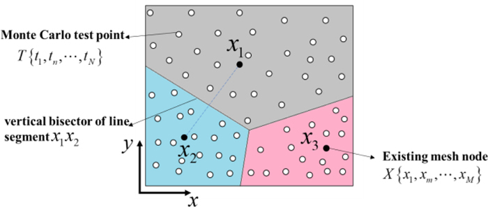
Figure 2: Voronoi schematic.

In Fig. 2, $t_{n} (n = 1, 2, \dots, N)$ represents the Monte Carlo test point, and $x_{m} (m = 1, 2, \dots, M)$ represents the existing grid node. The area of the polygon where the node $x_{1}$ is located is the largest. According to the principle of space filling of the Voronoi tessellation method, a new grid node needs to be determined in the Voronoi cell where $x_{1}$ is located.

In Fig. 2, $T {t_{1}, t_{n}, \dots, t_{N}}$ is a random, uniformly distributed Monte Carlo test point set. By filling enough test points in each Voronoi unit, the area of each irregular polygon can be estimated. For each test point, (2) needs to be satisfied:

∥ t_{n} - x_{m} ∥ \leq ∥ t_{n} - x_{m^{'}} ∥, m \neq m^{'} .

(2)

That is, to determine the Monte Carlo test point set in each Voronoi unit, it is necessary to calculate the distance between the test point $t_{n}$ and each node $x_{m}$ , and then assign the test point to the nearest node $x_{m}$ .

The Voronoi tessellation method completes the evaluation of the density of the global region, and in order to select data points according to the local characteristics of the model, the LOLA method needs to be used. The key point of LOLA is to complete the evaluation of local linear features by means of gradient estimation. The gradient $g$ at node $x_{m}$ needs to be estimated by fitting the hyperplane of $x_{m}$ and its adjacent nodes. The determination of the hyperplane requires the use of the least squares method to ensure that the fitted hyperplane can pass through the node $x_{m}$ :

\begin{matrix} (\begin{matrix} x_{m_{1}}^{(1)} - x_{m}^{(1)} & x_{m_{1}}^{(2)} - x_{m}^{(2)} & \dots & x_{m_{1}}^{(d)} - x_{m}^{(d)} \\ x_{m_{2}}^{(1)} - x_{m}^{(1)} & x_{m_{2}}^{(2)} - x_{m}^{(2)} & \dots & x_{m_{2}}^{(d)} - x_{m}^{(d)} \\ ⋮ & ⋮ & ⋮ & ⋮ \\ x_{m_{2 d}}^{(1)} - x_{m}^{(1)} & x_{m_{2 d}}^{(2)} - x_{m}^{(2)} & \dots & x_{m_{2 d}}^{(d)} - x_{m}^{(d)} \end{matrix}) \\ (\begin{matrix} g_{m}^{(1)} \\ g_{m}^{(2)} \\ ⋮ \\ g_{m}^{(d)} \end{matrix}) (\begin{matrix} f (x_{m_{1}}) \\ f (x_{m_{2}}) \\ ⋮ \\ f (x_{m_{2 d}}) \end{matrix}) \end{matrix} .

(3)

Among them, $x_{m_{i}} = (x_{m_{i}}^{(1)}, x_{m_{i}}^{(2)}, \dots, x_{m_{i}}^{(d)}) (i = 1, 2, \dots, 2 d)$ is the neighboring data point of $x_{m}$ , $f (x_{m_{i}})$ is the model output response value corresponding to the neighboring data point $x_{m_{i}}$ , $d$ is the number of dimensions, and $g = (g_{m}^{(1)}, g_{m}^{(2)}, \dots, g_{m}^{(d)})$ is the gradient matrix of each dimension.

After solving the gradient matrix $g$ , the nonlinearity near node $x_{m}$ can be obtained by using

O (x_{m}) = \sum_{i = 1}^{2 d} ∣ f (x_{m_{i}}) - (f (x_{m}) + g \cdot (x_{m_{i}} - x_{m})) ∣ .

(4)

In this way, the global region division density evaluation and the local nonlinear feature evaluation are completed, and then the two metric parameters can be comprehensively evaluated by

S (x_{m}) = V (x_{m}) + \frac{O (x_{m})}{\sum_{m - 1}^{M} O (x_{m})} .

(5)

$V (x_{m})$ represents the size of the Voronoi cell area. Bring all existing data points into (5), calculate the value of $S (x_{m})$ , and sort it. The larger the value of $S (x_{m})$ , the less dense the grid in the field. It is necessary to add new sampling points to increase the division density. Repeat the above operations to meet the preset accuracy requirements.

C. Relative error

In order to better analyze the correctness and effectiveness of the two-stage plane adaptive sampling algorithm, the relative error should be calculated as follows: First, the traditional uniform sampling and the two-stage plane adaptive sampling method are used to obtain the NF samples; then the Kriging interpolation method is used to restore the electromagnetic field distribution of the entire NF plane, and the corresponding NF value at the same position is predicted; finally, compare the predicted value with the simulated data, solve the MAPE (Mean Absolute Percentage Error) obtained by these two sampling methods respectively, and compare the relative error produced between the two methods.

M A P E = \frac{1}{n} \sum_{i = 1}^{n} | \frac{E_{o} - E_{p}}{E_{o}} | \times 100 % .

(6)

In this paper, the NF data studied are all electric field strength. Therefore, in (6), $E_{o}$ represents the actual electric field strength value obtained by electromagnetic simulation, $E_{p}$ represents the electric field strength value predicted by Kriging interpolation method, and $n$ represents the number of prediction points.

IV. EXPERIMENTS AND ANALYSIS

In order to verify the correctness and effectiveness of the proposed method, we have studied two practical cases to verify the performance of the two-stage plane adaptive sampling algorithm. Both cases are modeled and simulated by ANSYS HFSS, and the simulation results are used as the actual NF values for comparison.

A. Dipole antenna model

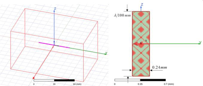
Figure 3: (a) HFSS model of half-wave dipole antenna and (b) integrated port setting method.

The first case is dipole equivalent source model, the equivalent source model commonly used in engineering, which is a simplification of the current/magnetic current source model and widely used in the field of NF analysis. The half-wave dipole is an ideal conductor material with operating wavelength $λ$ 100 mm, a total length $0.48 λ$ , and a radius $λ / 200$ . The half-wave dipole antenna is fed by a lumped port excitation method, the port size is set to $0.24 \times (λ / 100)$ mm $^{2}$ , and the distance from the radiation boundary to the antenna is $λ / 4$ , as shown in Fig. 3.

According to the implementation principle of the proposed two-stage plane adaptive sampling algorithm, in the initial rough uniform sampling of the first stage, the size of the NF sampling surface is set to $66 \times 114$ mm $^{2}$ , the sampling interval is 2 mm, and the sampling height is 1 mm. Figure 4 shows the distribution of the transient electric field amplitude $E$ of the half-wave dipole at the NF sampling plane, obtained by simulation.

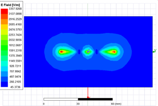
Figure 4: Distribution diagram of the transient electric field amplitude $E$ of the half-wave dipole antenna at the sampling plane.

It can be seen from Section II that the two-stage plane adaptive sampling algorithm is mainly divided into four steps. Figure 5 shows the effect diagram of the work in the four steps.

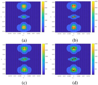
Figure 5: Dipole antenna model: (a) Step 1: Initial rough uniform sampling, (b) Step 2: Determination of the central source point, (c) Step 3: Expansion and regularization of the refinement area, and (d) Step 4: Non-uniform sampling of the refinement area.

The two-stage planar adaptive sampling algorithm first performs an initial rough uniform sampling with a sampling interval of 2 mm, and these sampling points are uniformly distributed on the entire NF sampling plane, as shown in Fig. 5 (a); secondly, the region self-growth optimization algorithm is used to identify the central source point with sharp changes in the NF, as shown in the red point in Fig. 5 (b); thirdly, the refinement area is determined based on this source point, and the reasonable area expansion and regularization are carried out, as shown in Fig. 5 (c), where the green sampling points are the boundaries; then, the LOLA-Voronoi adaptive division method is used to conduct non-uniform sampling for the refinement area, and eight sampling points are preset for each refinement area to achieve the purpose of thinning, as shown in Fig. 5 (d); finally, the information of the sampling points obtained in the two stages is summarized, and the electromagnetic distribution of the NF plane is restored using Kriging interpolation method, and the relative errors of the traditional dense uniform sampling method and the two-stage plane adaptive sampling algorithm in restoring the NF situation are calculated. Figure 6 shows a comparison of the reconstructed electric field between the two methods.

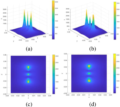
Figure 6: Dipole antenna model: (a) 3D transient electric field distribution map under uniform sampling, (b) 3D transient electric field distribution map under adaptive sampling, (c) 2D transient electric field distribution map under uniform sampling, and (d) 2D transient electric field distribution map under adaptive sampling.

It can be seen from Fig. 6 that the restored electric field distributions are well matched. After calculation, it can be seen that when the traditional dense uniform sampling method and the two-stage plane adaptive sampling method restore the NF, the relative error generated in the refinement area where the NF changes sharply is 0.0034. Meanwhile, the proposed sampling method reduces the required sampling points by 74.4% compared with the traditional uniform sampling method. Therefore, the two-stage plane adaptive sampling method is accurate and effective in terms of restoration accuracy and the number of required sampling points.

B. BGA chip model

The second case is a chip with a BGA package structure with an operating frequency of 2.5 GHz. The package of the BGA chip consists of four layers, namely the top layer, the power supply Vdd_C1 layer, the power supply Vss_C1 layer, and the bottom layer. The package size is $9.40 \times 9.40$ mm $^{2}$ and the thickness is0.73152 mm.

Two differential pairs on the chip were selected for simulation analysis. At the same time, in order to speed up the simulation, we cut the chip without affecting the simulation results, and the size after cutting is $4.70 \times 9.40$ mm $^{2}$ , as shown in Fig. 7.

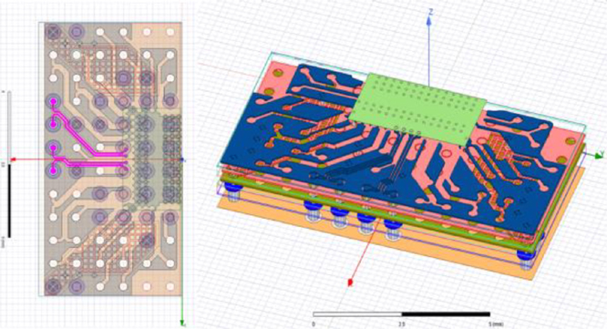
Figure 7: Two differential pair models in a BGA chip from different perspectives.

The selected two pairs of differential data lines are RXDATA3+ and RXDATA3-, and RXDATA4+ and RXDATA4-, respectively, the operating frequency is 2.5 GHz, and the power feeding is the lumped port excitation.

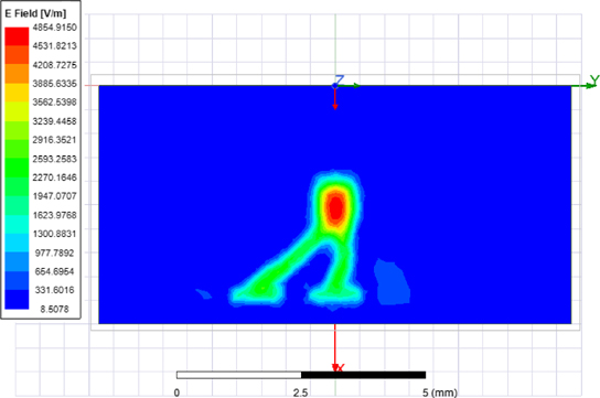
Figure 8: Distribution diagram of transient electric field amplitude of BGA chip.

The sampling surface size is set to $5 \times 9.6$ mm $^{2}$ , the sampling interval is 0.2 mm, and the NF sampling height is 0.3115 mm. The NF data is generated by ANSYS HFSS simulation. Figure 8 shows the distribution of the transient electric field amplitude of the BGA chip at the NF sampling surface. The effect diagram of the two-stage plane adaptive sampling algorithm with four steps is shown in Fig. 9.

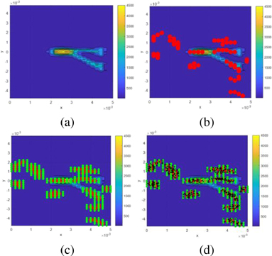
Figure 9: BGA chip model: (a) Step 1: Initial rough uniform sampling, (b) Step 2: Determination of the central source point, (c) Step 3: Expansion and regularization of the refinement area, and (d) Step 4: Non-uniform sampling of the refinement area.

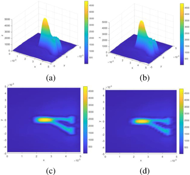
Figure 10: BGA chip model: (a) 3D transient electric field distribution map under uniform sampling, (b) 3D transient electric field distribution map under adaptive sampling, (c) 2D transient electric field distribution map under uniform sampling, and (d) 2D transient electric field distribution map under adaptive sampling.

The electromagnetic field distribution of the NF plane is restored by the two methods shown in Fig. 10, including a three-dimensional instantaneous electric field comparative analysis diagram and a two-dimensional plane instantaneous electric field comparative analysis diagram.

It can be seen from Fig. 10 that the restored electric field distributions are well matched. After calculation, it can be seen that when the two sampling methods restore the NF, the relative error generated in the refinement area where the NF changes sharply is 0.0698. Meanwhile, the number of sampling points required by the two-stage plane adaptive sampling method is decreased by 74.2%. Therefore, compared with the traditional uniform sampling method, the proposed sampling method is more accurate and effective from the perspective of restoration accuracy and the number of required sampling points.

The number of NF samples required to use the two-stage planar adaptive sampling algorithm is smaller when the NF accuracy is similar. Compared with the traditional uniform sampling method, when the proposed sampling method samples the half-wave dipole module and the BGA chip module, the number of required NF samples is reduced by 74.4% and 74.2%, respectively. Therefore, the proposed sampling method can effectively reduce the number of required NF samples while ensuring the restoration accuracy.

V. CONCLUSION

In this paper, a two-stage plane adaptive NF scanning algorithm is proposed, which solves the problem of long acquisition time of NF data in the NF scanning process, and can efficiently image the radiation source in the high-speed integrated circuit board. Based on the region self-growth optimization algorithm and the Voronoi subdivision principle, the method significantly reduces the number of NF scanning points required to characterize the electromagnetic behavior of the DUT by means of uniform and non-uniform two-stage sampling, and reconstructs the NF electromagnetic distribution of the DUT with high resolution by means of Kriging interpolation.

By studying the specific performance of the new method in the application of NF scanning, this paper proves the correctness and effectiveness of the two-stage plane adaptive scanning algorithm in determining multiple strong radiation sources and accurately restoring the NF distribution of the DUT. The dominant advantage of the method proposed in this paper is to significantly reduce the number of NF samples by nearly 75% in near-field scanning. Therefore, it would be widely applied in evaluating the EMC characteristics of integrated circuits, locating EMI sources, and efficiently completing the reconstruction of radiationsources.

Footnote

Supported by Beijing Natural Science Foundation.

REFERENCES

[1] A. Taaghol and T. Sarkar, “Near-field to near/far-field transformation for arbitrary near-field geometry, utilizing an equivalent magnetic current,” IEEE Trans. Electromagn. Compat., vol. 38, no. 3, pp. 536-542, 1996.

[2] T. Sarkar and A. Taaghol, “Near-field to near/far-field transformation for arbitrary near-field geometry utilizing an equivalent electric current and mom,” IEEE Trans. Antennas Propag., vol. 47, no. 3, pp. 566-573, 1999.

[3] Y. Alvarez Lopez, F. Las-Heras Andres, M. R. Pino, and T. K. Sarkar, “An improved super-resolution source reconstruction method,” IEEE Trans. Instrum. Meas., vol. 58, no. 11, pp. 3855-3866, 2009.

[4] P. Li and L. J. Jiang, “A rigorous approach for the radiated emission characterization based on the spherical magnetic field scanning,” IEEE Trans. Electromagn. Compat., vol. 56, no. 3, pp. 683-690, 2014.

[5] H. Wang, V. Khilkevich, Y.-J. Zhang, and J. Fan, “Estimating radiofrequency interference to an antenna due to near-field coupling using decomposition method based on reciprocity,” IEEE Trans. Electromagn. Compat., vol. 55, no. 6, pp. 1125-1131, 2013.

[6] J. Zhang and J. Fan, “Source reconstruction for IC radiated emissions based on magnitude-only near-field scanning,” IEEE Trans. Electromagn. Compat., vol. 59, no. 2, pp. 557-566, 2017.

[7] W.-J. Zhao, E.-X. Liu, B. Wang, S.-P. Gao, and C. E. Png, “Differential evolutionary optimization of an equivalent dipole model for electromagnetic emission analysis,” IEEE Trans. Electromagn. Compat., vol. 60, no. 6, pp. 1635-1639, 2018.

[8] Y.-F. Shu, X.-C. Wei, R. Yang, and E.-X. Liu, “An iterative approach for EMI source reconstruction based on phaseless and single-plane near-field scanning,” IEEE Trans. Electromagn. Compat., vol. 60, no. 4, pp. 937-944, 2018.

[9] J.-C. Zhang, X. Wei, L. Ding, X.-K. Gao, and Z.-X. Xu, “An EM imaging method based on plane-wave spectrum and transmission line model,” IEEE Trans. Microw. Theory Tech., vol. 68, no. 10, pp. 4161-4168, 2020.

[10] A. Tankielun, H. Garbe, and J. Werner, “Calibration of electric probes for post-processing of near-field scanning data,” Proc. IEEE Int. Symp. Electromagn. Compat., vol. 1, pp. 119-124, Aug.2006.

[11] M. R. Ramzi, M. Abou-Khousa, and I. Prayudi, “Near-field microwave imaging using open-ended circular waveguide probes,” IEEE Sensors J., vol. 17, no. 8, pp. 2359-2366, 2017.

[12] S. Jarrix, T. Dubois, R. Adam, P. Nouvel, B. Azais, and D. Gasquet, “Probe characterization for electromagnetic near-field studies,” IEEE Trans. Instrum. Meas., vol. 59, no. 2, pp. 292-300,2010.

[13] H. Weng, D. G. Beetner, and R. E. DuBroff, “Frequency-domain probe characterization and compensation using reciprocity,” IEEE Trans. Electromagn. Compat., vol. 53, no. 1, pp. 2-10,2011.

[14] D. Deschrijver, F. Vanhee, D. Pissoort, and T. Dhaene, “Automated nearfield scanning algorithm for the EMC analysis of electronic devices,” IEEE Trans. Electromagn. Compat., vol. 54, no. 3, pp. 502-510, 2012.

[15] P. Singh, D. Deschrijver, D. Pissoort, and T. Dhaene, “Accurate hotspot localization by sampling the near-field pattern of electronic devices,” IEEE Trans. Electromagn. Compat., vol. 55, no. 6, pp. 1365-1368, 2013.

[16] P. Singh, T. Claeys, G. A. E. Vandenbosch, and D. Pissoort, “Automated line-based sequential sampling and modeling algorithm for EMC near-field scanning,” IEEE Trans. Electromagn. Compat., vol. 59, no. 2, pp. 704-709, 2017.

[17] R. Brahimi, A. Kornaga, M. Bensetti, D. Baudry, Z. Riah, A. Louis, and B. Mazari, “Postprocessing of near-field measurement based on neural networks,” IEEE Trans. Instrum. Meas., vol. 60, no. 2, pp. 539-546, 2011.

[18] Y.-R. Feng, X.-C. Wei, L. Ding, T.-H. Song, R. X.-K. Gao, “A hybrid schatten p-norm and lp-norm with plane wave expansion method for near-near field transformation,” IEEE Trans. Electromagn. Compat., vol. 63, no. 6, pp. 2074-2081,2021.

[19] S. Tao, H. Zhao, and Z. D. Chen, “An adaptive sampling strategy based on region growing for near-field-based imaging of radiation sources,” IEEE Access, vol. 9, pp. 9550-9556, 2021.

[20] S. Serpaud, A. Boyer, S. Ben-Dhia, and F. Coccetti, “Fast and accurate near-field measurement method using sequential spatial adaptive sampling (SSAS) algorithm,” IEEE Trans. Electromagn. Compat., vol. 63, no. 3, pp. 858-869, 2021.

[21] J.-R. Regue, M. Ribo, J.-M. Garrell, and A. Martin, “A genetic algorithm based method for source identification and far-field radiated emissions prediction from near-field measurements for PCB characterization,” IEEE Trans. Electromagn. Compat., vol. 43, no. 4, pp. 520-530, 2001.

[22] W.-J. Zhao, B.-F. Wang, E.-X. Liu, H. B. Park, H. H. Park, E. Song, and E.-P. Li, “An effective and efficient approach for radiated emission prediction based on amplitude-only near-field measurements,” IEEE Trans. Electromagn. Compat., vol. 54, no. 5, pp. 1186-1189, 2012.

[23] F.-P. Xiang, E.-P. Li, X.-C. Wei, and J.-M. Jin, “A particle swarm optimization-based approach for predicting maximum radiated emission from PCBs with dominant radiators,” IEEE Trans. Electromagn. Compat., vol. 57, no. 5, pp. 1197-1205, 2015.

[24] J. A. Russer, N. Uddin, A. S. Awny, A. Thiede, and P. Russer, “Nearfield measurement of stochastic electromagnetic fields,” IEEE Electromagn. Compat. Mag., vol. 4, no. 3, pp. 79-85, 2015.

[25] E. X. Liu, W. J. Zhao, B. F. Wang, and X. C. Wei, “Near-field scanning and its EMC applications,” Proc. Int. Symp. IEEE Electromagn. Compat., pp. 937-944, 2017.

[26] H. P. Zhao, S. H. Tao, Z. Z. Chen, and J. Fan, “Sparse source model for prediction of radiations by transmission lines on a ground plane using a small number of near-field samples,” IEEE Antennas Wireless Propag. Lett., vol. 18, no. 1, pp. 103-107, Jan. 2019.

[27] N. A. Abou-Khousa and A. Haryono, “Array of planar resonator probes for rapid near-field microwave imaging,” IEEE Trans. Instrum. Meas., vol. 69, no. 6, pp. 3838-3846, June 2020.

[28] K. Crombecq, D. Gorissen, D. Deschrijver, and T. Dhaene, “A novel hybrid sequential design strategy for global surrogate modeling of computer experiments,” SIAM J. Sci. Comput., vol. 33, no. 4, pp. 1948-1974, Jan. 2011.

[29] J. Tao, W. Tang, B. Li, S. Zhang, and R. Sun, “Efficient indoor signal propagation model based on LOLA-Voronoi adaptive meshing,” Applied Computational Electromagnetics (ACES) Society Journal, vol. 35, no. 4, pp. 437-442, 2020.

[30] S. Huang, Z. Peng, Z. Wang, X. Wang, and M. Li, “Infrared small target detection by density peaks searching and maximum-gray region growing,” IEEE Geosci. Remote Sens. Lett., vol. 16, no. 12, pp. 1919-1923, Dec. 2019.

BIOGRAPHIES

Xiaoyong Liu received the bachelor’s degree in radio technology and information system from Tsinghua University, Beijing, China, in 2002. He is currently working toward the doctor’s degree in electronic science and technology from the Beijing University of Posts & Telecommunications, Beijing, China. His research interests include electromagnetic compatibility, testing and measurement, radio frequency spectrum technology.

Peng Zhang received the bachelor’s degree in electronic engineering from Nanjing Institute of Technology, Nanjing, China, in 2020. He is currently working toward the master’s degree in electronics and communication engineering from the Beijing University of Posts & Telecommunications, Beijing, China. His research interests include chip electromagnetic compatibility and reconstruction of emission sources.

Dan Shi (M’08) received the Ph.D. degree in electronic engineering from Beijing University of Posts & Telecommunications, Beijing, China, in 2008. She has been a professor in Beijing University of Posts & Telecommunications. Her interests include electromagnetic compatibility, electromagnetic environment, and electromagnetic computation.