Resonant Frequency Modelling of Microstrip Antennas by Consensus Network and Student’s-T Process
Xuefeng Ren, Yubo Tian, Qing Li, and Hao Fu
1Ocean College Jiangsu University of Science and Technology, Zhenjiang, 212100, China
211110302104@stu.just.edu.cn
2School of Information and Communication Engineering Guangzhou Maritime University, Guangzhou 510725, Guangdong, China
tianyubo@just.edu.cn
3Ocean College Jiangsu University of Science and Technology, Zhenjiang, 212100, China
leo199808@163.com
4Ocean College Jiangsu University of Science and Technology, Zhenjiang, 212100, China
2841689068@qq.com
Submitted On: July 5, 2023; Accepted On: January 25, 2024
ABSTRACT
When modelling and optimizing antennas by machine learning (ML) methods, it is the most time-consuming to obtain the training samples with labels from full-wave electromagnetic simulation software. To address the problem, this paper proposes an optimization method based on the consensus results of multiple independently trained Student’s-T Process (STP) with excellent generalization ability. First, the STP is introduced as a surrogate model to replace the traditional Gaussian Process (GP), and the hyperparameters of the STP model are optimized. Afterwards, a consistency algorithm is used to process the results of multiple independently trained STPs to improve the reliability of the results. Furthermore, an aggregation algorithm is adopted to reduce the error obtained in the consistency results if it is greater than the consistency flag. The effectiveness of the proposed model is demonstrated through experiments with rectangular microstrip antennas (RMSA) and circular microstrip antennas (CMSA). The experimental results show that the use of multiple independently trained STPs can accelerate the antenna design optimization process, and improve modelling accuracy while maintaining modelling efficiency, which has high generalization ability.
Index Terms: Antenna optimization, Consensus network, Gaussian Process, Student’s-T Process.
I. INTRODUCTION
In the past research, the optimal design of electromagnetic (EM) components has often relied on numerical simulation or full-wave EM simulation software, such as High-Frequency Structure Simulator (HFSS), Computer Simulation Technique (CST), and combined with global optimization algorithms [1, 2] to perform research experiments with significant results. Although these numerical simulation tools can provide high fidelity simulation results, the process of evaluating the performance of EM components requires multiple calls to the EM simulation software, and each calculation is time-consuming and inefficient. As a result, the focus of current research has shifted to the surrogates of EM simulation software to assess the suitability of EM components. The introduction of surrogates offers the advantage of saving time and resources, especially for the more complex EM components. Surrogates are approximate models that allow predictions and evaluations in a short time by analyzing and modelling a small amount of EM simulation data, thereby improving computational efficiency while maintaining some accuracy. Some modelling methods such as Artificial Neural Networks (ANN) [3, 4, 5], Support Vector Machines (SVM) [6, 7], Extreme Learning Machines (ELM) [8, 9, 10], Gaussian Processes (GP) [11, 12, 13] and Backpropagation (BP) [14] are currently in use and can effectively solve electromagneticproblems.
ANN has a powerful self-learning capability to handle complex problems, but it requires a large amount of simulation data, and determining its structure is very difficult. SVM has good generalization ability and is suitable for small samples, which can effectively avoid ”dimensional disaster” due to its final decision function, but the predicted output is not probabilistic and its kernel parameters are difficult to determine. As a classical surrogate, GP can not only face complex mathematical problems, but also solve mathematical problems in high-dimensional space, and its mathematical theoretical foundation is more rigorous [15]. However, the posterior distribution of the GP always depends on the observations, and its outliers are a preferential assumption, leading to extreme outlier observations that cannot effectively be ignored [16]. The Student’s-T Process (STP) obeys the Student’s-T distribution rather than the Gaussian distribution, it has a more flexible posterior variance and more robust performance compared to the GP. Shah et al. obtained the closed expressions for the marginal likelihood and predictive distribution of the STP by inverting the Wishart integral process over the covariance kernel of the GP model, and it was shown that the STP not only retains the properties of the non-parametric representation of the GP but also has greater flexibility concerning the predicted covariance [17]. Sloin and Särkkä added a noise covariance function to the parametric kernel to construct the STP, and used it as an alternative to GP, which can make the computation more concise [18]. Tang et al. proposed STP with the Student’s-T likelihood for dealing with input and target outliers [19]. Chen et al. constructed a unified framework to derive a multivariate STP model, which not only addressed some of the shortcomings of existing methods in solving multiple output prediction problems but was also more effective compared to the traditionalGP [20].
As a Machine Learning (ML) technique, STP is easy to implement with few parameters in the learning process, achieves better results in solving non-linear, high-dimensional problems with small sample sizes, and the final result has probabilistic significance [21]. STP can effectively map the non-linear functional dependencies between the input and output, and become a valuable tool for the modelling and optimization of complex EM problems. However, sometimes, the accuracy and reliability of STP results remain problematic. Even after adequate training, the predicted results of STP still have errors that cannot be neglected compared with ones obtained by full-wave EM simulation software. When STP is used to optimally design an antenna, these deviations can temporarily or permanently lead the optimization in the wrong direction, thereby prolonging the optimization time or rendering the antenna design infeasible.
This paper proposes a generic method for the optimal design of antennas, reducing the uncertainty of the results obtained from a single STP. It is based on consensus results from multiple independently trained STPs. First, STP is introduced as a surrogate to replace the conventional GP and its hyperparameters are optimized. Then, a consensus algorithm is used to process the results of multiple independently trained STPs to improve the reliability of the results. Moreover, an aggregation algorithm is adopted to reduce the error of the consensus results if it is greater than the consistency flag.
The rest of this paper is structured as follows. The second part gives a brief description of GP and STP. The third part details the basic principles, model structure and algorithm flowchart and pseudo-code of the consistency-based STP model. The fourth part is the experiments, including the resonant frequencies of rectangular microstrip antennas (RMSA) and circular microstrip antennas (CMSA), and the modelling results of different methods show that the proposed consensus STP network, named C-STP, is more effective. The last part is the conclusion and outlook.
II. BACKGROUND INFORMATION
A. Gaussian process
GP is a powerful ML method, which can be determined only by the mean function and covariance function, as shown in equation (1):
| (1) |
In the above formula, are any random variables, is the mean value function, and is the covariance function. GP can be further expressed by the following equation [22]:
| (2) |
If there are observations in the training set ,is a -dimensional input training matrix with d-dimensional input training vectors. is a training output vector with training output scalar .If there is noise , the regression model can be expressed as , where is a random variable obeying a normal distribution with a mean of 0 and a variance of , which can be expressed as:
| (3) |
Then the prior distribution of the observed target value is as follow:
| (4) |
where is a symmetric positive definite covariance matrix of order , and is the identity matrix. Outputs of training samples and of test samples forms a joint Gaussian prior distribution, which can be expressed as:
| (5) |
In the above equation, is the order covariance matrix between test samples and training samples, and is the order covariance matrix of test samples.
Typically, the covariance matrix of GP regression model, also known as kernel function, is chosen from the Automatic Relevance Determination (ARD) series of squared exponential kernels, which contain a set of hyperparameters that determine the nature of the GP model. In the actual modelling process, the hyperparameters of the GP model are determined through calculating the maximum likelihood function. First, the conditional probabilities of the log marginal likelihood functions of the training samples are constructed, and then the bias derivatives of the hyperparameters contained therein are obtained. Finally, the hyperparameters are optimized using a conjugate gradient optimization method to find the optimal solution. The expression for the negative log-likelihood function is given by:
| (6) |
After the optimal value of the hyperparameter is obtained, the trained GP is used for predictions.
Given a new set of data input , based on the trained GP model with the training set , the posterior distribution of the predicted value of the new input can be written:
| (7) |
where formula (8) is the predicted mean value matrix, and formula (9) is the predicted covariance matrix:
| (8) |
| (9) |
Through the above series of calculations, the GP can predict the output corresponding to the .
B. Student’s-T process
STP is a function distribution of an infinite set of random variables subject to multivariate Student’s-T distribution, which is an extension of GP. We describe the Student’s-T distribution in this way [23]:
| (10) | ||
In the above equation, is the dimension of the Student’s-T distribution, is the mean vector, is the correlation matrix, is the degree of freedom and :
| (11) |
STP includes mean function , kernel function and degree of freedom , and they also determine STP properties. If is any random variable, STP can be given by:
| (12) |
If the degrees of freedom increase infinitely and finally converge to infinity, the multivariate Student’s-T distribution will become a multivariate Gaussian distribution, which has the same mean and correlation function.
In STP, the prior expected value of each position is defined by the mean function .The covariance between the values of and at any two positions is represented by the kernel function, and then the joint probability distribution of a finite subset of positions can be expressed as:
| (13) |
In the above equation, represents means vector, £ is the degree of freedom, is the kernel matrix .
Given a set of samples , a posteriori of STP is given by:
| (14) |
where
| (15) |
| (16) |
| (17) |
Generally, the kernel of the square index is selected as kernel function [24]and is given by:
| (18) |
where is the signal variance and can also be the output scale amplitude, and the parameter is the input (length or time) scale.
The combination of equation (14) and the kernel function shows that the posterior covariance of STP is dependent on not only the test observations but also the training observations [25]. Therefore, as a surrogate model, STP has more flexible post-verification difference. In addition, using the same method as the GP, its hyperparameter can be estimated by the maximum marginal likelihood. The form of its negative logarithmic likelihood function can be given by:
| (19) |
III. THE PROPOSED MODEL
The consensus STP, named C-STP, is proposed in this paper, as shown in Fig. 1, which is constructed by multiple individual STPs that map the physical parameter of an antenna to the output parameter , such as resonant frequency. The nonlinear transform , where implements the mapping, where is the length of .
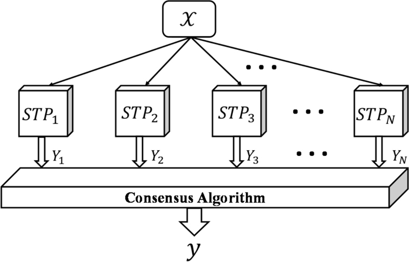
Figure 1: Structure diagram of consistent Student’s-T Process model.
For the STP used in this paper, the ARD series square index kernel (20) is selected, and the hyperparameter is optimized through nonlinear optimization method. STP’s degree of freedom , noise variance , signal variance , and kernel function hyperparameter are all targets that need to be optimized. The optimization process is shown in Fig. 2. Taking the negative log-marginal likelihood function of STP as the objective function, gradient-based numerical optimization techniques including the conjugate gradient method or other intelligent optimization algorithms are used to calculate the minimum value of the negative log-marginal likelihood function and obtain the final hyperparameter. When a new observation is given, the output can be accurately predicted:
| (20) |
where is the element component , which represents the length scale of each corresponding input dimension.
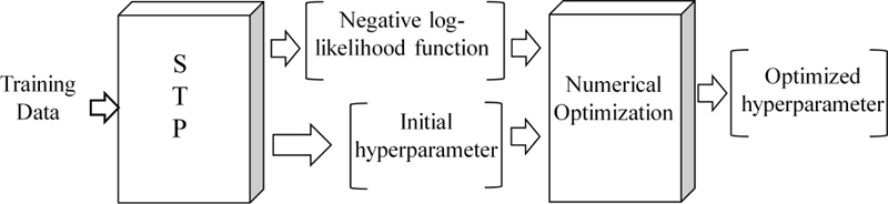
Figure 2: STP hyperparameter optimization flow chart.
A. Consensus of STP
Training STP to predict as accurately as possible for any input requires non-linear optimization method to find the minimum value of the negative log marginal likelihood function and determines the value of the hyperparameter. The training process can start with random values of the hyperparameter or some predefined values. These values, along with the optimization algorithm used to adjust the hyperparameters, determine the final STP. If a random method is used, the final result is random, that is, each training will produce a slightly different STP instance. In theory, training might produce the same STP, but we don’t observe it in the experiments.
If only one STP is trained for antenna frequency modelling, even if it is well trained, its output results may have uncertainties related to the STP training. The effectiveness of the trained STP result depends on its kernel functions, hyperparameters, training programs and data set. To improve the effectiveness of independently trained STP results and make them more accurate, we use multiple STP instances instead of one STP, as shown in Fig. 1. This topology is called consensus STP, referred to as C-STP in this paper, and similar methods have been used in previous studies in medicine, EM and computer science [26, 27, 28]. The core idea of consensus STP is to use multiple STPs simultaneously by providing an identical training task to each STP separately. If the input is same for all STPs, then the consensus algorithm is performed for the output of all STPs, i.e. , where is the total number of STPs. The consensus module can give the final output as shown in Fig. 1, and the threshold determines whether all the results are consistent. Usually, and can be either real set of data, which is common in antenna design, or discrete set data, and the C-STP can be used for both types of data. There are some methods to implement the consensus algorithm, including majority voting, arithmetic or other mean algorithms. The decision is mostly influenced by the tasks specifications and the outputs characteristics.
The training process of multiple STPs can be performed in parallel because all STPs are independent of each other, and there is no data exchange. Therefore, the C-STP approach is well suited for applications on multi-core computing architectures. Typically, the STPs may have the same or different kernel functions and hyperparameters, but all STPs must perform the same training task.
B. Consensus algorithm
In the whole work, we use multiple training sets to train STP randomly. The training process is repeated for times, therefore different STPs can be generated. The consistency algorithm is to calculate the arithmetic mean from the output of all the STPs.
| (21) |
we can find the output that deviates the most from , i.e.
| (22) |
Then we exclude the output of the STP and calculate the arithmetic mean of all other STPs as:
| (23) |
In addition, for each pair of STP outputs, and , and , if (24) is satisfied, we believe that the two STPs are consistent.
| (24) |
where is a pre-defined threshold. In this case, it is the final output of the C-STP. Otherwise, it is no consensus, and the C-STP cannot predict the output correctly. In this case, the output is computed by other methods. In general, the is set according to the problem we are facing, and it is different depending on the problem.
When it is no consensus, we adopt the aggregation method proposed by Goel et al. [29] to construct the final result. This method is simple in operation and has good usability, especially with high modelling efficiency. The weight factor solution method of each model is as follows:
| (25) |
| (26) |
The parameters and are used to measure the importance of the average model and a single approximate model. Experiments show that can obtain an accurate consensus model for most problems. is the global error of the approximate model, and the value can be determined by the specific error index used.
The consensus algorithm allows a STP to predict the output inaccurately, while the proposed C-STP can give a more accurate output because the algorithm eliminates the worst predictions. On the flip side, if the outputs of all STPs predictions are within , excluding one result does not affect the final output. Therefore, compared with the simple arithmetic mean of independent STP output, the consistency algorithm is more accurate. The proposed consensus algorithm meets .
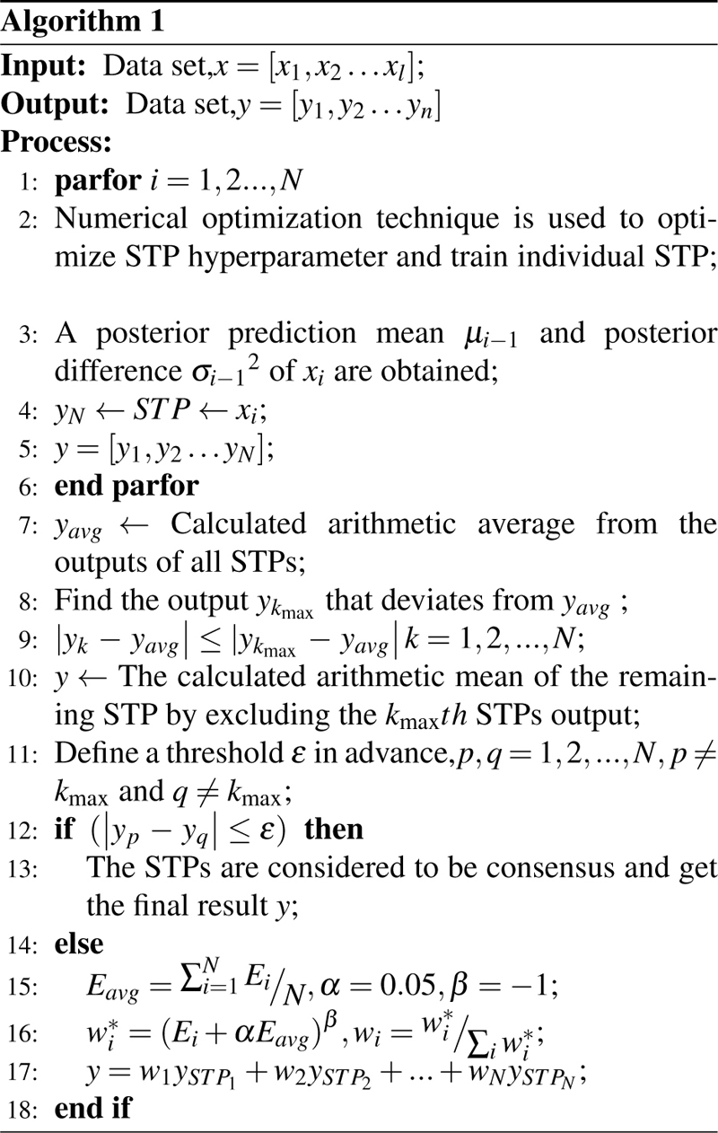
The pseudo-program code for the proposed algorithm is shown in Algorithm 1.
IV. EXPERIMENTS
A. Single STP regression
First, a single STP is trained and tested. Ten regression data sets are selected from the database [30] of the University of California, Irvine (UCI). These data sets have different capacities, which can verify the effectiveness of STP. Experimental results from STP and related parameters for these 10 regression problems are shown in Table 1, Table 2 and Fig. 3. The results obtained by SVM [31], Least Squares Support Vector Machine (LSSVM) [32], ELM [33], GP [34] and other classical models are selected to compare with STP, verifying the effectiveness of the STP. Root mean square error (RMSE) is adopted as the performance evaluation index to measure the prediction error of different models. Table 2 shows the prediction results of each model, and the best ones for different problems are shown in bold.
| (27) |
where is the real value, is the predicted value, and is the total number of samples.
| Data | Train Samples | Test Samples | Input Feature |
| Strike | 416 | 209 | 6 |
| Pyrim | 49 | 25 | 27 |
| Housing | 337 | 169 | 13 |
| Weather Izmir | 974 | 487 | 9 |
| Abalone | 2784 | 1393 | 8 |
| Quake | 1452 | 726 | 3 |
| Cleveland | 202 | 101 | 13 |
| Mortgage | 699 | 350 | 15 |
| Bodyfat | 168 | 84 | 14 |
| Basketball | 64 | 32 | 4 |
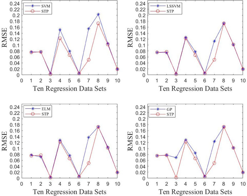
Figure 3: Comparison of different models with STP.
Table 2: Error of different models
| Data Set | SVM | LSSVM | ELM | GP | STP |
| Strike | 0.1053 | 0.1007 | 0.1043 | 0.1023 | 0.1020 |
| Pyrim | 0.15497 | 0.1133 | 0.1376 | 0.1236 | 0.0507 |
| Housing | 0.0792 | 0.0780 | 0.0762 | 0.0849 | 0.0663 |
| Weather Izmir | 0.0190 | 0.0191 | 0.0191 | 0.0194 | 0.0193 |
| Abalone | 0.0773 | 0.0756 | 0.0777 | 0.0758 | 0.0756 |
| Quake | 0.2029 | 0.1733 | 0.1729 | 0.1728 | 0.1728 |
| Cleveland | 0.1514 | 0.1256 | 0.1281 | 0.1293 | 0.1227 |
| Mortgage | 0.0049 | 0.0053 | 0.0057 | 0.0056 | 0.0048 |
| Bodyfat | 0.0049 | 0.0038 | 0.0033 | 0.0690 | 0.0020 |
| Basketball | 0.0767 | 0.0744 | 0.0719 | 0.0776 | 0.0772 |
It can be seen that the STP used in this paper outperforms other models in at least 7 out of 10 datasets. Moreover, it outperforms anyone of the classical models in at least 9 out of 10 datasets. Therefore, the STP has good predictive ability.
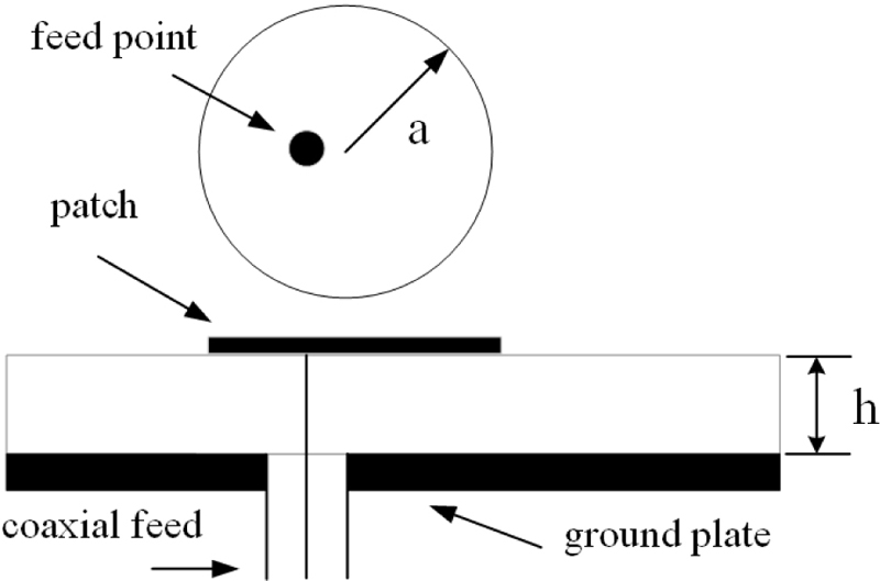
Figure 4: Schematic diagram of the CMSA.
B. Antennas resonant frequency
To gain insight into the performance of the proposed C-STP and demonstrate its effectiveness, we generate 10 STPs for the following experiments. Since there are multiple groups of data in the test set, each STP prediction output will also have multiple groups. In order to unify the calculation, we use the average difference between the predicted result and the true value as output, so that each STP will only have one predicted result, and then it is compared in pairs to compute the consistency. From several experiments, the threshold setting for CMSA and for RMSA are considered reasonable. Of course, the number of STPs in the C-STP as well as the threshold are determined according to the problem.
The CMSA [35] selected in this paper is shown in Fig. 4, and the proposed C-STP is used to predict its resonant frequency. The input variables of the CMSA are , , , where is the radius of the circular patch, is the thickness of the dielectric layer, and is the relative dielectric constant, and the output is the resonant frequency corresponding to each group of samples. There are 20 groups of experimental data, among which 16 groups are selected as the training set, and the remaining 4 groups labelled with * symbol are selected as the test set, as shown in Table 3. At the same time, we also select four different modelling methods, including BP, SVM, GP and STP, to compare with the proposed C-STP. The test results are shown in Table 4 and Fig. 5. The evaluation metric is the average percentage error (APE), i.e.
| (28) |
where is the real value, is the predicted value, and is the total number of samples.
Table 3: Samples of the CMSA for the proposed C-STP method
| Number | a/cm | h/cm | f/MHz | |
| 1* | 6.8 | 0.08 | 2.32 | 835 |
| 2 | 6.8 | 0.159 | 2.32 | 829 |
| 3 | 2 | 0.2350 | 4.55 | 2003 |
| 4 | 5 | 0.159 | 2.32 | 1128 |
| 5 | 3.8 | 0.1524 | 2.49 | 1443 |
| 6 | 4.85 | 0.318 | 2.52 | 1099 |
| 7* | 3.493 | 0.3175 | 2.5 | 1510 |
| 8 | 1.27 | 0.0794 | 2.59 | 4070 |
| 9 | 3.493 | 0.1588 | 2.5 | 1570 |
| 10 | 4.95 | 0.235 | 4.55 | 825 |
| 11 | 3.975 | 0.235 | 4.55 | 1030 |
| 12 | 2.99 | 0.235 | 4.55 | 1360 |
| 13* | 6.8 | 0.318 | 2.32 | 815 |
| 14 | 1.04 | 0.235 | 4.55 | 3750 |
| 15 | 0.77 | 0.235 | 4.55 | 4945 |
| 16 | 1.15 | 0.15875 | 2.65 | 4425 |
| 17 | 1.07 | 0.15875 | 2.65 | 4723 |
| 18 | 0.96 | 0.15875 | 2.65 | 5524 |
| 19 | 0.74 | 0.15875 | 2.65 | 6634 |
| 20* | 0.82 | 0.15875 | 2.65 | 6074 |
Table 4: Test results of different methods for the CMSA
| f/MHz | BP | SVM | GP | STP | Proposed |
| 835 | 618 | 837.6 | 825.4 | 829.7 | 829 |
| 1510 | 1313 | 1462.7 | 1547.2 | 1553.8 | 1549 |
| 815 | 831.9 | 779.9 | 814.6 | 829 | 829 |
| 6074 | 6018 | 6136.4 | 6297.9 | 6297.9 | 6155.9 |
| APE(%) | 10.3012 | 2.2629 | 1.8340 | 1.6718 | 1.5498 |
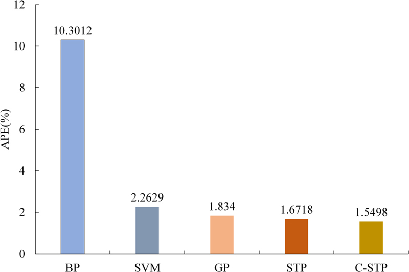
Figure 5: APE of different models for the CMSA.
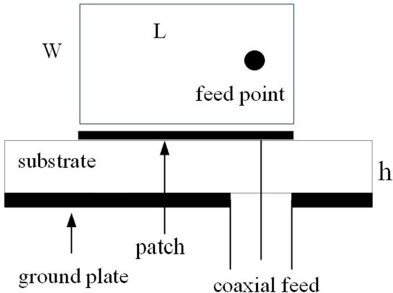
Figure 6: Schematic diagram of the RMSA.
Table 5: Samples of the RMSA for the proposed C-STP method
| Number | W/cm | L/cm | h/cm | f/MHz | |
| 1* | 0.790 | 1.185 | 0.017 | 2.22 | 8450 |
| 2 | 0.910 | 1.000 | 0.127 | 10.20 | 4600 |
| 3 | 2.000 | 2.500 | 0.079 | 2.22 | 3970 |
| 4 | 0.850 | 1.290 | 0.017 | 2.22 | 7740 |
| 5 | 1.063 | 1.183 | 0.079 | 2.25 | 7730 |
| 6* | 1.810 | 1.960 | 0.157 | 2.33 | 4805 |
| 7 | 1.720 | 1.860 | 0.157 | 2.33 | 5060 |
| 8 | 1.170 | 1.280 | 0.300 | 2.50 | 6570 |
| 9 | 0.987 | 1.450 | 0.450 | 2.55 | 6070 |
| 10 | 0.776 | 1.080 | 0.330 | 2.55 | 8000 |
| 11 | 0.790 | 1.620 | 0.550 | 2.55 | 5990 |
| 12* | 1.337 | 1.412 | 0.200 | 2.55 | 5800 |
| 13 | 0.905 | 1.018 | 0.300 | 2.50 | 7990 |
| 14 | 1.500 | 1.621 | 0.163 | 2.55 | 5600 |
| 15 | 1.120 | 1.200 | 0.242 | 2.55 | 7050 |
| 16 | 1.530 | 1.630 | 0.300 | 2.50 | 5270 |
| 17 | 1.270 | 1.350 | 0.163 | 2.55 | 6560 |
| 18* | 1.375 | 1.580 | 0.476 | 2.55 | 5100 |
| 19 | 0.814 | 1.440 | 0.476 | 2.55 | 6380 |
| 20 | 1.403 | 1.485 | 0.252 | 2.55 | 5800 |
| 21 | 0.790 | 1.255 | 0.400 | 2.55 | 7134 |
| 22 | 0.783 | 2.300 | 0.854 | 2.55 | 4600 |
| 23* | 1.000 | 1.520 | 0.476 | 2.55 | 5820 |
| 24 | 0.883 | 2.676 | 1.000 | 2.55 | 3980 |
| 25 | 1.265 | 3.500 | 1.281 | 2.55 | 2980 |
| 26 | 1.200 | 1.970 | 0.626 | 2.55 | 4660 |
| 27 | 0.974 | 2.620 | 0.952 | 2.55 | 3980 |
| 28 | 0.920 | 3.130 | 1.200 | 2.55 | 3470 |
| 29* | 1.256 | 2.756 | 0.952 | 2.55 | 3580 |
| 30 | 1.080 | 3.400 | 1.281 | 2.55 | 3150 |
| 31 | 1.020 | 2.640 | 0.952 | 2.55 | 3900 |
| 32 | 0.777 | 2.835 | 1.100 | 2.55 | 3900 |
| 33* | 1.030 | 3.380 | 1.281 | 2.55 | 3200 |
Table 6: Test results of different methods for the RMSA
| /GHz | DBD | BP | EDBD | PTS | GP | STP | Proposed |
| 8450 | 8226 | 8233.1 | 8328.2 | 8148.6 | 8041 | 8289.1 | 8290.2 |
| 4805 | 4684.8 | 4703.3 | 4699.2 | 4879 | 4807 | 4860.3 | 4861.5 |
| 6200 | 6142.6 | 6147.2 | 6176.6 | 6205.7 | 6164 | 6192.3 | 6191.5 |
| 5100 | 5293.2 | 5291.4 | 5311.8 | 5191.4 | 5112 | 5047.2 | 5076.5 |
| 5820 | 5918 | 5924.5 | 5931 | 5780.3 | 5876 | 5865.7 | 5868.5 |
| 3580 | 3655.7 | 3644.6 | 3659.8 | 3685.2 | 3590 | 3578.5 | 3582.4 |
| 3200 | 3184.7 | 3178 | 3230.3 | 3167 | 3183 | 3206.4 | 3205.7 |
| APE (%) | 2.020 | 1.939 | 1.894 | 1.663 | 1.0716 | 0.7559 | 0.6778 |
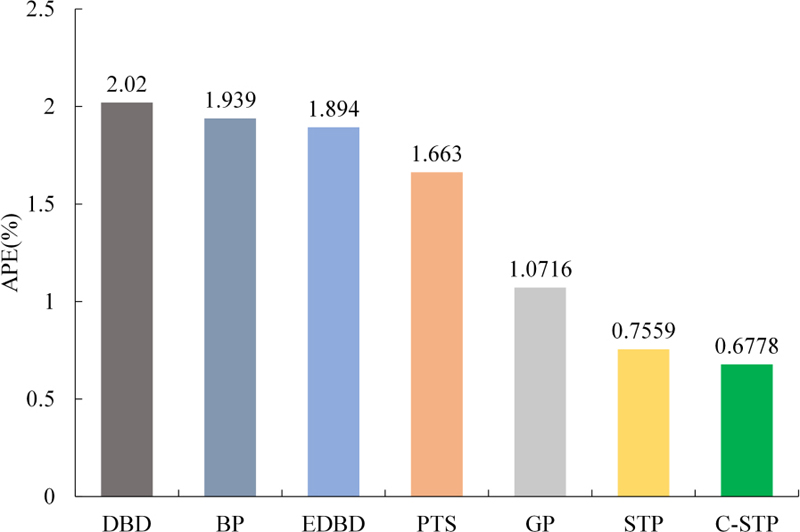
Figure 7: APE of different models for the RMSA.
As shown in Table 4 and Fig. 5, the prediction accuracy of the proposed C-STP is 84.96% higher than that of BP, 31.51% higher than that of SVM, 15.50% higher than that of GP, and 7.28% higher than that of STP. The APE of the proposed C-STP is only 1.5498%, showing its strong generalization performance and effectiveness.
In the following, the resonant frequency of RMSA [36, 37], shown in Fig. 6, is selected for testing the proposed C-STP. The antenna consists of a radiating element, a dielectric layer and a ground plane, and , , , represent the corresponding width, length, thickness of dielectric substrate and relative dielectric constant, respectively. A total of 33 groups of samples are shown in Table 5, which is divided into two parts, one as training set and the other as a test set. A total of 26 groups of samples are randomly selected as the training set, and the remaining 7 groups are marked with * symbol as the test set. The input are , , , , and the resonant frequency is used as the output. The evaluation metric for the experiment is still the APE.
Six modelling methods including Delta-bar-delta (DBD) [38], BP [38], Extended Delta-bar-delta (EDBD) [38], Parallel Tabu Search (PTS) [39], GP [34], and STP are selected as comparison. The test results are shown in Table 6 and Fig. 7. It can be seen that the predicted APE of the proposed C-STP is 0.6778% and less than that of the other six modelling methods, which is 10.33% higher than STP, 35.24% higher than GP, and 58.27% higher than PTS. It is 63.36% higher than the EDBD method, 64.2% higher than the BP method, and 65.64% higher than the DBD method. Therefore, the C-STP has excellent generalization performance forthe RMSA.
V. CONCLUSION
This paper proposes an algorithm named Consistent Student’s-T Process (C-STP), aiming to improve the accuracy and efficiency of antenna optimization by exploiting the consistent results of multiple STP instances and reducing the uncertainty of independently trained STP results. The core idea of the proposed C-STP is to process multiple independently trained STP results through a consistent algorithm to improve the possible inaccuracy problem when using only one STP. The experimental results show that the proposed C-STP algorithm has a clear advantage over existing algorithms in modelling and optimizing the resonant frequencies of two microstrip antennas in accuracy. In addition, the proposed algorithm can overcome the limitations of small sample data and achieve more reliable modelling and optimization results by consistent results from multiple STP instances. Similarly, the proposed method can also be easily applied to the modelling and optimization of other electromagnetic devices.
In practical applications, the optimization of antennas has to take into account the limited time and available computer resources. The proposed C-STP model uses imperfectly trained STPs for the optimization, as well as the estimation of output uncertainty through a consistency approach. We also find that the predictive ability of the model is strongly related to the choice of kernel function and individual network models, and we will continue to investigate in the following study. The proposed method is less suitable for higher dimensionality and larger data volume EM models, which require a large amount of time for training, resulting in low-cost performance.
ACKNOWLEDGMENT
This work was supported by the Natural Science Foundation of Guangdong Province of China under Grant No.2023A1515011272, the Tertiary Education Scientific research project of Guangzhou Municipal Education Bureau of China under No.202234598, the special project in key fields of Guangdong Universities of China under No.2022ZDZX1020, and the scientific research capacity improvement project of key developing disciplines in Guangdong Province of China under No.2021ZDJS057. Corresponding to Yubo Tian, Xuefeng Ren and Yubo Tian are co-first authors.
REFERENCES
[1] Z. Jiang, Y. Zheng, X. Xuan, and N. Nie, “A novel ultra-wideband wide-angle scanning sparse array antenna using genetic algorithm,” Applied Computational Electromagnetics Society (ACES) Journal, vol. 38, no. 2, pp. 100-108, 2023.
[2] V. Grout, M. O. Akinsolu, B. Liu, P. I. Lazaridis, K. K. Mistry, and Z. D. Zaharis, “Software solutions for antenna design exploration: A comparison of packages, tools, techniques, and algorithms for various design challenges,” IEEE Antennas and Propagation Magazine, vol. 61, no. 3, pp. 48-59, 2019.
[3] L.-Y. Xiao, W. Shao, F.-L. Jin, B.-Z. Wang, and Q. H. Liu, ‘‘Inverse artificial neural network for multiobjective antenna design,” IEEE Transactions on Antennas and Propagation, vol. 69, no. 10, pp. 6651-6659, 2021.
[4] L.-Y. Xiao, W. Shao, X. Ding, Q. H. Liu, and W. T. Joines, “Multigrade artificial neural network for the design of finite periodic arrays,” IEEE Transactions on Antennas and Propagation, vol. 67, no. 5, pp. 3109-3116, 2019.
[5] A. Uluslu, “Application of artificial neural network base enhanced MLP model for scattering parameter prediction of dual-band helical antenna,” Applied Computational Electromagnetics Society (ACES) Journal, vol. 38, no. 5, pp. 316-324, 2023.
[6] A. Ibrahim, H. Abutarboush, A. Mohamed, M. Fouad, and E. El-Kenawy, “An optimized ensemble model for prediction the bandwidth of metamaterial antenna,” CMC-Computers, Materials & Continua, vol. 71, no. 1, pp. 199-213, 2022.
[7] D. Shi, C. Lian, K. Cui, Y. Chen, and X. Liu, “An intelligent antenna synthesis method based on machine learning,” IEEE Transactions on Antennas and Propagation, vol. 70, no. 7, pp. 4965-4976, 2022.
[8] J. Nan, H. Xie, M. Gao, Y. Song, and W. Yang, “Design of UWB antenna based on improved deep belief network and extreme learning machine surrogate models,” IEEE Access, vol. 9, pp. 126541-126549, 2021.
[9] S. Han and Y. Tian, “Structure parameter estimation method for microwave device using dimension reduction network,” International Journal of Machine Learning and Cybernetics, vol. 14, no. 4, pp. 1285-1301, 2023.
[10] L.-Y. Xiao, W. Shao, S.-B. Shi, and Z.-B. Wang, “Extreme learning machine with a modified flower pollination algorithm for filter design,” Applied Computational Electromagnetics Society (ACES) Journal, vol. 33, no. 03, pp. 279-284, 2021.
[11] K. Sharma and G. P. Pandey, “Efficient modelling of compact microstrip antenna using machine learning,” AEU-International Journal of Electronics and Communications, vol. 135, p. 153739, 2021.
[12] X. Chen, Y. Tian, T. Zhang, and J. Gao, “Differential evolution based manifold Gaussian process machine learning for microwave Filter s parameter extraction,” IEEE Access, vol. 8, pp. 146450-146462, 2020.
[13] J. Gao, Y. Tian, X. Zheng, and X. Chen, “Resonant frequency modeling of microwave antennas using Gaussian process based on semisupervised learning,” Complexity, vol. 2020, p. 12, 2020.
[14] F. Pang, J. Ji, J. Ding, W. Zhang, D. Xu, and M. Zhou, “Analyze the crosstalk of multi-core twisted wires and the effect of non-matched impedance based on BSAS-BPNN algorithm,” Applied Computational Electromagnetics Society (ACES) Journal, vol. 38, no. 2, pp. 80-90,2023.
[15] S. Han, Y. Tian, W. Ding, and P. Li, “Resonant frequency modeling of microstrip antenna based on deep kernel learning,” IEEE Access, vol. 9, pp. 39067-39076, 2021.
[16] A. O’Hagan, “On outlier rejection phenomena in Bayes inference,” Journal of the Royal Statistical Society Series B: Statistical Methodology, vol. 41, no. 3, pp. 358-367, 1979.
[17] A. Shah, A. Wilson, and Z. Ghahramani, “Student-t processes as alternatives to Gaussian processes,” in Artificial Intelligence and Statistics, pp. 877-885, PMLR, 2014.
[18] A. Solin and S. Särkkä, “State space methods for efficient inference in Student-t process regression,” Artificial Intelligence and Statistics, vol. 38, pp. 885-893, PMLR, 2015.
[19] Q. Tang, L. Niu, Y. Wang, T. Dai, W. An, J. Cai, and S.-T. Xia, “Student-t process regression with student-t likelihood,” in IJCAI, pp. 2822-2828, 2017.
[20] Z. Chen, B. Wang, and A. N. Gorban, “Multivariate Gaussian and student-t process regression for multi-output prediction,” Neural Computing and Applications, vol. 32, pp. 3005-3028, 2020.
[21] R. B. Gramacy and H. K. H. Lee, “Bayesian treed Gaussian process models with an application to computer modeling,” Journal of the American Statistical Association, vol. 103, no. 483, pp. 1119-1130, 2008.
[22] C. E. Rasmussen, “Gaussian processes in machine learning,” Summer School on Machine Learning, pp. 63-71, Springer, 2003.
[23] B. D. Tracey and D. Wolpert, “Upgrading from Gaussian processes to student’s-t processes,” in 2018 AIAA Non-Deterministic Approaches Conference, p. 1659, 2018.
[24] J. Vanhatalo, P. Jylänki, and A. Vehtari, “Gaussian process regression with student-t likelihood,” Advances in Neural Information Processing Systems, vol. 22, 2009.
[25] Q. T. Y. Wang and S.-T. Xia, “Student-t process regression with dependent student-t noise,” in ECAI 2016: 22nd European Conference on Artificial Intelligence, vol. 29 of ECAI’16, pp. 82-89, IOS Press, NLD, 2016.
[26] R. K. Singh, A. Choudhury, M. Tiwari, and R. Shankar, “Improved Decision Neural Network (IDNN) based consensus method to solve a multi-objective group decision making problem,” Advanced Engineering Informatics, vol. 21, no. 3, pp. 335-348, 2007.
[27] D. Wu, K. Gong, K. Kim, X. Li, and Q. Li, “Consensus neural network for medical imaging denoising with only noisy training samples,” in International Conference on Medical Image Computing and Computer-Assisted Intervention, pp. 741-749, Springer-Verlag, 2019.
[28] Z. Ž. Stanković, D. I. Olćan, N. S. Dončov, and B. M. Kolundžija, “Consensus deep neural networks for antenna design and optimization,” IEEE Transactions on Antennas and Propagation, vol. 70, no. 7, pp. 5015-5023, 2021.
[29] T. Goel, R. T. Haftka, W. Shyy, and N. V. Queipo, “Ensemble of surrogates,” Structural and Multidisciplinary Optimization, vol. 33, pp. 199-216, 2007.
[30] C. L. Blake, “UCI repository of machine learning databases,” http://www.ics.uci.edu/~mlearn/MLRepository.html, 1998.
[31] C.-C. Chang and C.-J. Lin, “LIBSVM: A library for support vector machines,” ACM Transactions on Intelligent Systems and Technology (TIST), vol. 2, no. 3, pp. 1-27, 2011.
[32] J. S. Armstrong and F. Collopy, “Error measures for generalizing about forecasting methods: Empirical comparisons,” International Journal of Forecasting, vol. 8, no. 1, pp. 69-80, 1992.
[33] G.-B. Huang, Q.-Y. Zhu, and C.-K. Siew, “Extreme learning machine: a new learning scheme of feedforward neural networks,” in 2004 IEEE International Joint Conference on Neural Networks (IEEE Cat. No.04CH37541), vol. 2, pp. 985-990, 2004.
[34] M. Ebden, “Gaussian processes: A quick introduction,” arXiv preprint arXiv:1505.02965, 2015.
[35] Ş. Sağiroğlu, K. Güney, and M. Erler, “Resonant frequency calculation for circular microstrip antennas using artificial neural networks,” International Journal of RF and Microwave Computer-Aided Engineering, vol. 8, no. 3, pp. 270-277, 1998.
[36] M. Kara, “Closed-form expressions for the resonant frequency of rectangular microstrip antenna elements with thick substrates,” Microwave and Optical Technology Letters, vol. 12, no. 3, pp. 131-136, 1996.
[37] M. Kara, “The resonant frequency of rectangular microstrip antenna elements with various substrate thicknesses,” Microwave and Optical Technology Letters, vol. 11, no. 2, pp. 55-59, 1996.
[38] K. Guney, S. Sagiroglu, and M. Erler, “Generalized neural method to determine resonant frequencies of various microstrip antennas,” International Journal of RF and Microwave Computer-Aided Engineering, vol. 12, no. 1, pp. 131-139, 2002.
[39] S. Sagiroglu and A. Kalinli, “Determining resonant frequencies of various microstrip antennas within a single neural model trained using parallel tabu search algorithm,” Electromagnetics, vol. 25, no. 6, pp. 551-565, 2005.
BIOGRAPHIES

Xuefeng Ren studying in JiangsuUniversity of science and technology, master’s degree, research direction: intelligent optimization algorithm,intelligent electromagnetic optimi-zation.

Yubo Tian was born in Tieling, Liaoning Province, China, in 1971. He received the Ph.D. degree in radio physics from the Department of Electronic Science and Engineering, Nanjing University, Nanjing, China. From 1997 to 2004, he was with the Department of Information Engineering, Shenyang University, Shenyang, China. From 2005 to 2020, he was with the School of Electronics and Information, Jiangsu University of Science and Technology, Zhenjiang, China. He is currently with the School of Information and Communication Engineering, Guangzhou Maritime University, Guangzhou, China. His current research interest is Machine Learning methods and their applications in electronics and electromagnetics.

Qing Li was Born in Anqing, Anhui Province, China, studying in Jiangsu University of science and technology, master’s degree, research direction: intelligent optimization algorithm, intelligent electromagnetic optimization.

Hao Fu studying in Jiangsu University of science and technology,master’s degree, research direction: intelligent optimization algorithm,intelligent electromagnetic optimi-zation.
ACES JOURNAL, Vol. 38, No. 12, 987–997
doi: 10.13052/2023.ACES.J.381209
© 2023 River Publishers