Electromagnetic Scattering from a Three-dimensional Object using Physics-informed Neural Network
Yuan Zhang, Renxian Li, Huan Tang, Zhuoyuan Shi, Bing Wei, Shuhong Gong, Lixia Yang, and Bing Yan
1School of Physics, Xidian University
Xi’an 710071, China
zhangyuan9938@163.com, rxli@mail.xidian.edu.cn, 1327441185@qq.com,
zhuoyuans2000@163.com, bwei@xidian.edu.cn, shgong@xidian.edu.cn
2Information Materials and Intelligent Sensing Laboratory of Anhui Province
Anhui University, China
lixiayang@yeah.net
3School of Information and Communication Engineering
North University of China 030051, China
yanbing122530@126.com
4Shanxi Key Laboratory of Signal Capturing and Processing
North University of China, 030051, Shanxi Taiyuan, China
yanbing122530@126.com
Submitted On: July 20, 2023; Accepted On: January 9, 2024
ABSTRACT
Prediction of electromagnetic fields scattered from objects is of great significance in various fields. Traditional computational electromagnetic solvers, which are mesh-based, are expensive and time-consuming. The deep learning technique becomes an alternative method of the prediction of scattered fields with high efficiency. However, the data-driven deep learning method requires a large data set and lacks robustness. For complicated scattering problems, the construction of a large training data set is a hard task. By considering physics-constraints, physics-informed neural networks (PINNs) can solve the partial differential equation (PDE) problem with a small data set and also provide a physical explanation. In this paper, the PINNs are employed to solve the scattering of a plane wave by a three-dimensional object with Maxwell’s equations being physical constraints. In the calculation, a sphere and an ellipsoid are taken as examples, and the effects of the network parameters (including the number of hidden layers, and the number of data sets) are mainly discussed. The results have practical applications in many fields such as radar detection, biomedical imaging, and satellite navigation.
Index Terms: electromagnetic scattering, Maxwell’s equations, physics-informed neural network.
I. INTRODUCTION
Many practical applications in medicine, aerospace, communication, and remote sensing [1, 2, 3, 4] involve the electromagnetic scattering by objects. The electromagnetic scattering problem refers to the study of the electromagnetic response resulting from the incident electromagnetic waves given the target and environmental information. Numerical methods can accurately predict the scattered field distribution of an isolated object. In the past developments, computational electromagnetics have provided the basis for solving many practical problems without analytic counterparts, and have become a popular mainstream approach for a wide range of researchers. However, traditional computational electromagnetic solvers such as the finite difference time domain (FDTD) [5, 6], the finite-element method (FEM) [7], and the finite difference frequency domain (FDFD) [8] are based on dividing the solution domain into a network of differences, and replacing the continuous solution domain with a finite number of mesh nodes. This method requires discretization and is solved by meshing the problem area. However, in many practical problems, the region is often not a regular and easy-to-fractionalise geometric region, and it is difficult to generate a mesh. Thus mesh-based methods cannot achieve good results and are very time-consuming and computationally expensive [9].
Meanwhile, as artificial intelligence (AI) technology explodes, researchers are trying to apply neural networks to computational electromagnetics as a replacement method for predicting scattered fields. Deep learning (DL) methods such as convolutional neural networks (CNN), recurrent neural networks (RNN), and generative adversarial networks (GANs) have led to amazing advances in the field of computational physics in modeling physical learning agents [10]. Deep learning techniques can identify the hidden rules of the ’action-reaction’ behavior of the control system through a certain learning process [11], which is based on the principle of establishing a functional mapping between the input data and the output data. The optimization capabilities and coded boundary conditions of deep learning can improve the accuracy and efficiency of electromagnetic simulations by capturing complex behaviors, providing implicit representations, enabling generalization, reducing computational costs, and enabling efficient parallelization. Deep learning models are capable of capturing the intricate nonlinear relationships in data. By encoding boundary conditions that are critical in electromagnetic simulations, models can learn complex behaviors and interactions at the boundary more efficiently than traditional interpolation techniques. This allows for a more accurate representation of electromagnetic fields and their propagation. At the same time, the deep learning model can generalize from limited training data to unknown scenarios. Once trained on a different set of boundary conditions, the model can accurately predict the electromagnetic field for new boundary conditions outside the training dataset. This generalization capability greatly improves the accuracy of the simulation, especially when it is impractical or costly to obtain a large number of training samples. In contrast, traditional function interpolation techniques typically require a dense grid of points to accurately represent the electromagnetic field, which can lead to costly simulation calculations. Various studies have shown that machine-learning-based algorithms have promising applications in the field of solving partial differential equations [5], which can largely reduce the memory required for computation and are simple and easy to implement and can well meet the needs of electromagnetic properties for engineering applications. Traditional deep learning methods are purely data-driven and require large datasets for training. However, for some complex scatterers, large training data sets are not available. Also, in many physics and engineering fields, these training data often imply partial a priori knowledge (e.g., electric field data satisfying the Maxwell system of equations), but the pure data drive ignores this partial knowledge.
The limitations of the above methods have largely contributed to the emergence of physics-informed neural networks (PINNs). Lagaris et al. [12] pioneered the similarity between neural network training and solving partial differential equations, and neural networks of physics knowledge were proposed for solving Maxwell’s set of equations for scattering problems. In this case, the network constructs a mapping of spatial and temporal coordinates to the corresponding electromagnetic field at that point. At the same time, the gradient of the electric field concerning the spatial coordinates can be calculated quickly by using the automatic differentiation algorithm, which speeds up the numerical calculation of the partial differential equation. Compared with the standard numerical methods in traditional computational electromagnetics, the computational efficiency is significantly improved. In 2019, Raissi [13] classifies the model equation as a physical driver as a regularization term and encodes it into the neural network by adding the loss of the control equation and the loss of the boundary conditions and initial conditions to the loss function. Under the condition of the small dataset, we successfully learned a model with stronger generalization ability. It not only learns the distribution law of training data samples like traditional neural networks, but also learns the physical laws described by mathematical equations, and can learn more generalized models with fewer data samples, which solves the difficulties of decision-making and prediction caused by the unavailability of traditional deep neural networks and the scarcity of data. In summary, the PINNs have great advantages in the field of computational electromagnetics, and the development prospects are very promising in saving memory, improving prediction accuracy, and solving high-dimensional complex problems.
In this contribution, we build a fully connected neural network, encode physical information such as Maxwell’s equations and boundary conditions as constraints into the neural network, and study the electromagnetic scattering from a three-dimensional object by training the built network model with a sphere and an ellipsoid as examples. We compare the prediction results based on the PINNs method with the analytical solution by Mie theory (for sphere ) or numerical results by FDFD (for ellipsoid) to verify the feasibility and accuracy of our work, and the effects of network parameters are mainly discussed. The full paper is divided into four parts, and in the second part, we introduce our proposed PINNs. In the third part, we give the simulation results of PINNs and discuss the effects of network structure and hyperparameters on the results. The fourth part is a summary of the paper.
II. METHODOLOGY AND FORMULATION
A. Deep learning framework
In this paper, we propose a deep learning method for solving Maxwell’s equations, using the powerful optimization capability of deep learning to solve the frequency-domain electromagnetic field. In this approach, we encode the boundary conditions (BC), and Maxwell’s equations as regularization terms of the network so that it approximates the analytic solution infinitely. According to the electromagnetism uniqueness theorem [14], Maxwell’s equations can be solved uniquely for known boundary conditions. Thus, we successfully transformed an electromagnetic forward modeling problem into an optimization process.
B. Details and implementation
Assuming a time dependence , the scattered magnetic field satisfies the following vector wave equation:
| (1) |
where, is the angular frequency, is the magnetic permeability, is the electric permittivity, and and are the magnetic permeability and electric permittivity of a vacuum, respectively. and are the scattered and incidence magnetic fields, respectively.
Next, we will use the PINNs to solve the vector wave equation (1). Figure 1 shows a schematic of the neural network layout. We first define a network with parameters to represent the surrogate of the equation solution.
Due to the frequency domain approach, in the PINNs model shown in Fig. 1, the input to the network is the spatial coordinates of the solution area without temporal information, and the output is the real and imaginary parts of the scattered magnetic field, which is denoted by in Fig. 1.
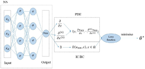
Figure 1: Representative diagram of the physics-informed neural network model.
Therefore, the loss function can be divided into three parts, which are , , and :
| (2) |
where:
| (3) |
and corresponds to the data constraints. and denote the predicted and true values, respectively. corresponds to the boundary condition. Note that, in our model, we only consider the boundary conditions at the outer boundary of the perfectly matched layer (PML), where the scattered magnetic fields vanish and . enforces the vector wave equations at a certain set of points. Unlike traditional deep learning, this loss function considers physical information constraints. , , and denote the residual points for , , and , respectively.
In this paper, we use Mean Absolute Error (MAE) to assess model performance. MAE is a common metric used in regression problems to assess the performance of predictive models. It measures the average absolute difference between the predicted and actual values in the data set. The MAE does not cancel out positively or negatively because the deviation is absolutised, thus, the mean absolute error better reflects the actual situation of the prediction value error.
To define the functions , , and in equation (3), the object is assumed to be surrounded by a PML to prevent the wave from reflecting from the boundary and re-entering the simulation domain.
In this paper we use the stretched-coordinate PML (SC-PML), and , , and can be defined as:
| (4) |
where , , and are parameters to define PML. The partial derivative of equation (4) can be obtained using automatic differentiation, which can be achieved by using the function torch.autograd.grad.
Then the network is trained to find the best parameters () by minimizing the total loss defined by equation (2) via gradient optimizers, such as Adam and L-BFGS, until the loss is smaller than athreshold .
In our simulation, a fully connected neural network is selected, the input of the network is spatial coordinates, and the output is the real and imaginary parts of the magnetic field, i.e., in the case of a sphere, the network input is three-dimensional () and the output is six-dimensional ( and with ). The network has many hidden layers and each hidden layer contains several neurons. Meanwhile, we use the L-BFGS algorithm for optimization, and the spatial coordinate points of each random sampling point are generated by Latin hypercube sampling, which is a very practical sampling method that can be achieved by calling function pyDOE, lhs.
III. NUMERICAL RESULTS AND DISCUSSION
In this section, we use the neural network given in Section II. to simulate electromagnetic scattering by three-dimensional objects. After the neural network is first verified by the comparison of its results with the analytical results calculated by Mie theory by taking a sphere as the example of an object, the effects of the number of labeled data and network structure are mainly discussed.
Next, the method is used for the electromagnetic scattering by an ellipsoid.
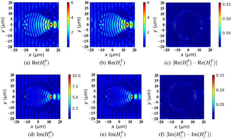
Figure 2: Simulation results of the electromagnetic field in xoy plane.
A. Validation
To validate the feasibility of our proposed network, we choose a three-dimensional homogeneous sphere as an example to study the electromagneticresponse.
In the calculation, the radius and the refractive index of the particle are with being the wavelength and , respectively.
The incident wave is a transverse magnetic (TM) polarized plane wave propagating along the -axis, and its wavelength is . We set , , and . The spatial coordinates of all randomly sampled points are generated using Latin hypercube sampling.
All labeled data are calculated using Mie theory. We use a fully connected neural network, which contains four hidden layers and has neurons per layer. In simulation, we take the ratio of training set and test set as 9:1.
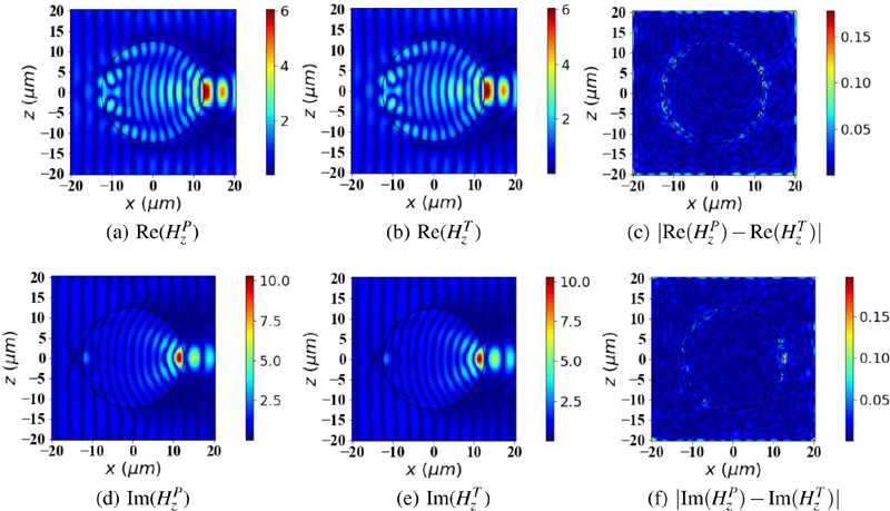
Figure 3: Simulation results of the electromagnetic field in xoz plane.
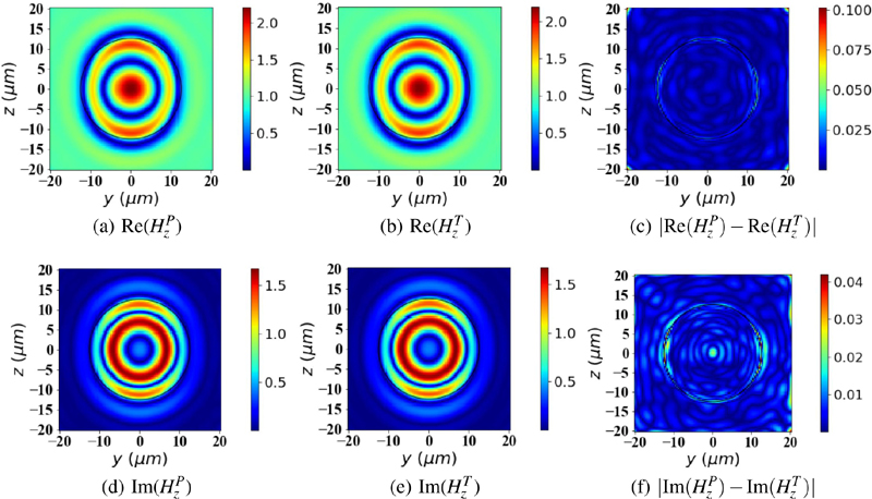
Figure 4: Simulation results of the electromagnetic field in yoz plane.
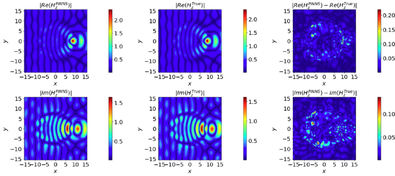
Figure 5: Simulation results for the xoy plane electromagnetic field of an ellipsoid.
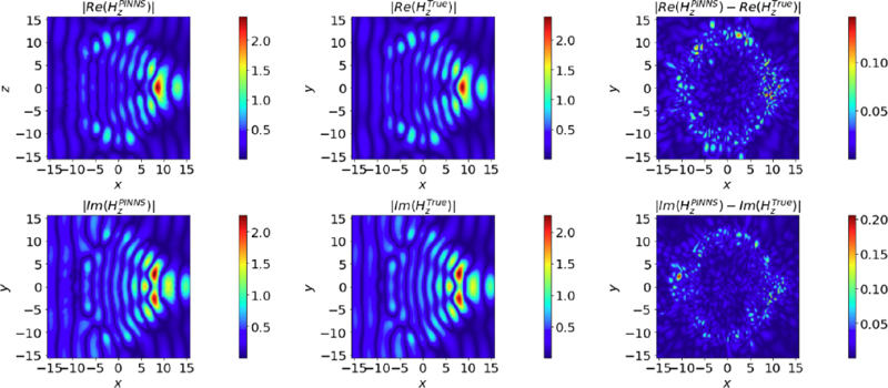
Figure 6: Simulation results for the xoz plane electromagnetic field of an ellipsoid.
Figures 2–4 give the simulated magnetic fields in , , and planes, respectively.
In each figure, the black circle indicates the object boundary.
Each figure includes six sub-figures, which are divided into two rows and three columns. The upper row gives the real part of , and the lower row is the imaginary part. The left column gives the results predicted by PINNs (denoted by superscript ), the middle column gives the ground true results by the Mie theory (denoted by superscript ), and the right column gives theerrors.
It can be observed from the first and second columns of Fig. 2 that in the plane the results predicted by the PINNs are in good agreement with the ground true values. From the right column of Fig. 2, we can see that the maximum absolute errors for the real and imaginary parts of are respectively about and , which correspond to the maximum relative errors about and . This indicates that the prediction accuracy of the network structure we built is high enough to achieve the results we expected. From (Fig. 3) and (Fig. 4), we can also find the high accuracy of the PINNs.
It can be seen from the third column of Fig. 3 that the maximum absolute errors of the real and imaginary parts of in the plane are about and , which correspond to the maximum relative errors and . Similar analysis shows that in the plane the maximum absolute errors of the real and imaginary parts of are about and , which correspond to the maximum relative errors and .
B. Effect of labeled data
Theoretically, increasing the number of labeled data can lead to a more improved approximation of the neural network during training. Therefore, we investigate the effect of different amounts of labeled data on the prediction results by PINNs. In the calculation, all other conditions are consistent, and the number of labeled data varies. All the labeled data are calculated using Mietheory.
Table 1 gives the average absolute errors of results by PINNs with respect to that by Mie theory. The table has three columns. The first column is the number of labeled data. The second and third columns give the errors of the real and imaginary parts of , respectively. From Table 1, we can see that the prediction accuracy gradually increases as the number of labeled data increases. This says that by adding labeled data we can obtain predicted results with higher accuracy. A reminder that in our calculation, the object is a sphere and the ground true results can be easily obtained using Mie theory. However, if the object is very complicated, it is hard to obtain a large number of labeleddata.
Table 1: Average absolute error versus labeled datanumber
| Data | ||
C. Effect of network architecture
We also need to investigate the effect of parameter settings and the structure of neural networks on prediction accuracy. We vary the number of hidden layers () and the number of neurons per layer () to observe the change in prediction accuracy and evaluate the network training effect while keeping other parameters constant. The average absolute errors of are shown in Table 2. The table has four columns and four rows. The first column gives the number of hidden layers , and the second to fourth columns gives the errors for various number of neurons . The first row gives the number of neurons , and the second to fourth rows gives the errors for various number of hidden layers . Note that all cells except the first row and column have two numbers. The upper number is the error of the real part of , and the lower number is that for the imaginary part. As we expected, the network prediction accuracy improves as the number of layers and neuronsincreases.
Table 2: Average absolute error versus number of hidden layers () and neurons in each layer ()
| 3 Layers | |||
| 4 Layers | |||
| 5 Layers | |||
D. Further expansion
To explore the applicability of the proposed network in different scenarios, we also briefly investigate the electromagnetic response of 3D ellipsoidal particles. In the calculations, the major axis and minor axis of the ellipsoidal particles are and , respectively, and all other parameters are the same as those of the spherical particles.
The simulated magnetic fields in the and planes are given in Figs. 5 and 6, respectively. Unlike the plot for the sphere, the middle column shows the true result derived by the FDFD (denoted by superscript ).
It can be seen that the predicted values of PINNs are in better agreement with the true values in the and planes.
From the right column of Fig. 5, we can see that the maximum absolute errors for the real and imaginary parts of are respectively about and , which correspond to maximum relative errors of about in both cases.
From (Fig. 6), we can see that the maximum absolute errors for the real and imaginary parts of are respectively about and , which correspond to the maximum relative errors about and .
The errors are concentrated at the edge positions of the ellipsoid, which we analyse to be due to the discontinuity of the dielectric constant at the edge positions. The PINN predictions match the true values at all positions except the edge position.
This shows that the prediction accuracy of our constructed network structure can reach our expected results.
IV. CONCLUSION
The electromagnetic scattering by a three-dimensional target is investigated using physics-informed neural networks (PINNs). Under the physical constraint of Maxwell’s equations, the total magnetic fields of a TM plane wave scattering by a homogeneous sphere is predicted with high accuracy. The effects of the number of labeled data, and network structures on the prediction results are mainly discussed.
ACKNOWLEDGMENT
The authors acknowledge the support from the National Natural Science Foundation of China [62001345, 61901324, 61771375, 92052106], the open fund of Information Materials and Intelligent Sensing Laboratory of Anhui Province [IMIS202103], and the Project of Natural Science Research in Shanxi Province[202203021211095].
REFERENCES
[1] M. S. Zhdanov, Geophysical Inverse Theory and Regularization Problems, vol. 36, Amsterdam: Elsevier, 2002.
[2] A. Abubakar, P. M. Van den Berg, and J. J. Mallorqui, “Imaging of biomedical data using a multiplicative regularized contrast source inversion method,” IEEE Transactions on Microwave Theory and Techniques, vol. 50, no. 7, pp. 1761-1771, 2002.
[3] X. Wang, T. Qin, R. S. Witte, and H. Xin, “Computational feasibility study of contrast-enhanced thermoacoustic imaging for breast cancer detection using realistic numerical breast phantoms,” IEEE Transactions on Microwave Theory and Techniques, vol. 63, no. 5, pp. 1489-1501, 2015.
[4] C. A. Balanis, Antenna Theory: Analysis and Design, New York: Wiley, 2016.
[5] A. Taflove, S. C. Hagness, and M. Piket-May, “Computational electromagnetics: The finite-difference time-domain method,” The Electrical Engineering Handbook, vol. 3, pp. 629-670,2005.
[6] K. Yee, “Numerical solution of initial boundary value problems involving Maxwell’s equations in isotropic media,” IEEE Transactions on Antennas and Propagation, vol. 14, no. 3, pp. 302-307,1966.
[7] J.-M. Jin, The Finite Element Method in Electromagnetics, New York: Wiley, 2015.
[8] R. C. Rumpf, “Simple implementation of arbitrarily shaped total-field/scattered-field regions in finite-difference frequency-domain,” Progress In Electromagnetics Research B, vol. 36, pp. 221-248, 2012.
[9] J. Smajic, C. Hafner, L. Raguin, K. Tavzarashvili, and M. Mishrikey, “Comparison of numerical methods for the analysis of plasmonic structures,” Journal of Computational and Theoretical Nanoscience, vol. 6, no. 3, pp. 763-774, 2009.
[10] A. Massa, D. Marcantonio, X. Chen, M. Li, and M. Salucci, “DNNs as applied to electromagnetics, antennas, and propagation—A review,” IEEE Antennas and Wireless Propagation Letters, vol. 18, no. 11, pp. 2225-2229, 2019.
[11] Y. Li, Y. Wang, S. Qi, Q. Ren, L. Kang, S. D. Campbell, P. L. Werner, and D. H. Werner, “Predicting scattering from complex nano-structures via deep learning,” IEEE Access, vol. 8, pp. 139983-139993, 2020.
[12] I. E. Lagaris, A. Likas, and D. I. Fotiadis, “Artificial neural networks for solving ordinary an partial differential equations,” IEEE Transactions on Neural Networks, vol. 9, no. 5, pp. 987-1000, 1998.
[13] M. Raissi, P. Perdikaris, and G. E. Karniadakis, “Physics-informed neural networks: A deep learning framework for solving forward and inverse problems involving nonlinear partial differential equations,” Journal of Computational Physics, vol. 378, pp. 686-707, 2019.
[14] L. D. Landau, The Classical Theory of Fields, vol. 2, Amsterdam: Elsevier, 2013.
BIOGRAPHIES

Yuan Zhang received the B.S. degree from Xidian University, Xi’an, China, in 2021. She is currently working toward the M.S. degree in Optics, Xidian University. Her research interests include machine learning, and computational electromagnetism.

Renxian Li received the Ph.D. degree from Xidian University in 2008. After graduation, he joined the School of Physics, Xidian University. His research interests includes machine learning, electromagnetic scattering, and computational electromagnetism.

Huan Tang received the B.S. degree from Xidian University, Xi’an, China, in 2020. He is currently working toward the Ph.D. degree in Optics, Xidian University. His research interests include neural network, and electromagnetic scattering.

Zhuoyuan Shi received the B.S. degree from Xidian University, Xi’an, China, in 2022. She is currently working toward the M.S. degree in Optics, Xidian University. Her research interests include machine learning, and electromagnetic scattering.

Bing Wei was born in July 1970, graduated from Beijing Normal University in 1993, majoring in Solid State and Ion Beam Physics, and received his Ph.D. degree in Radio Physics from Xidian University of Electronic Science and Technology (XUET) in 2004. He is now a professor of Xidian University of Electronic Science and Technology (XUET), a doctoral supervisor of radio

Shuhong Gonggong was born in Shanxi, China, in 1978. He received the B.S. degree in physics education from Shanxi Normal University, Xi’an, China, in 2001, the M.S. and Ph.D. degrees in radio physics from Xidian University, Xi’an, in 2004 and 2008, respectively. He is currently a Professor at Xidian University. His research work has been focused on novel antenna design, radio wave propagation, and their applications.

Lixia Yangyang was born in Ezhou, Hubei, China, in 1975. He received the B.S. degree in physics from Hubei University, Wuhan, China, in 1997, and the Ph.D. degree in radio physics from Xidian University, Xi’an, China, in 2007.
Since 2010, he has been an Associate Professor with the Communication Engineering Department, Jiangsu University, Zhenjiang, China. From 2010 to 2011, he was a Postdoctoral Research Fellow with the Electro Science Laboratory (ESL), The Ohio State University, Columbus, OH, USA. From 2015 to 2016, he was a Visiting Scholar with the Institute of Space Science, The University of Texas at Dallas, Dallas, TX, USA. From 2016 to 2019, he has been a Professor, a Ph.D. Supervisor, and the Chairman of the Communication Engineering Department, Jiangsu University. Since 2020, he has been a Distinguished Professor, a Ph.D. Supervisor, and the Vice Dean with the School of Electronic and Information Engineering, Anhui University, Hefei, China. His research interests include wireless communication technique, radio sciences, the computational electromagnetic, and the antenna theory and design in wireless communication systems. He is a member of the Editor Board of Radio Science Journal in China.

Bing Yanyan was born on October 6, 1976. From 2004 to 2009, he studied in the School of Science, Xidian University, and received his doctorate. In recent years, his interesting has been engaged in the research of gas-solid two-phase flow multi-parameter measurement based on light scattering method and electrostatic method.
ACES JOURNAL, Vol. 40, No. 2, 103–111
doi: 10.13052/2025.ACES.J.400203
© 2025 River Publishers