Physics-informed Neural Networks for the Resolution of Analysis Problems in Electromagnetics
S. Barmada, P. Di Barba, A. Formisano, M. E. Mognaschi, and M. Tucci
1DESTEC, University of Pisa, Pisa, Italy
sami.barmada@unipi.it, mauro.tucci@unipi.it
2Dept. of Electrical, Computer and Biomedical Engineering, University of Pavia, Pavia, Italy
paolo.dibarba@unipv.it, eve.mognaschi@unipv.it
3Dept. of Engineering, University of Campania “Luigi Vanvitelli,” Aversa, Italy
alessandro.formisano@unicampania.it
Submitted On: July 26, 2023; Accepted On: December 12, 2023
ABSTRACT
Learning from examples is the golden rule in the construction of behavioral models using neural networks (NN). When NN are trained to simulate physical equations, the tight enforcement of such laws is not guaranteed by the training process. In addition, there can be situations in which providing enough examples for a reliable training can be difficult, if not impossible. To alleviate these drawbacks of NN, recently a class of NN incorporating physical behavior has been proposed. Such NN are called “physics-informed neural networks” (PINN). In this contribution, their application to direct electromagnetic (EM) problems will be presented, and a formulation able to minimize an integral error will be introduced.
Keywords: Direct and inverse electromagnetic problems, neural networks, physics informed neural networks.
I. INTRODUCTION
Machine learning or neural network (NN) approaches are frequently adopted to create models of physical relationships, starting from a set of input-output examples: we can refer, for instance, to the computation of the magnetic field created by known sources in a set of measurement points (e.g., currents in assigned coils); this is usually referred to as forward problem. Data-driven approaches are applicable also for solving inverse problems (loosely speaking, recovering the source originating the observed field) [1–3], although their nature, usually ill-posed or ill-conditioned, requires dedicated countermeasures. As a matter of fact, data-driven approaches usually converge, under suitable but quite relaxed hypotheses, to some solution tightly related to the selection of examples and of the training paradigm. On the other hand, in the case of NN mimicking the behavior of physical systems, it is expected not only that the model is able to generalize its response to cases not included in the learning dataset but also that the underlying equations are fully respected. A second relevant issue related to the use of NN to simulate physical phenomena is the difficulty in creating datasets populated enough to grant reliable training. This is particularly relevant in cases where the data must be gathered from experiments, or from demanding simulations.
Recently, the concept of “physics-informed” learning started to be considered as a powerful aid to the construction of data-driven models converging to solutions with known properties [3]. The underlying concept is to try using the governing equations of the physical system as a priori knowledge, able to regularize the learning process, driving it towards acceptable solutions. Such a priori knowledge also helps in reducing the need for large datasets for the learning and testing of NN.
As a matter of fact, in several areas of physics including EM, physics-informed neural networks (PINNs) [4], with their compelling ability of learning solutions of partial differential equations (PDEs) without the need for providing examples, have gained popularity. However, first contributions to the use of neural networks for EM field analyses date back to the beginning of the 2000s. For instance, in [5] a finite element neural network (FENN) that embeds finite element models into a neural network format for solving Poisson’s equation was proposed. More recently, other relevant works [6, 7] dealing with electrostatic problems, made use of convolutional neural networks (CNNs). In particular, [6] highlighted the flexibility of CNNs in the case of complex distributions of excitation sources and dielectric constants. Since the introduction of PINNs, most applications in EM have involved optics [8–12]; more specifically, in [8] Maxwell’s equations were solved in the frequency domain with several model simplifications. The architecture was similar to the one of a generative adversarial network (GAN): the first part is reminiscent of a generator since it maps the space distribution of permittivity to the electric field distribution. The second part, i.e., the discriminator, evaluates how physically sound the generator’s outputs are. This enables, after training, the creation of a real-time field solver. This idea was re-introduced in [9] and put in a more general framework. In turn, [12] predicted the time evolution field in transient electrodynamics making use of an encoder-recurrent-decoder architecture. PINNs have also been used in magnetostatics and magneto-quasi-statics [13–16].
It can be noted that in most works (e.g., [2, 4, 10–14]), PINNs do not take system parameters (i.e., geometries, field sources, material properties) as an input and therefore they must be retrained, eventually taking advantage of transfer learning whenever the system parameters in the model must be changed. However, a few exceptions are reported in [8], [9], [15] where, once trained, PINNs could provide the solution of a class of direct field problems. This has been achieved by convolutional layers adopted in a GAN-like framework as in [8, 9]. More recently PINNs using dense layers and taking system parameters as input have been introduced [15], while in [16] an energy-based error function was used for training a PINN for the solution of magnetostatic problems.
Summing up, three mainstream methods could be categorized:
Data-driven networks: Starting from the available observations, this approach generates a (nonlinear) model not only able to reproduce the observed data but also to generalize on data not included in training datasets [17]. As an example, [18] proposes a PDE-Net to identify the governing PDE models by data learning, able to approximate the unknown nonlinear responses.
Physics-constrained networks: Within this further approach, physics constraints are introduced to strengthen the prediction ability of the NN, especially in the small data regime. Following the seminal paper [4], in [19] a physics-informed extreme learning machine (PIELM) to solve PDEs in complex domains was presented.
Algorithm optimization based on NN: More recently, the NN approach has been used to optimize the performance of classical numerical methods. In [20], for instance, a NN has been utilized for accelerating the numerical resolution of PDEs; this way, a substantial gain in computational efficiency over standard numerical methods was achieved.
In this contribution, a brief description of possible schemes to introduce partial differential equations in the structure of NN is first presented; this basically transforms a NN into a PINN, capable of self learning and not needing any pre-calculated training set. Then a simple electromagnetic problem is presented to show the effectiveness of PINN in the resolution of (direct) EM field problems. Finally, a perspective on PINN based on integral rather than pointwise error functional is presented.
II. PHYSICS INFORMED NEURAL NETWORKS
A. Local residual approach
To clarify ideas, let us consider a simple non-dynamical problem in EM field computation, described by Poisson equation, with suitable boundary conditions:
| (1) |
In (1), the time t is a simple parameter, but the PINN approach is general enough to treat also dynamical cases. represents the Laplacian of the unknown (scalar) function , is the spatial definition domain, and are the Dirichlet and Neumann parts of the boundary, respectively.
A NN model of (1) receives as input the coordinates of a point within and yields as output the value of the approximated solution , where represents the vector of weights and biases describing the NN. A possible approach to consider the a priori information about (1) is to define a representation error E, including a term related to the “residual” of the equation, and a second term related to boundary conditions:
| (2) |
where
| (3) |
and
| (4) |
where and are the assigned conditions on the Dirichlet and Neumann parts of the boundary, respectively, while represents the array of sampling points coordinate where error is evaluated we note that the term can be computed using the automated differentiation (AD) approach described in [4, 21]. When eq.(4) is evaluated using a norm, it is often referred to as energy-like error.
Figure 1 shows a general view of the training process of a PINN inspired by (1)-(4).
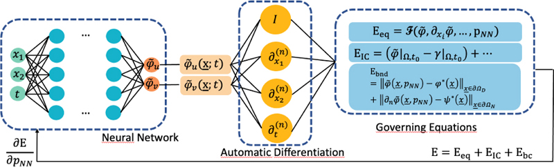
Figure 1: General architecture of a PINN for solving a PDE. E represents the error due to initial conditions in the case of dynamical problems, for the sake of simplicity.
B. Integral error approach
PINNs solving problems similar to (1) are usually trained based on the local residual of the governing equations [1, 2], and derivatives are typically evaluated by means of AD. Unfortunately, this approach could suffer from poor regularity. Domain decomposition represents a potential workaround [2], but only up to a certain degree. In this contribution, the authors propose an additional strategy, based on the minimization of an integral error instead of local quantities, much like the Rayleigh-Ritz method [22].
We start from the weighted residual form of (1):
| (5) |
where k is the material constant (permeability in the case of magnetostatics and permittivity in the case of electrostatics), and is a suitable Sobolev space, defined according to the boundary conditions. The solution will be defined in , the space of functions with correct boundary values on (which will be explicitly enforced at training time). Using standard calculus, eq.(5) can be reformulated as [22]:
| (6) |
Equation (6) can be discretized following a Galerkin approach, in which the weighting functions are selected as coincident with the elements of the representation basis for the unknown function. More in detail the approximate solution is defined as
| (7) |
where are the coefficients of the expansion, usually named nodal potentials in FEM-like expressions, is the weighting function, and is the number of output neurons. With this in mind, equations (6) and (7) lead to the following discretization.
| (8) |
Note that for the sake of simplicity in (8) we have highlighted just the dependence on output layer weights, but the argument of the functions does contain all the weights (and activation functions) of the hidden and input layers.
It is now necessary to turn (8) into an error function for the PINN training, with the aim of obtaining, at the end of the training step, a network able to provide a reliable approximation also for points not included in the training data. In view of this, a possible approach inspired by the Ritz formulation is to generate a training dataset from points in (and as well as on the boundaries and ) and compute integrals as discrete summations. Accordingly, the left-hand side term in (8) modifies as
| (9) |
We note that this approach corresponds to looking for the stationary points of the energy functional already defined in (4), the only difference, in this straightforward formulation, being that the training takes place only when all points have been processed (batch learning).
III. TEST CASES
A. Overall description
In this section, two test cases are shown. The first one presents the solution of a Poisson equation in a 1D domain. This simple problem serves as first validation relative to the use of PINNs for the solution of partial differential equations. It must be highlighted that in this implementation, the PINN does not need a training data-set: starting from a random guess solution, obtained by a random initialization of weights and biases, in a set of internal points (and on the boundary), the PINN evaluates the approximate solution , and at each epoch the physics-based error function (4) leads to an adjustment of the weights/biases. After the training is over, the PINN is capable of evaluating the function in points not necessarily coincident with the original set. This process can be referred to as self-training because no input-output pattern is externally supplied furthermore the possibility of freely selecting the evaluation points makes the PINN similar to a meshless method. In the following sections, the word “grid” is used to indicate the set of points . It is implicit that with this process a PINN trains itself on a specific set of points (grid) for this reason a change in the geometry necessarily leads to a new PINN, as it is for a new model in standard numerical methods.
A more complex 2D problem is then considered: this second example shows the accuracy of the method and its potential for the solution of general problems in presence of Neumann/Dirichlet boundary conditions. This problem is solved using the local residual approach in addition, the quantities object of the integral error approach are also shown together with a perspective overview.
B. 1D problem
To show the performance of the PINN approach to electromagnetic analysis, we first considered a simple one-dimensional problem ruled by the Poisson’s equation subject to Dirichlet boundary conditions. In particular, the problem to be solved is defined in and described in equation (769)
| (10) |
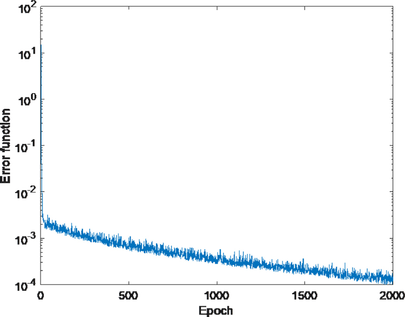
Figure 2: Error function history during training (1D problem).
Following the methodological approach (1)-(4), a shallow NN composed of one input layer fed with sampling point coordinates, and one hidden layer with 4 neurons, was synthesized. Sigmoidal functions were selected as the activation function stochastic gradient descent was the minimization algorithm, with random initialization of weights and biases and learning rate 510. sampling points were considered to compute E on the grid discretizing the domain in particular, the use of sigmoidal activation functions made it possible to analytically evaluate the second-order derivative in the Laplace operator. In Fig. 2 the training history of the network is shown in terms of error function against epochs, while in Fig. 3 the solution predicted by the trained PINN is represented.
After several experiments, an excellent agreement between predicted solution and exact solution was observed.
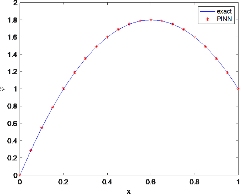
Figure 3: Solution of the 1D problem. Arbitrary units are used for visualization.
C. 2D problem, local residual approach
As a less trivial test case, the following 2D problem has been considered:
| (11) |
The domain is described in Fig. 4, in which . Also in this case, a shallow NN with sigmoidal activation functions has been used. The details of the network are shown in Table 1.
Table 1: Neural network description
| Input dimension | 2 |
|---|---|
| Output dimension | 1 |
| Number of hidden layers | 5 |
| Number of neurons in each hidden layer | 15 |
| Total number of parameters | 1021 |
The hyper-parameters above described have been determined by using a 5-fold cross validation with the number of hidden layers varying from 1 to 7 and with the number of neurons in each hidden layer from 2 to 20. Due to the final number of parameters, the PINN can be classified as a deep network for regression purpose.
Stochastic gradient descent was the minimization algorithm, with random initialization of weights and biases and a learning rate equal to . sampling points were considered to compute the error function on the grid discretizing the domain. In particular, the adopted grid is composed by a set of 300 equally spaced point, in both the and directions, with , as shown in Fig. 5.
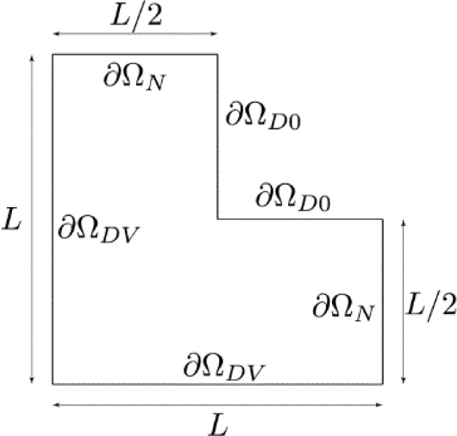
Figure 4: Graphical description of the 2D test case. is the section of boundary where Neumann conditions hold, and the sections where vanishing and non-vanishing Dirichlet conditions hold, respectively.
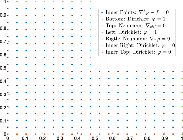
Figure 5: Representation of the grid used to train the PINN or the 2D example.
In case the local residual approach (2)-(4) is followed, the solution obtained after training the PINN is depicted in Fig. 6, while Fig. 7 shows the field evaluated by AD.
The error function training history is shown in Fig. 8. The accuracy of the solution has been properly verified, comparing the obtained potential with the results obtained by a finite element method model implemented on Comsol Multiphysics [23]. For the sake of conciseness, a point-to-point comparison is not shown here, but an integral like comparison (between the energies calculated by both methods) is shown in the next section.
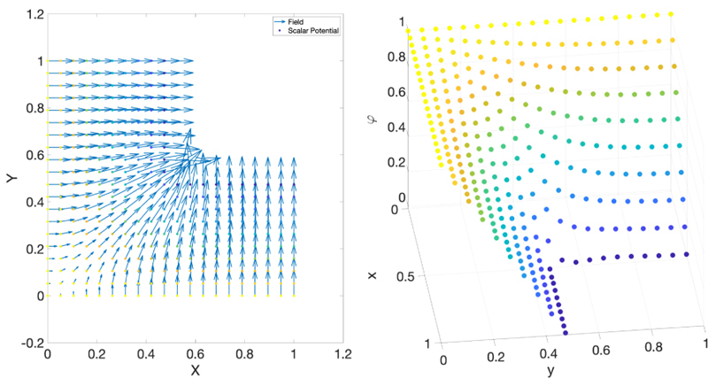
Figure 6: Potential map obtained by the use of the PINN.
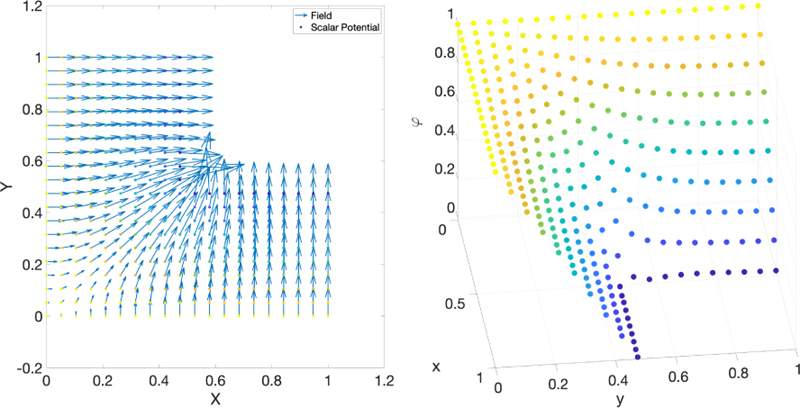
Figure 7: Field as evaluated by the PINN and AD.
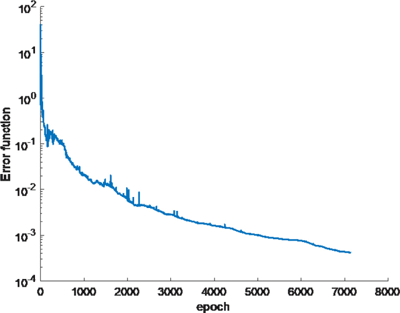
Figure 8: Error function history during training (2D problem).
D. 2D problem, integral error approach
As an intermediate step between the local residual approach and the integral error approach, the behavior of the global energy as a function of the training epoch has been evaluated (Fig. 9). In this case, the “energy” is calculated by using the point values of (obtained by AD), integrated on the relevant support ( in case of a grid point belonging to ). This shows that, in the considered case, the integral formulation leads to the same result, yet being able to treat prospectively also the case of internal discontinuities in the material properties like magnetic permeability. The graph shows that the energy
| (12) |
(with being the magnetic permeability) reaches a value of at the end of the training phase the total energy independently obtained by means of the benchmark FEM is , showing again the good agreement between the PINN and the FEM analysis. It is noteworthy that, in case the integral approach is performed on delta-like expansion functions, the evaluation of the integral approach leads to the same point-wise evaluation as shown in Fig. 5 at the same time, eq. (12) can substitute eq. (4) in the definition of an integral error approach, which would take the meaning of an energy-based approach.
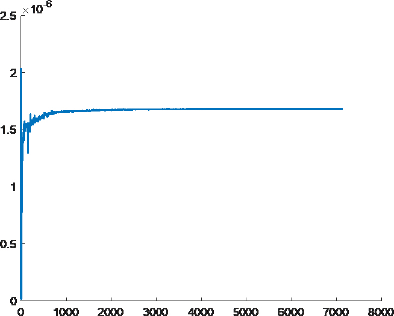
Figure 9: Energy during training (2D problem).
IV. CONCLUSIONS AND OUTLOOK
In this paper, the use of PINN for the resolution of EM problems has been considered. Both local and integral errors, the latter being related to the value of the energy in the domain object of analysis, have been proposed as error functions for the NN training. In the considered examples, both approaches converged during the training phase.
The examples are aimed at showing the effectiveness of energy-based training in particular, the latter is able to easily deal also with problems entailing discontinuities in the distribution of material properties. Moreover, when using a weighted residual formulation rather than the Ritz one, a different choice of the base functions and weight functions would be possible this way, most numerical methods based on weighted residual could be revisited in terms of PINN.
REFERENCES
[1] A. Kovacs, L. Exl, A. Kornell, J. Fischbacher, M. Hovorka, M. Gusenbauer, L. Breth, H. Oezelt, D. Praetorius, D. Suess, and T. Schrefl, “Magnetostatic and micro magnetism with PINNs,” J. of Magnet. and Mag. Mat., vol. 548, 2022.
[2] A. Khan and D. A. Lowther, “Physics informed neural networks for electromagnetic analysis,” IEEE Transactions on Magnetics, vol. 5, no. 9, 2022.
[3] S. Barmada, P. Di Barba, A. Formisano, M. E. Mognaschi, and M. Tucci, “Learning inverse models from electromagnetic measurements data,” Proc. of IGTE Symp. 2022, Graz (Austria), Sep. 18-21, 2022.
[4] M. Raissi, P. Perdikaris, and G. E. Karniadakis, “PINNs: A deep learning framework for solving forward and inverse problems involving nonlinear partial differential equations,” J. Comput. Phys., vol. 378, pp. 686707, 2019.
[5] P. Rumuhalli, L. Udpa, and S. Udpa, “Finite element neural networks for elec. inverse problems,” Rev. Q. Nondestr. Eval., vol. 21, p. 28735, 2002.
[6] W. Tang, T. Shan, X. Dang, M. Li, F. Yang, S. Xu, and J. Wu, “Study on Poissons equation solver based on deep learning technique,” 2017 IEEE El. Design of Adv. Pack. and Syst. Symp., Haining, China, 2018.
[7] Z. Zhang, L. Zhang, Z. Sun, N. Erickson, R. From, and J. Fan, “Study on a Poissons equation solver based on deep learning technique,” Proc. of J. Int. Symp. on Elect. Compat., Sapporo, p. 305308, 2019.
[8] B. Bartlett, “A generative model for computing electromagnetic field solutions,” Stanford CS229 Projects, 233 Stanford, CA, 2018.
[9] J. Lim and D. Psaltis, “MaxwellNet: Physics-driven deep neural network training based on Maxwells equations,” APL Photonics, vol. 7, 2022.
[10] Y. Chen, L. Lu, G. Karniadakis, and L. Negro, “Physics-informed neural net. for inv. problems in nano-optics and metamat,” vol. 28, no. 8, 2020.
[11] L. Lu, R. Pestourie, W. Yao, Z. Wang, F. Verdugo, and S. Johnosn, “Physics-informed neural networks with hard constraints for inverse design,” J. Sci. Comput., vol. 43, no. 6, pp. B1105-B1132, 2021.
[12] S. Wang, Z. Pend, and C. Christodoulou, “Physics-informed deep neural networks for transient electromagnetic analysis,” Antennas and Propagation, vol. 1, pp. 404-412, 2020.
[13] M. Baldan, G. Baldan, and B. Nacke, “Solving 1D non-linear magneto quasi-static Maxwells equations using neural networks,” IET Sci. Meas. Technol., vol. 15, pp. 204217, 2021.
[14] A. Kovacs, L. Exl, A. Kornell, J. Fischbacher, M. Hovorka, M. Gusenbauer, L. Breth, H. Oezelt, D. Praetorius, D. Suess, T. Schref, “Magnetost. and microm. with PINNs,” J. of Magnet. and Magnetic Materials, vol. 548, 2022.
[15] A. Beltran-Pulido, I. Bilionis, and D. Aliprantis, ”PINNs for Solving Parametric Magnetostatic Problems,” IEEE Trans. Energy Conversion, 2022.
[16] M. Baldan, P. Di Barba, and D. A. Lowther, “Physics-informed neural networks for solving inverse electromagnetic problems,” IEEE Trans. Magnetics, vol. 59, no. 5, 2023.
[17] S. H. Rudy, S. L. Brunton, J. L. Proctor, and J. N. Kutz, “Data-driven discovery of partial differential equations,” Sci. Adv., vol. 3, no. 4, Art. no. e1602614, 2017.
[18] Z. Long, Y. Lu, X. Ma, and B. Dong, “PDE-Net: Learning PDEs from data,” in Proc. 35th Int. Conf. Mach. Learn., pp. 3208-3216, 2018.
[19] V. Dwivedi and B. Srinivasan, “Physics informed extreme learning machine (PIELM)—A rapid method for the numerical solution of partial,” Neurocomputing, vol. 391, pp. 96-118, 2020.
[20] S. Mishra, “A machine learning framework for data driven acceleration of computations of differential equations,” Math. Eng., vol. 1, no. 1, pp. 118-146, 2018.
[21] A. G. Baydin, B. A. Pearlmutter, A. A. Radul, and J. M. Siskind, “Automatic differentiation in machine learning: a survey,” J. of Machine Learning Res., vol. 18, no. 153, pp. 1-43, 2018.
[22] O. C. Zienkiewicz and R. Taylor, The Finite Element Method (4th ed.), New York: McGraw-Hill Book Co., 1989.
[23] COMSOL Multiphysics® v. 6.2. www.comsol.com. COMSOL AB, Stockholm, Sweden.
BIOGRAPHIES

Sami Barmada received the M.S. and Ph.D. degrees in electrical engineering from the University of Pisa, Italy, in 1995 and 2001, respectively. He is currently a full professor with the Department of Energy and System Engineering, University of Pisa. He is author and co-author of more than 180 papers in international journals and indexed conferences. His research interests include applied electromagnetics, electromagnetic fields calculation, power line communications, wireless power transfer devices, and nondestructive testing.
Prof. Barmada is an Applied Computational Electromagnetics Society (ACES) Fellow, and he served as ACES president from 2015 to 2017. He is chairman of the International Steering Committee of the CEFC Conference and he has been the general chairman and technical program chairman of numerous international conferences.

Paolo Di Barba is a full professor of electrical engineering in the Department of Electrical, Computer, and Biomedical Engineering, University of Pavia, Pavia, Italy. His current research interests include the computer-aided design of electric and magnetic devices, with special emphasis on the methods for field synthesis and automated optimal design. He has authored or coauthored more than 240 papers, either presented to international conferences or published in international journals, the book Field Models in Electricity and Magnetism (Springer, 2008), the monograph Multiobjective Shape Design in Electricity and Magnetism (Springer, 2010) and the book Optimal Design Exploiting 3D Printing and Metamaterials (2022).

Alessandro Formisano is a full professor at Università della Campania “Luigi Vanvitelli.” His scientific activity started in 1996, in cooperation with several research groups active in the fields of electromagnetic fields and devices (e.g., EdF Paris, TU-Graz, TU-Budapest, TU-Ilmenau, TU-Bucharest, Slovak Academy of Science, Grenoble Univ.), and thermonuclear controlled fusion (KIT, ITER, Fusion For Energy, EURATOM). His interests are electromagnetic fields computation, neural networks, robust design and tolerance analysis, thermonuclear plasmas identification, optimal design, and inverse problems in electromagnetism. He serves as editorial board member or reviewer for the most prestigious journals (IEEE Trans. On Magn., Compel, Sensors, ACES Journal) in the field of numerical computation of electromagnetic fields.

Maria Evelina Mognaschi is associate professor at the University of Pavia (Italy), Department of Electrical, Computer and Biomedical Engineering. Her scientific interests are inverse problems, in particular multi-objective optimization and identification problems in electromagnetism and biological systems. Recently, she investigated the solution of forward and inverse problems in electromagnetics by means of deep learning techniques. She has authored or co-authored more than 120 ISI- or Scopus-indexed papers, either presented to international conferences or published in international journals.

Mauro Tucci received the Ph.D. degree in applied electromagnetism from the University of Pisa, Pisa, Italy, in 2008. Currently, he is a full professor with the Department of Energy and Systems Engineering, University of Pisa. His research interests are machine learning, data analysis, and optimization, with applications in electromagnetism, nondestructive testing, and forecasting.
ACES JOURNAL, Vol. 38, No. 11, 841–848
doi: 10.13052/2023.ACES.J.381102
© 2023 River Publishers