High-precision Solution of Monostatic Radar Cross Section based on Compressive Sensing and QR Decomposition Techniques

Chaofan Shi${}^{\mathbf{\text{1}}}$, Yufa Sun${}^{\mathbf{\text{1*}}}$, Mingrui Ou${}^{\mathbf{\text{1}}}$, Pan Wang${}^{\mathbf{\text{1}}}$, and Zhonggen Wang${}^{\mathbf{\text{2}}}$

¹School of Electronic and Information Engineering
Anhui University, Hefei, 230601, China
1186621445@qq.com, yfsun_ahu@sina.com, 15838288570@163.com, pwangsunny@foxmail.com
*Corresponding Author
²School of Electrical and Information Engineering
Anhui University of Science and Technology, Huainan, 232001, China
zgwang@ahu.edu.cn

Submitted On: August 16, 2023; Accepted On: November 15, 2023

ABSTRACT

In solving the monostatic electromagnetic scattering problem, the traditional improved primary characteristic basis function method (IPCBFM) often encounters difficulties in constructing the reduced matrix due to the long computation time and low accuracy. Therefore, a new method combining the compressed sensing (CS) technique with IPCBFM is proposed and applied to solve the monostatic electromagnetic scattering problem. The proposed method utilizes the characteristic basis functions (CBFs) generated by the IPCBFM to achieve a sparse transformation of the surface-induced currents. Several rows in the impedance matrix and excitation vector are selected as the observation matrix and observation vector. The QR decomposition is adopted as the recovery algorithm to realize the recovery of surface-induced currents. Numerical simulations are performed for cylinder, cube, and almond models, and the results show that the new method has higher solution accuracy, shorter computation time, and stronger solution stability than the traditional IPCBFM. It is worth mentioning that the new method reduces the recovery matrix size and the number of CBFs quantitatively, and provides a novel solution for solving monostatic RCS of complex targets.

Index Terms: compressing sensing, characteristic basis functions, monostatic electromagnetic scattering.

I. INTRODUCTION

The method of moments (MOM) [1] has been a powerful numerical technique widely used for solving electromagnetic scattering problems. However, as the electrical size of the computed target increases, the computational cost becomes unacceptably high. To address this issue, several improved methods have been proposed, including the fast multipole method (FMM) [2], the characteristic basis function method (CBFM) [3–4], the adaptive integration method (AIM) [5], and the adaptive cross approximation (ACA) algorithm [6]. Recently, compressive sensing (CS) technology has been applied to MOM, offering a new solution method. The CS technique in the analysis of electromagnetic scattering problems contains two traditional computational models. The first model is used to decrease the number of incident angles, compressing only the excitation sources [7–8]. The second model involves transforming the dense matrix equation into an underdetermined equation that satisfies the CS framework [9–10]. An underdetermined equation is a system of linear equations with more unknowns than equations. For example, Wang proposed two methods to efficiently analyze the three-dimensional bistatic scattering problem [11–12]. The conventional underdetermined equation [13] computation model is not suited for analyzing monostatic electromagnetic scattering problems. The core problem is that traditional recovery algorithms, such as generalized orthogonal matching pursuit (GOMP) [14] and orthogonal matching pursuit (OMP) [15], are not suitable for the analysis of such problems. When using GOMP or OMP as the recovery algorithm to analyze the monostatic scattering problem, it is necessary to repeat the solution for each incident angle, which increases the computation time. If we can find a suitable recovery algorithm to overcome the repeated solution at each angle, we can fully utilize the advantages of constructing an underdetermined equation computational model, reduce the complexity of the algorithm, and reduce the computation time by compressing the impedance matrix.

The CBFM [4] is an effective method for solving monostatic electromagnetic scattering problems. In [16], the ACA-SVD has been adapted to efficiently generate the characteristic basis functions (CBFs), which reduces both the time of generating the initial CBFs and the singular value decomposition (SVD) time of initial CBFs. In [17], high-level CBFs have been proposed to improve the iterative solution efficiency of CBFM. In [18], a new method of constructing reduced matrix equations is proposed to reduce the time of constructing CBFs. In [19], an improved primary CBFM (IPCBFM) has been proposed to reduce the amount of memory used for the reduced matrix by combining the secondary CBFs with the primary CBFs. While these methods aim to address the monostatic electromagnetic scattering problem by constructing a reduced matrix, the solution often encounters difficulties in solving monostatic electromagnetic scattering problems due to the long computation time and low accuracy.

To overcome the aforementioned issues, a new method called CS-IPCBFM is proposed in this paper. The proposed approach utilizes IPCBFM to generate fewer CBFs that serve as a sparse transformation matrix [10], thereby reducing the dimension of the recovery matrix and accelerating the solution process. Using the QR decomposition [20] algorithm instead of the traditional GOMP algorithm, the recovery matrix equation can be decomposed once, and other incident angles can be solved directly. Therefore, the problem that too many incident angles cause too long solving time can be solved. Several numerical experiments of differently shaped targets are conducted to verify the better computation accuracy and shorter computation time of the CS-IPCBFM.

II. COMPRESSIVE SENSING THEORY

In signal processing and numerous other application domains, signal recovery plays a pivotal role. Successful signal recovery not only effectively suppresses noise but also simplifies the data processing and transmission workflow, and helps to extract the original information, which has a high value in various fields.

If a signal exhibits sparsity in the transform domain, it can be represented using an observation matrix that is uncorrelated with the sparse transformation basis [10]. The signal recovery process primarily consists of the following three parts:

A. Sparse representation

Sparse representation means that the signal has very few non-zero elements in a certain representation, which makes it possible to accurately recover the signal with much less data than traditional sampling, thus achieving efficient signal acquisition and transmission.

Consider a signal $\mathit{X}$ of dimension $N\times 1$. If $\mathit{X}$ is inherently sparse, we can proceed directly to the next phase. For non-sparse signals, it’s crucial to find an optimal sparse transformation matrix, denoted as $\mathbf{\Psi }$ to represent $\mathit{X}$ in its sparse form:

$${\mathit{X}}_{N\times 1}={\mathrm{\Psi }}_{N\times N}{\mathit{\alpha }}_{N\times 1},$$

(1)

where, $\mathbf{\Psi }$ represents the sparse transformation matrix. and $\mathit{\alpha }$ represents the coefficient vector.

B. Measurement matrix design

If the signal ${\mathit{X}}_{N\times 1}$ is sparse, it can be directly observed using the measurement matrix $\mathbf{\Phi }\in {\mathit{R}}^{M\times N}(M<N)$ to obtain a low-dimensional measurement vector ${\mathit{Y}}_{M\times 1}$, which can be expressed as

$${\mathit{Y}}_{M\times 1}={\mathbf{\Phi }}_{M\times N}{\mathit{X}}_{N\times 1}.$$

(2)

If the signal ${\mathit{X}}_{N\times 1}$ is non-sparse, substituting equation (1) into equation (2), the following expression is obtained:

$${\mathit{Y}}_{M\times 1}={\mathbf{\Phi }}_{M\times N}{\mathbf{\Psi }}_{N\times N}{\mathit{\alpha }}_{N\times 1}={\mathbf{\Theta }}_{M\times N}{\mathit{\alpha }}_{N\times 1}$$

(3)

where ${\mathbf{\Theta }}_{M\times N}$ is the recovery matrix.

C. Signal recovery

If the projection of the signal ${\mathit{X}}_{N\times 1}$ onto ${\mathbf{\Psi }}_{N\times N}$ has only $k$ non-zero elements, signal ${\mathit{X}}_{N\times 1}$ is referred to as $k$ sparse. The high-dimensional original signal ${\mathit{X}}_{N\times 1}$ is reconstructed by utilizing a low-dimensional observation vector ${\mathit{Y}}_{M\times 1}$. when the restricted isometry property (RIP) [21] is satisfied and the value of $M$ satisfies $M⩾O(k\log (N/k))$, $\mathit{\alpha }$ can be recovered with high probability by solving an $l_1$-norm optimization problem denoted as

$$\widehat{\mathit{\alpha }}=\arg \min {\parallel \mathit{\alpha }\parallel }_1\text{s.t}\mathbf{\Theta }\mathit{\alpha }=\mathit{Y},$$

(4)

where $\parallel \cdot {\parallel }_1$ denotes the $l_1$ norm [22]. In this paper, the QR decomposition is chosen as the recovery algorithm for solving $\widehat{\mathit{\alpha }}$. Finally, the original signal $\mathit{X}$ is obtained by substituting $\widehat{\mathit{\alpha }}$ into equation (1).

A simple example is provided here for illustration. Consider a signal $x=[2,3,1,4,2]$. Upon applying the discrete cosine transform (DCT) to $x$, we obtain $s=DCT[x]=[12,-1.4,0.6,-3.7,-1.5]$. Assuming that the threshold is 1.5, the coefficient whose absolute value is higher than the threshold is retained, thus $\widehat{s}=[12,0,0,-3.7,0]$. Applying the inverse DCT to these coefficients, we reconstruct the signal as $\widehat{x}=[2.2,2.9,1.2,3.8,1.9]$.

III. THE APPLICATION OF CS IN THE CONSTRUCTION OF AN UNDERMINED EQUATION

The CBFM divides the target into M blocks, with each block discretized into $N_i$ units. Using $N_{pws}$ plane waves as excitations to generate primary characteristic basis functions (PCBFs). Let $P_{\theta }$ and $P_{\phi }$ represent the number of samples in the $\theta$ and $\phi$ directions, respectively. The total number of plane waves is $N_{pws}=2P_{\theta }{P}_{\phi }$. The PCBFs ${\mathit{J}}_{ii}^P$ for the block $i$ is defined asfollows:

$${\mathit{Z}}_{ii}{\mathit{J}}_{ii}^P(\theta )={\mathit{E}}_i^{N_{pws}}(\theta )(i=1,2,\mathrm{\dots },\mathrm{M}),$$

(5)

where ${\mathit{Z}}_{ii}$ is the $N_i\times N_i$ impedance matrix of self-interaction within the block $i,{\mathit{E}}_i^{N_{pws}}$ is the matrix containing excitation vectors with size $N_i\times N_{pws},\theta$ is the incident angle, and ${\mathit{J}}_{ii}^P$ is the $N_i\times N_{pws}$ matrix to be obtained. The secondary characteristic basis functions ${\mathit{J}}_{ij}^S$ indicates the mutual interaction component between block $i$ and $j$. The definition of ${\mathit{J}}_{ij}^S$ for block $i$ is as follows:

$${\mathit{Z}}_{ii}{\mathit{J}}_{ij}^S(\theta )=-{\mathit{Z}}_{ij}{\mathit{J}}_{ij}^P(\theta )(j=1,2,\mathrm{\dots },\mathrm{M})$$

(6)

where, ${\mathit{Z}}_{ij}$ is the $N_i\times N_j$ mutual impedance between the subdomains $i$ and $j,{\mathit{J}}_{ij}^S$ is the $N_i\times N_{pws}$ matrix. Combining equation (6) and equation (7), the IPCBFs ${\mathit{J}}_i^{IP}$ can be obtained and represented as

	${\mathit{Z}}_{ii}{\mathit{J}}_{ii}^P(\theta )+{\displaystyle \sum _{j=1(j\ne i)}^M}{\mathit{Z}}_{ii}{\mathit{J}}_{ij}^S(\theta )$
	$={\mathit{Z}}_{ii}{\displaystyle \sum _{j=1}^M}{\mathit{J}}_{ij}^{P,S}(\theta )={\mathit{Z}}_{ii}{\mathit{J}}_i^{IP}(\theta ),$
	$={\mathit{E}}_i^{N_{pws}}(\theta )-{\displaystyle \sum _{j=1(j\ne i)}^M}{\mathit{Z}}_{ij}{\mathit{J}}_{jj}^P(\theta )$		(7)

where ${\mathit{J}}_i^{IP}$ is the $N_i\times N_{pws}$ matrix, ${\mathit{J}}_{ij}^{P,S}$ includes both ${\mathit{J}}_{ii}^P$ and ${\mathit{J}}_{ij}^S$. In the IPCBFM [19], due to the selection of a large number of incident waves $N_{pws}$, the generated matrix ${\mathit{J}}_i^{IP}$ contains redundant information. The singular value decomposition (SVD) technique is employed to decompose ${\mathit{J}}_i^{IP}$. After SVD processing, a set of ${\widehat{\mathit{J}}}_i^{IP}$ is generated that is independent of the incident angle. The ${\mathit{J}}_i^{IP}$ can be represented as

$${\mathit{J}}_i^{IP}=\mathit{U}\sum {\mathit{V}}^T,$$

(8)

where $U$ and $V$ are unitary matrices, $\mathrm{\Sigma }$ is a semi-positive definite diagonal matrix. SVD is performed on matrix ${\mathit{J}}_i^{IP}$ using a threshold value $\epsilon ={\sigma }_M/{\sigma }_1$. Singular values greater than $\epsilon$ are retained, while values less than that are discarded, resulting in the matrix ${\widehat{\mathit{J}}}_i^{IP}$. Assuming there are $K_i$ retained IPCBFs in the $i$-th subdomain, ${\widehat{\mathit{J}}}_i^{IP}$ can be denoted as

$${\widehat{\mathit{J}}}_i^{IP}=\sum _{k=1}^{K_i}{\alpha }_i^k{\mathit{J}}_i^k,(i=1,2,\mathrm{\dots },M),$$

(9)

where ${\alpha }_i^k$ is the undetermined coefficient of the IPCBFs. The surface-induced current of the entire target can be denoted as

	$\mathit{J}=\left[\begin{array}{c}\hfill {\widehat{\mathit{J}}}_1^{IP}\hfill \\ \hfill {\widehat{\mathit{J}}}_2^{IP}\hfill \\ \hfill \mathrm{⋮}\hfill \\ \hfill {\widehat{\mathit{J}}}_{\mathrm{M}}^{IP}\hfill \end{array}\right]={\displaystyle \sum _{k=1}^{K_1}}{\alpha }_1^{\mathrm{k}}\left[\begin{array}{c}\hfill {\mathit{J}}_1^k\hfill \\ \hfill [0]\hfill \\ \hfill \mathrm{⋮}\hfill \\ \hfill [0]\hfill \end{array}\right]+\mathrm{\cdots }+{\displaystyle \sum _{k=1}^{K_M}}{\alpha }_{\mathrm{M}}^{\mathrm{k}}\left[\begin{array}{c}\hfill [0]\hfill \\ \hfill [0]\hfill \\ \hfill \mathrm{⋮}\hfill \\ \hfill {\mathit{J}}_{\mathrm{M}}^k\hfill \end{array}\right]$
	$=\left[\begin{array}{ccccc}\hfill {\mathit{J}}_1^C\hfill & \hfill \mathrm{\cdots }\hfill & \hfill 0\hfill & \hfill \mathrm{\cdots }\hfill & \hfill 0\hfill \\ \hfill \mathrm{⋮}\hfill & \hfill \mathrm{\ddots }\hfill & \hfill \mathrm{⋮}\hfill & \hfill \mathrm{\ddots }\hfill & \hfill \mathrm{⋮}\hfill \\ \hfill [0]\hfill & \hfill \mathrm{\cdots }\hfill & \hfill {\mathit{J}}_i^C\hfill & \hfill \mathrm{\cdots }\hfill & \hfill [0]\hfill \\ \hfill \mathrm{⋮}\hfill & \hfill \mathrm{\ddots }\hfill & \hfill \mathrm{⋮}\hfill & \hfill \mathrm{\ddots }\hfill & \hfill \mathrm{⋮}\hfill \\ \hfill [0]\hfill & \hfill \mathrm{\cdots }\hfill & \hfill [0]\hfill & \hfill \mathrm{\cdots }\hfill & \hfill {\mathit{J}}_M^C\hfill \end{array}\right]\left[\begin{array}{c}\hfill {\alpha }_1^C\hfill \\ \hfill \mathrm{⋮}\hfill \\ \hfill {\alpha }_1^C\hfill \\ \hfill \mathrm{⋮}\hfill \\ \hfill {\alpha }_M^C\hfill \end{array}\right]={\widehat{\mathit{J}}}^C\mathit{\alpha },$		(10)

where ${\alpha }_i^C=\left[\begin{array}{cccc}{\alpha }_i^1\hfill & {\alpha }_i^2\hfill & \mathrm{\cdots }\hfill & {\alpha }_i^{K_i}\hfill \end{array}\right],{\mathit{J}}_i^C=\left[\begin{array}{cccc}{\mathit{J}}_i^1\hfill & {\mathit{J}}_i^2\hfill & \mathrm{\cdots }\hfill & {\mathit{J}}_i^{K_i}\hfill \end{array}\right]$.

In the MOM, the surface integral equation is discretized by the Rao-Wilton-Glisson (RWG) basis function into a matrix equation as follows:

$${\mathit{Z}}_{N\times N}\cdot {\mathit{J}}_{N\times 1}(\theta )={\mathit{E}}_{N\times 1}(\theta )$$

(11)

where ${\mathit{Z}}_{N\times N}$ is the impedance matrix, ${\mathit{J}}_{N\times 1}$ is the surface-induced currents, ${\mathit{E}}_{N\times 1}$ is an excitation vector, $N$ represents the number of the RWG basis functions. The measurement matrix ${\tilde{\mathit{Z}}}_{L\times N}$ and measurement vector ${\tilde{\mathit{E}}}_{L\times 1}$ are created by randomly selecting $L(L<N)$ rows from matrices ${\mathit{Z}}_{N\times N}$ and ${\mathit{E}}_{N\times 1}$, respectively. An underdetermined equation is created as

$${\tilde{\mathit{Z}}}_{L\times N}{\mathit{J}}_{N\times 1}(\theta )={\tilde{\mathit{E}}}_{L\times 1}(\theta ).$$

(12)

By substituting equation (10) into equation (12), an overdetermined system of equations is obtained:

$${\tilde{\mathit{Z}}}_{L\times N}{\widehat{\mathit{J}}}_{N\times K}^C{\mathit{a}}_{K\times 1}={\mathbf{\Theta }}_{L\times K}{\mathit{a}}_{K\times 1}={\tilde{\mathit{E}}}_{L\times 1}(\theta ),$$

(13)

where ${\mathbf{\Theta }}_{L\times K}$ is the recovery matrix, ${\widehat{\mathit{J}}}_{N\times K}^C$ is the sparse transformation matrix. $K(K<L)$ represents the total number of retained IPCBFs across all subdomains.

Firstly, the conventional GOMP is employed as the recovery algorithm to solve equation (13), and this method is referred to as CS-IPCBFM-1 in this paper. Where the GOMP algorithm is as follows:

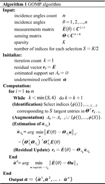
However, as depicted in Algorithm 1, this method requires repeated calculations at each incidence angle, making the computation time increase.

Next, the least squares fitting method is employed to solve equation (13) and this computation method is called CSIPCBFM-2 in this paper. Where the least squares fitting algorithm is as follows:

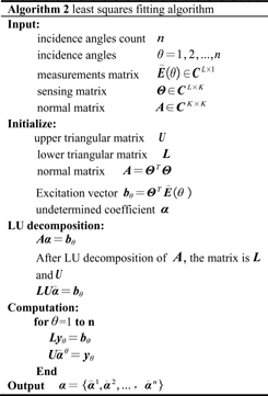
As described in Algorithm 2, the method first performs the LU decomposition of $\mathit{A}$ and then performs the solution process, avoiding repeated solutions at each incident angle.

Finally, the QR decomposition is used as the recovery algorithm to solve equation (13), and this method is called CS-IPCBFM in this paper. Where the QR decomposition algorithm is as follows:

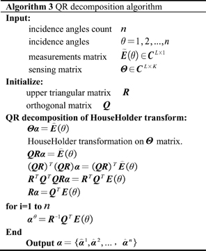
As described in Algorithm 3, the QR decomposition method is used to decompose the recovery matrix $\mathit{\theta }$ and then solve it, avoiding repeated solutions at each incident angle.

IV. COMPLEXITY ANALYSIS

To provide a clear comparison of the complexity between IPCBFM and CS-IPCBFM, a focused analysis was conducted solely on these two methods. CS-IPCBFM-1 and CS-IPCBFM-2, on the other hand, were validated via numerical simulations. The calculation processes for IPCBFM and CS-IPCBFM consist of three steps: filling the impedance matrix, constructing IPCBFs, and solving the radar cross section (RCS).

Since both filling the impedance matrix and constructing IPCBFs are identical for IPCBFM and CS-IPCBFM, this section focuses solely on comparing the complexities of the RCS-solving steps.

The RCS solution process of IPCBFM involves constructing and solving the reduced matrix equation, whose combined complexity is $O\left(K^2{N}_i^2+K^3\right)$. In CS-IPCBFM, the RCS solution process includes the construction of the recovery matrix and the solution of equation (13), whose combined complexity is $O\left(NLK+K^2+LK\right)$. Since $NL<K{N}_i^2$, and $K+L<K^2$, the RCS calculation time of CS-IPCBFM will be shorter than that of IPCBFM.

V. NUMERICAL RESULTS

To validate the effectiveness of the proposed method, three models of cylinder, cube, and almond are simulated. Where, the cylinder model with fewer unknowns was used to compare IPCBFM, CS-IPCBFM-1, and CS-IPCBFM methods. While the cube and almond models with more unknowns were used to compare IPCBFM, CS-IPCBFM-2, and CS-IPCBFM methods. The results were computed using an AMD Ryzen $75800\mathrm{H}$ with Radeon Graphics 3.20 GHz and 64.0 GB RAM, and the simulations were compiled using Visual Studio 2022RC. Additionally, all examples utilized a double-precision floating point. The root-meant-square error of the target monostatic RCS is defined as

	$\mathit{E}\mathit{r}\mathit{r}(\%)=100\%$
	$\times \sqrt{{\displaystyle \frac{1}{N}}{\displaystyle \sum _{i=1}^N}{\left|\mathit{R}C{S}_i-\mathit{R}\mathit{C}{\mathit{S}}_i^{\mathit{\text{MOM}}}\right|}^2/{\left|\mathit{R}\mathit{C}{\mathit{S}}_i^{\mathit{\text{MOM}}}\right|}^2}.$		(14)

Firstly, the monostatic RCS of a perfect electrical conductor (PEC) cylinder with a length of $2\mathrm{m}$ and radius of 0.3 $\mathrm{m}$ at $800\mathrm{M}\mathrm{H}\mathrm{z}$ is calculated. The angle of incidence is set to $\theta =0^{\circ }-{180}^{\circ },\phi =0^{\circ }$. The geometry was divided into 5046 triangular patches, resulting in 14,161 unknowns. Subsequently, the cylinder was segmented into 12 blocks, with each block extending $\mathrm{\Delta }=0.15\lambda$ in all directions, which increased the number of unknowns to 25,966. When the threshold $\epsilon$ is set to 0.01, a total of 755 IPCBFs are obtained. The monostatic RCS values of MOM, IPCBFM, CSIPCBFM-1, and CS-IPCBFM are found to be highly consistent, as depicted in Fig. 1.

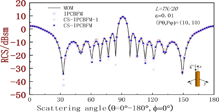
Figure 1: HH polarization monostatic RCS of cylinder.

As the number of rows $L$ increases, the computation time of CS-IPCBFM and CS-IPCBFM-1 is shown in Figs. 2 and 3, respectively. The computation time of IPCBFM is 18.481 s, as depicted in Fig. 2. As can be seen from Figs. 2 and 3, when $20L/N$ is less than 11, CS-IPCBFM has the lowest computation time compared to IPCBFM and CSIPCBFM-1. The RCS error of the IPCBFM, CS-IPCBFM-1 and CS-IPCBFM is shown in Fig. 4. When 20L/N is greater than 6, the CS-IPCBFM has the highest accuracy compared to the IPCBFM and CS-IPCBFM-1.

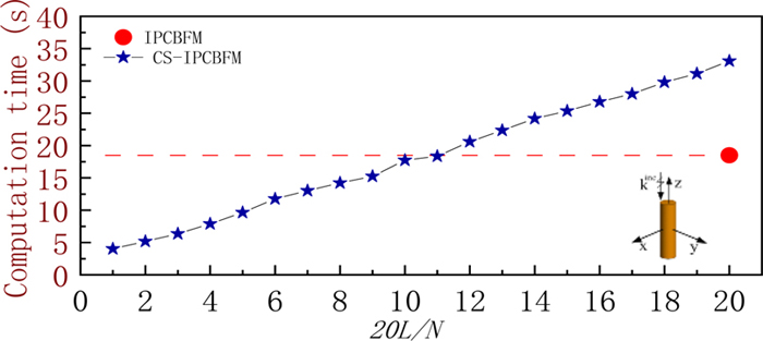
Figure 2: Computation time of cylinder for different $L$.

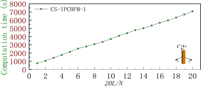
Figure 3: Computation time of cylinder for different $L$.

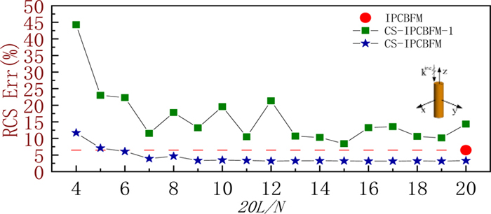
Figure 4: RCS Err of the cylinder for different $L$.

Next, the monostatic RCS of a PEC cube with a length of $1\mathrm{m}$ at $800\mathrm{M}\mathrm{H}\mathrm{z}$ is calculated. The angle of incidence is set to $\theta =0^{\circ }-{180}^{\circ },\phi =0^{\circ }$. The cube is discretized into 13,980 triangular patches producing 25,981 unknowns. When the target is divided into 8 blocks, with each block extending by $\mathrm{\Delta }=0.15\lambda$ in all directions, the number of unknowns increases to 46,951. Furthermore, a total of 789 IPCBFs are obtained when the SVD threshold is set to $\epsilon =0.02$. The monostatic RCS values of MOM, IPCBFM, CS-IPCBFM-2, and CS-IPCBFM are found to be highly consistent, as depicted in Fig. 5. As the SVD threshold $\epsilon$ increases, the RCS error and computation time of IPCBFM and CSIPCBFM is shown in Figs. 6 and 7. From these figures, it can be seen that CS-IPCBFM has a shorter computation time and lower RCS error compared to IPCBFM. As the number of rows $L$ increases, the RCS error and computation time of the CS-IPCBFM and CS-IPCBFM-2 are shown in Figs. 8 and 9. While the RCS error and computation time of IPCBFM are 2.0632% and 189.657s, as depicted in Figs. 8 and 9, respectively. As can be seen from Figs. 8 and 9, when $20\mathrm{L}/\mathrm{N}$ is less than 15, the CS-IPCBFM has a shorter computation time compared to IPCBFM. When $20\mathrm{L}/\mathrm{N}$ is greater than 3, the accuracy of CS-IPCBFM is comparable to that of IPCBFM and better than that of CS-IPCBFM-2.

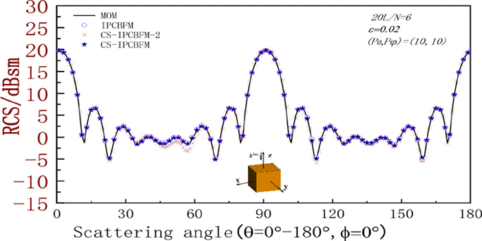
Figure 5: HH polarization monostatic RCS of the cube.

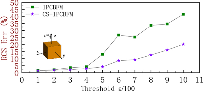
Figure 6: RCS Err of the cube for different $\epsilon$.

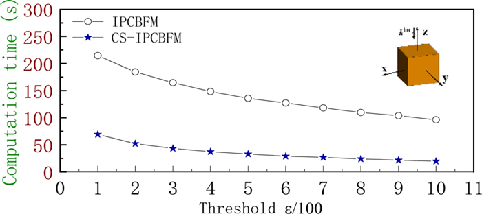
Figure 7: Computation time of the cube for different $\epsilon$.

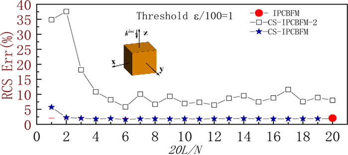
Figure 8: RCS Err of the cube for different $L$.

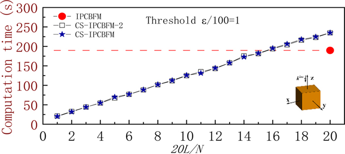
Figure 9: Computation time of the cube for different $L$.

Finally, the monostatic RCS of a PEC almond with a length of $252.374\mathrm{mm}$ at a frequency of $7\mathrm{G}\mathrm{H}\mathrm{z}$ is computed. The target is divided into 8 blocks, and each block is extended by $\mathrm{\Delta }=0.15\lambda$ in all directions, increasing the number of unknowns to 62,653. A total of 710 IPCBFs are obtained when the threshold $\epsilon =0.01$. The monostatic RCS of MOM, IPCBFM, and CS-IPCBFM under horizontal polarizations are found to be highly consistent, and the monostatic RCS of CS-IPCBFM-2 is poor, as depicted in Fig. 10. Finally, the influence of different incident plane wave numbers on the stability of IPCBFM and CS-IPCBFM is investigated. The calculation time and RCS error for various numbers of incident waves are shown in Table 1.

Table 1: Calculation time and RCS error of the almond for various numbers of incident waves

Method	$({\mathit{P}}_{\theta },{\mathit{P}}_{\phi })$	Computation Time (s)	RCS Err (%)
IPCBFM	$(5,5)$	95.439	47.8028
CS-IPCBFM		48.922	26.3877
IPCBFM	$(6,6)$	145.945	43.1824
CS-IPCBFM		67.16	24.8070
IPCBFM	$(7,7)$	200.084	31.4387
CS-IPCBFM		84.298	7.9510
IPCBFM	$(8,8)$	255.595	7.8126
CS-IPCBFM		99.567	4.9569
IPCBFM	$(9,9)$	265.909	6.9566
CS-IPCBFM		107.044	3.0830
IPCBFM	$(10,10)$	291.401	3.7763
CS-IPCBFM		114.989	2.1990

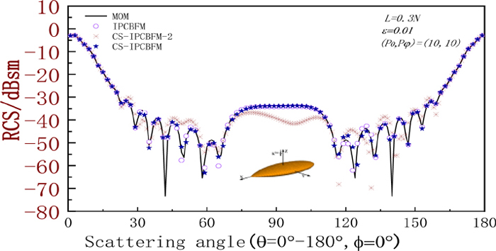
Figure 10: HH polarization monostatic RCS of the almond.

Table 2: Comparison of calculation time, RCS Err, and memory consumption

Model	Method	Impedance Matrix Filling Time (s)	IPCBFs Generation (s)	Solving Time (s)	Total Time (s)	RCS Err (%)	Memory (GB)
Cylinder	IPCBFM			18.481	304.899	6.4736	4.876
	CS-IPCBFM-1	23.194	263.224	2794.45	3080.868	11.5301	4.978
	CS-IPCBFM			13.013	299.431	3.9032	4.473
Cube	IPCBFM			164.685	2367.29	6.6891	17.3826
	CS-IPCBFM-2	72.884	2129.621	42.182	2244.33	36.0286	15.341
	CS-IPCBFM			43.322	2245.93	4.7641	15.324
Almond	IPCBFM			291.401	5540.687	3.7763	39.918
	CS-IPCBFM-2	153.876	5095.41	113.632	5362.918	14.8080	36.831
	CS-IPCBFM			114.989	5364.275	2.1990	39.561

It can be seen from Table 1 that the accuracy stability of the method proposed in this paper is better than that of IPCBFM. The computation time and RCS error of the simulation examples in Figs. 1, 5, and 10 are shown in Table 2. The results show that CS-IPCBFM has a shorter computation time and the highest accuracy in calculating the monostatic RCS.

VI. CONCLUSION

To improve the efficiency and accuracy of IPCBFM, we integrated CS with IPCBFM and refined the conventional CS recovery algorithm. In comparison to IPCBFM, CS-IPCBFM-1 with traditional recovery algorithm has some lag in speed and accuracy, CS-IPCBFM-2 with the least square fitting achieves faster calculation, but the accuracy is compromised, CS-IPCBFM with QR decomposition not only excels in both speed and precision but also offers superior stability.

ACKNOWLEDGMENT

This work was supported in part by the National Natural Science Foundation of China under Grant 62071004 and the Project of Anhui Provincial Natural Science Foundation under Grant no. 2108085MF200.

REFERENCES

[1] R. F. Harrington, Field Computation by Moment Methods, Malabar, Fla.: R. E. Krieger, 1968.

[2] R. Coifman, V. Rokhlin, and S. Wandzura, “The fast multipole method for the wave equation: A pedestrian prescription,” IEEE Antennas and Propagation Magazine, vol. 53, no. 3, pp. 7-12,1993.

[3] V. A. Prakash and R. Mittra, “Characteristic basis function method: A new technique for efficient solution of method of moments matrix equations,” Microwave and Optical Technology Letters, vol. 36, pp. 95-100, 2002.

[4] E. Lucente, A. Monorchio, and R. Mittra, “An iteration-free MoM approach based on excitation independent characteristic basis functions for solving large multiscale electromagnetic scattering problems,” IEEE Transactions on Antennas and Propagation, vol. 56, pp. 999-1007, 2008.

[5] E. Bleszynski, M. Bleszynski, and T. Jaroszewicz, “Adaptive integral method for solving large-scale electromagnetic scattering and radiation problems,” Radio Science, vol, 31, pp. 1225-1251, 1996.

[6] Z. Liu, R. Chen, J. Chen, and Z. Fan, “Using adaptive cross approximation for efficient calculation of monostatic scattering with multiple incident angles,” Applied Computational Electromagnetics Society (ACES) Journal, vol. 26, pp. 325-333, 2011.

[7] M. S. Chen, F. L. Liu, H. M. Du, and X. L. Wu, “Compressive sensing for fast analysis of wide-angle monostatic scattering problems,” IEEE Antennas and Wireless Propagation Letters, pp. 1243-1246, 2011.

[8] S. R. Chai and L. X. Guo. “A new method based on compressive sensing for monostatic scattering analysis,” Microwave and Optical Technology Letters, vol, 10, pp. 2457-2461, 2015.

[9] E. J. Candes, T. Tao, “Near-optimal signal recovery from random projections: Universal encoding strategies,” IEEE Transactions on Information Theory, vol, 52, pp. 5406-5425, 2006.

[10] D. L. Donoho, “Compressed sensing,” IEEE Trans. Inf. Theory, vol. 52, no. 4, pp. 1289-1306, 2006.

[11] Z. G. Wang, W. Y. Nie, and H. Lin. “Characteristic basis functions enhanced compressive sensing for solving the bistatic scattering problems of three-dimensional targets,” Microwave and Optical Technology Letters, vol. 62, pp, 3132-3138,2020.

[12] Z. G. Wang, P. Wang, Y. Sun, and W. Nie, “Fast analysis of bistatic scattering problems for three-dimensional objects using compressive sensing and characteristic modes,” IEEE Antennas and Wireless Propagation Letters, vol. 21, pp. 1817-1821, 2022.

[13] A. M. Bruckstein, D. L. Donoho, and M. Elad, “From sparse solutions of systems of equations to sparse modeling of signals and images,” SIAM Review, vol. 51, pp. 34-81, 2009.

[14] J. Wang, S. Kwon, and B. Shim, “Generalized orthogonal matching pursuit,” IEEE Transactions on Signal Processing, vol. 60, pp. 6202-6216, 2012.

[15] J. A. Tropp and A. C. Gilbert, “Signal recovery from random measurements via orthogonal matching pursuit,” IEEE Trans. Inf. Theory, vol. 53, pp. 4655-4666, Dec. 2007.

[16] X. Chen, C. Gu, Z. Niu, Y. Niu, and Z. Li, “Efficient iterative solution of electromagnetic scattering using adaptive cross approximation enhanced characteristic basis function method,” IET Microwaves, Antennas & Propagation, vol. 9, pp. 217-223,2015.

[17] E. García, C. Delgado, and F. Cátedra, “A novel and efficient technique based on the characteristic basis functions method for solving scattering problems,” IEEE Trans. Antennas Propag., vol. 67, pp. 3241-3248, 2019.

[18] Z. G. Wang, C. Qing, and W. Y. Nie, “Novel reduced matrix equation constructing method accelerates iterative solution of characteristic basis function method,” Applied Computational Electromagnetics Society (ACES) Journal, vol. 34, pp. 1814-1820, Dec. 2019.

[19] T. Tanaka, Y. Inasawa, and Y. Nishioka, “Improved primary characteristic basis function method for monostatic radar cross section analysis of specific coordinate plane,” IEICE Transactions on Electronics, vol. E99-C, pp. 2835, 2016.

[20] C. R. Goodall. “Computation using the QR decomposition,” Handbook of Statistics, vol. 9, pp. 467-508, 1993.

[21] E. J. Candes. “The restricted isometry property and its implications for compressed sensing,” Comptes Rendus Mathematique, vol. 346, pp. 589-592, 2008.

[22] R. Baraniuk, “A lecture on compressive sensing,” IEEE Signal Processing Magazine, vol. 24, pp. 181-121, 2006.

BIOGRAPHIES

Chaofan Shi was born in Xinxiang Henan, China in 1996. He received his B.S. degree from Anyang Institute of Technology in 2020. He is currently pursuing a master’s degree in the School of Electronic and Information Engineering at Anhui University. His research interests mainly focus on electromagnetic scattering.

Yufa Sun was born in 1966. He received the B.S. and M.S. degrees in radio physics from Shandong University, in 1988 and 1991, respectively, and the Ph.D. degree in electromagnetic field and microwave technology from the University of Science and Technology of China, in 2001. Since 1991, he has been a faculty member with Anhui University, Anhui, China, where he is currently a full professor with the School of Electronic and Information Engineering. He was a visiting scholar with the City University of Hong Kong, from 2002 to 2003, and a postdoctoral researcher with the University of Science and Technology of China, from 2003 to 2006. His research interests include electromagnetic scattering and target recognition, computational electromagnetics, and antenna theory and technology.

Mingrui Ou was born in Bengbu, Anhui, China in 1991. He received his B.S. degree from Zhengzhou University of Light Industry in 2013. He is currently pursuing a master’s degree in the School of Electronic and Information Engineering at Anhui University. His research interests mainly focus on electromagnetic scattering.

Pan Wang was born in Huaibei, Anhui, China, in 1989. He received his master’s degree from Anhui University of Science and Technology in 2023. He is currently pursuing a Ph.D. degree in the School ofElectronic and Information Engineering at Anhui University. His research interests mainly focus on computational electromagnetics.

Zhonggen Wang received the Ph.D. degree in electromagnetic field and microwave technique from the Anhui University of China (AHU), Hefei, P. R. China, in 2014. Since 2014, he has been with the School of Electrical and Information Engineering, Anhui University of Science and Technology. His research interests include computational electromagnetics, array antennas, and reflect arrays.

ACES JOURNAL, Vol. 38, No. 8, 616–624
doi: 10.13052/2023.ACES.J.380809
© 2023 River Publishers

ABSTRACT

I. INTRODUCTION

II. COMPRESSIVE SENSING THEORY

A. Sparse representation

B. Measurement matrix design

C. Signal recovery

III. THE APPLICATION OF CS IN THE CONSTRUCTION OF AN UNDERMINED EQUATION

IV. COMPLEXITY ANALYSIS

V. NUMERICAL RESULTS

VI. CONCLUSION

ACKNOWLEDGMENT

REFERENCES

BIOGRAPHIES