Analytical Model of an E-core Driver-pickup Coils Probe Applied to Eddy Current Testing of Multilayer Conductor

Siquan Zhang

Department of Electrical and Automation
Shanghai Maritime University, Shanghai, 201306, China
sqzhang@shmtu.edu.cn

Submitted On: August 30, 2023; Accepted On: December 20, 2023

ABSTRACT

An analytical model of an E-core driver-pickup coils probe located above a multilayer conductor containing a hidden cylindrical conductor is presented. The truncated region eigenfunction expansion (TREE) method is used to deal with the axial symmetry problem, and the closed-form final expression of the induced voltage in the pickup coil is derived. The changes of the induced voltage in the pickup coil due to the hidden cylindrical conductor are examined and calculated in Mathematica. Experiments and finite element simulations are performed and the results are compared with the analytical results, and they are in good agreement.

Keywords: Analytical model, cylindrical conductor, E-core driver-pickup coils probe, eddy current testing, induced voltage.

I. INTRODUCTION

In the aviation, petrochemical, nuclear power, and other industries, nondestructive testing and evaluation (NDT&E) methods are extensively used to acquire information about important components and structures, which is of great significance to ensure the normal operation of equipment and prevent accidents. Eddy current testing (ECT) is a widely used NDT method for detecting conductor defects due to its distinct advantages, such as non-contact, high sensitivity, and low cost. If the ECT probe is an absolute coil probe, the information obtained is the coil impedance or coil impedance change [1–3]. If the probe consists of a driver coil and a pickup coil, an induced voltage will be generated in the pickup coil.

The purpose of many practical ECT is to find the characteristics of conductive materials or reconstruct the shape of defect in the conductor by measuring changes of the coil impedance or changes of the induced voltage in pickup coils [4–6]. In the defect inversion operation [7–8], a lot of time is consumed in the forward model for repeated computations. Therefore, a fast and accurate forward model is very important for conductive defect evaluation. In general, the analytical model has the advantages of fast calculation speed and high accuracy compared with the finite element method. The traditional ECT analytical models proposed by Dodd and Deeds, whose final expressions are in integral form, have been widely used in ECT for more than fifty years [9]. Later, Theodoulidis proposed the truncated region eigenfunction expansion (TREE) method, which can obtain the expression of response in the form of series [10]. Compared with traditional integral model, one of the most important advantages of the TREE method is its fast calculation speed.

Coils are usually combined with ferrite cores to form a magnetic core probe, such as I-core, E-core, and T-core probes. The magnetic core has the function of concentrating the magnetic field, reducing flux leakage and shielding external electromagnetic interference. Therefore, in ECT, the sensitivity of a ferrite core coil is higher than that of an air core coil [11–12]. Among various magnetic cores, E-core has been widely used due to its superior performance.

In this paper, as shown in Fig. 1, the analytical model of an E-core probe placed over a layered conductor is investigated. The probe consists of two coils, an inner coil and an outer coil, both surrounding the column of the E-core with a circular air gap. If one of the coils is selected as the excitation coil and the other as the pickup coil, an E-core driver-pickup probe is formed. If the inner and outer coils are connected in series, they can also form an absolute E-core probe. For the case of an absolute cored coil probe located above an infinite layered conductor, on a multilayer conductor containing air hole, or on a multilayer conductive disk, many scholars have conducted extensive research on their analytical models and derived expressions of the coil impedance of the E-core probe with air gap in various cases [12–15]. However, the analytical model of an E-core probe consisting of an excitation coil and a pickup coil above a multilayer conductor containing a hidden cylindrical conductor has not been examined. In some special applications, driver-pickup coils probes have advantages over absolute coil probes, and the solution method for a multilayer half-space conductor containing a hidden cylindrical conductor is different from that for a multilayer conductor with air hole, so it is necessary to further investigate its analytical model.

II. SOLUTION

The analytical model shown in Fig. 2 (a) is first analyzed, a filamentary driver coil c${}_d$and a filamentary pickup coil c${}_p$. The two filamentary coils are on the same plane, but have different radii, and are both wound around the column of an E-core with a circular air gap. The probe is located above four layers of non-magnetic conductors, the second layer is a hidden cylindrical conductor with radius c, and the remaining layers are half-space conductors. From top to bottom, the conductivities of each layer of conductors are $\sigma$${}_6$, $\sigma$${}_7$, $\sigma$${}_8$, and $\sigma$${}_9$,respectively. The plane z = 0 coincides with the upper surface of the conductor. The whole problem region is truncated into a cylinder with radius b in the radial direction, and the homogeneous Dirichlet condition is applied to the magnetic vector potential on the truncation boundary.

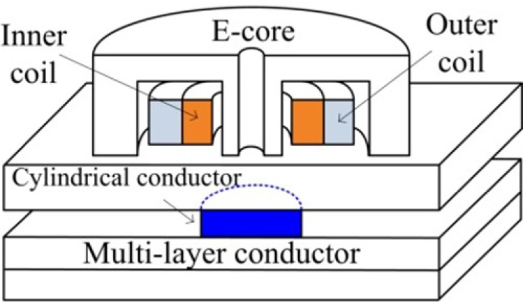
Figure 1: E-core driver and pickup coils probe located above layered conductor containing a hidden cylindrical conductor.

According to the problem geometry, nine regions are formed along the z-axis in Fig. 2 (a). The cylindrical conductor is hidden in region 7. For other regions, the eigenvalues of each region can be defined and calculated in a similar way as discussed for E-core coil in the references [12–14], and will not be repeated here.

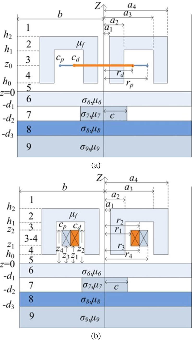
Figure 2: Axially symmetric E-core (a) filamentary and (b) rectangular cross-section driver and pickup coils probe located above a layered conductor containing a cylindrical conductor.

Region 7 consists of two subregions: cylindrical conductor ($0\le r\le c$) and air space ($c\le r\le b$). The magnetic vector potentials of these subregions can be expressed in general form as

$$A_{\mathrm{c}}=A_E{J}_1(v_{i}r)F_1(u_{i}c)\begin{array}{ccc}& \hfill 0\le r\le c\hfill & \end{array},$$

(1)

$$A_a=A_E{J}_1(v_{i}c)F_1(u_{i}r)\begin{array}{ccc}& \hfill c\le r\le b\hfill & \end{array},$$

(2)

where

$$F_n(u_{i}r)=J_n(u_{i}r)Y_1(u_{i}b)-J_1(u_{i}b)Y_n(u_{i}r),$$

(3)

where J${}_n$ and Y${}_n$ are first kind Bessel functions of n order. A${}_E$ is the unknown coefficient, and u${}_i$ and v${}_i$ are the corresponding discrete eigenvalues. The eigenvalues u${}_i$ and related values v${}_i$ can be computed from the roots of the following equation obtained from the interface conditions in the radial direction at r = c.

$$\frac{1}{{\mu }_7}{v}_i{F}_1(u_{i}c)J_0(v_{i}c)=u_i{J}_1(v_{i}c)F_0(u_{i}c).$$

(4)

Finding all eigenvalues accurately is crucial for the correctness of the final analytical calculation results. The Newton-Raphson iteration scheme is a reliable method for calculating eigenvalues [10]. In recent years, some more accurate methods have been proposed to ensure that all eigenvalues are found [16–18].

The relationship between u${}_i$ and v${}_i$is as follows:

$$u_i=\sqrt{v_i^2+j\omega {\mu }_0{\mu }_7{\sigma }_7}.$$

(5)

The general expressions of the magnetic vector potential in the nine regions in Fig. 2 (a) can be expressed in matrix form as follows:

${\mathbf{A}}_1(r,z)$	$=$	$J_1(\mathbf{q}r){\mathbf{q}}^{-1}{e}^{-\mathbf{q}z}{\mathbf{C}}_1,$	(6)
${\mathbf{A}}_2(r,z)$	$=$	$\{\begin{array}{cc}{J}_1(\mathbf{m}r)\hfill & 0\le r\le a_1\hfill \\ R_1(\mathbf{m}r){\mathbf{m}}^{-1}\left(e^{-\mathbf{m}z}{\mathbf{C}}_2-e^{\mathbf{m}z}{\mathbf{B}}_2\right)\hfill & a_1\le r\le a_4\hfill \\ R_1^{\prime }(\mathbf{m}r)\hfill & a_4\le r\le b\hfill \end{array},$	(7)
${\mathbf{A}}_3(r,z)$	$=$	$\{\begin{array}{cc}{J}_1(\mathbf{p}r)\hfill & 0\le r\le a_1\hfill \\ L_1(\mathbf{p}r)\hfill & a_1\le r\le a_2\hfill \\ L_1^{\prime }(\mathbf{p}r){\mathbf{p}}^{-1}\left(e^{-\mathbf{p}z}{\mathbf{C}}_3-e^{\mathrm{p}z}{\mathbf{B}}_3\right)\hfill & a_2\le r\le a_3\hfill \\ L^{\prime \prime }(\mathbf{p}r)\hfill & a_3\le r\le a_4\hfill \\ L^{\prime \prime \prime }(\mathbf{p}r)\hfill & a_4\le r\le b\hfill \end{array},$	(8)
${\mathbf{A}}_4(r,z)$	$=$	$\{\begin{array}{cc}{J}_1(\mathbf{p}r)\hfill & 0\le r\le a_1\hfill \\ L_1(\mathbf{p}r)\hfill & a_1\le r\le a_2\hfill \\ L_1^{\prime }(\mathbf{p}r){\mathbf{p}}^{-1}\left(e^{-\mathbf{p}z}{\mathbf{C}}_4-e^{\mathrm{p}z}{\mathbf{B}}_4\right)\hfill & a_2\le r\le a_3\hfill \\ L^{\prime \prime }(\mathbf{p}r)\hfill & a_3\le r\le a_4\hfill \\ L^{\prime \prime \prime }(\mathbf{p}r)\hfill & a_4\le r\le b\hfill \end{array},$	(9)
${\mathbf{A}}_5(r,z)$	$=$	$J_1(\mathbf{q}r){\mathbf{q}}^{-1}\left(e^{-\mathbf{q}z}{\mathbf{C}}_5-e^{\mathbf{q}z}{\mathbf{B}}_5\right),$	(10)
${\mathbf{A}}_6(r,z)$	$=$	$J_1(\mathbf{q}r){\mathbf{s}}_6^{-1}\left(e^{-{\mathbf{s}}_{6}z}{\mathbf{C}}_6-e^{{\mathrm{s}}_{6}z}{\mathbf{B}}_6\right),$	(11)
${\mathbf{A}}_7(r,z)$	$=$	$\{\begin{array}{cccccccccccccccccccc}\hfill J_1(\mathbf{v}r)F_1(\mathbf{u}c)\hfill & & & & & & & & & & & & & & & & & & & \\ \hfill F_1(\mathbf{u}r)J_1(\mathbf{v}c)\hfill & & & & & & & & & & & & & & & & & & & \end{array}{\mathbf{u}}^{-1}(e^{-\mathbf{u}z}{\mathbf{C}}_7-e^{\mathbf{u}z}{\mathbf{B}}_7)\begin{array}{cccccccccccccccccccc}& \hfill 0⩽r⩽c\hfill & & & & & & & & & & & & & & & & & & \\ & \hfill c⩽r⩽b\hfill & & & & & & & & & & & & & & & & & & \end{array},$	(12)
${\mathbf{A}}_8(r,z)$	$=$	$J_1(\mathbf{q}r){\mathbf{s}}_8^{-1}(e^{-{\mathbf{s}}_{8}z}{\mathbf{C}}_8-e^{{\mathbf{s}}_{8}z}{\mathbf{B}}_8),$	(13)
${\mathbf{A}}_9(r,z)$	$=$	$-J_1(\mathbf{q}r){\mathbf{s}}_9^{-1}{e}^{{\mathbf{s}}_{9}z}{\mathbf{B}}_9,$	(14)

where

$${\mathbf{s}}_6=\sqrt{{\mathbf{q}}^2+j\omega {\mu }_0{\mu }_6{\sigma }_6},$$

(15)

$${\mathbf{s}}_8=\sqrt{{\mathbf{q}}^2+j\omega {\mu }_0{\mu }_8{\sigma }_8},$$

(16)

$${\mathbf{s}}_9=\sqrt{{\mathbf{q}}^2+j\omega {\mu }_0{\mu }_9{\sigma }_9}.$$

(17)

The magnetic vector potential of each region in Fig. 2 (a) can be obtained by solving equations (6) to (14) using the interface conditions. The magnetic vector potential between region 3 and region 4 in Fig. 2 (b) can be derived by replacing z${}_{\mathrm{2}}$ with z in A${}_{\mathrm{3}}$ and z${}_{\mathrm{1}}$ with z in A${}_{\mathrm{4}}$, and then adding them together.

In Fig. 2 (b), the magnetic induction in z direction generated by the N${}_d$ turns excitation coil in region 3-4 can be expressed as follows:

$\begin{array}{cc}& {\mathbf{B}}_{z(3-4)}={\displaystyle \frac{\mu N_{d}I}{2(r_2-r_1)(z_2-z_1)}}{\mathbf{D}}^{-1}\mathbf{p}L{}_0{}^{\prime }(\mathbf{p}r)\hfill \\ & \times [{\mathbf{p}}^{-4}{\displaystyle {\int }_{\mathbf{p}{r}_1}^{\mathbf{p}{r}_2}}\mathbf{p}{r}_{d}L{}_1{}^{\prime }(\mathbf{p}{r}_d)d(\mathbf{p}{r}_d)]\hfill \\ & \begin{array}{cccccccccccccccccccc}& \hfill \cdot \hfill & & & & & & & & & & & & & & & & & & \end{array}⟨\begin{array}{cccccccccccccccccccc}& & & & & & & & & & & & & & & & & & & \end{array}(e^{-\mathbf{p}z}{\mathbf{C}}_{49}-e^{\mathbf{p}z}{\mathbf{B}}_{49})\hfill \\ & \times {\displaystyle \frac{{\lambda }_2[e^{\mathbf{p}(h_1-z_1)}-e^{\mathbf{p}(h_1-z_2)}]-{\lambda }_1[e^{\mathbf{p}(z_2-h_1)}-e^{\mathbf{p}(z_1-h_1)}]}{{\lambda }_1{e}^{-\mathbf{p}{h}_1}{\mathbf{C}}_{49}-{\lambda }_2{e}^{\mathbf{p}{h}_1}{\mathbf{B}}_{49}}}\hfill \\ & \begin{array}{}\end{array}+[2-e^{\mathbf{p}(z_1-z)}-e^{\mathbf{p}(z-z_1)}]\begin{array}{cccccccccccccccccccc}& & & & & & & & & & & & & & & & & & & \end{array}⟩\hfill \end{array}$

(18)

where I is the excitation current flowing in the driver coil.

When the z-direction magnetic induction intensity generated by the excitation coil passes through the pickup coil, the magnetic flux penetrating the N${}_p$ turns of pickup coil can be obtained as:

$\begin{array}{c}\hfill \varphi ={\displaystyle \frac{\pi \mu N_d{N}_{p}I}{(r_2-r_1)(z_2-z_1)(r_4-r_3)(z_4-z_3)}}\hfill \\ \hfill \times {\mathbf{D}}^{-1}[{\mathbf{p}}^{-4}{\displaystyle {\int }_{\mathbf{p}{r}_1}^{\mathbf{p}{r}_2}}\mathbf{p}{r}_{d}L{}_1{}^{\prime }(\mathbf{p}{r}_d)d(\mathbf{p}{r}_d)]\hfill \\ \hfill \begin{array}{cccccccccccccccccccc}& \hfill \cdot ⟨[(e^{-\mathbf{p}{z}_3}-e^{-\mathbf{p}{z}_4}){\mathbf{C}}_{49}+(e^{\mathbf{p}{z}_3}-e^{\mathbf{p}{z}_4}){\mathbf{B}}_{49}]\hfill & & & & & & & & & & & & & & & & & & \end{array}\hfill \\ \hfill \times {\displaystyle \frac{{\lambda }_2[e^{\mathbf{p}(h_1-z_1)}-e^{\mathbf{p}(h_1-z_2)}]-{\lambda }_1[e^{\mathbf{p}(z_2-h_1)}-e^{\mathbf{p}(z_1-h_1)}]}{{\lambda }_1{e}^{-\mathbf{p}{h}_1}{\mathbf{C}}_{49}-{\lambda }_2{e}^{\mathbf{p}{h}_1}{\mathbf{B}}_{49}}}\hfill \\ \hfill \begin{array}{cccccccccccccccccccc}& \hfill +[2\mathbf{p}(z_4-z_3)+e^{\mathbf{p}(z_1-z_4)}-e^{\mathbf{p}(z_1-z_3)}-e^{\mathbf{p}(z_4-z_1)}+e^{\mathbf{p}(z_3-z_1)}]⟩\hfill & & & & & & & & & & & & & & & & & & \end{array}\hfill \\ \hfill \cdot {\mathbf{p}}^{-3}{\displaystyle {\int }_{p{r}_3}^{p{r}_4}}\mathbf{p}{r}_{p}L{}_1{}^{\prime }(\mathbf{p}{r}_p)d(\mathbf{p}{r}_p)\hfill \end{array}$

(19)

The induced voltage generated in the pickup coil of rectangular cross section is derived as follows:

$V$	$=$	$V_{co}\cdot {\mathbf{D}}^{-1}\cdot {\mathbf{p}}^{-4}{\chi }^{\prime }(\mathbf{p}{r}_1,\mathbf{p}{r}_2)\cdot ({\mathbf{W}}_1{\mathbf{W}}_2^{-1}{\mathbf{W}}_3+{\mathbf{W}}_4)$	(20)
			$\cdot {\mathbf{p}}^{-3}{\chi }^{\prime }(\mathbf{p}{r}_3,\mathbf{p}{r}_4),$

where

$$V_{co}=\frac{j\omega \pi \mu N_d{N}_{p}I}{(r_2-r_1)(z_2-z_1)(r_4-r_3)(z_4-z_3)},$$

(21)

$${\chi }^{\prime }(x_1,x_2)={\int }_{x_1}^{x_2}x{L}_1^{\prime }(x)\mathit{d}x,$$

(22)

$${\mathbf{W}}_1=(e^{-\mathbf{p}{z}_3}-e^{-\mathbf{p}{z}_4}){\mathbf{C}}_{49}+(e^{\mathbf{p}{z}_3}-e^{\mathbf{p}{z}_4}){\mathbf{B}}_{49},$$

(23)

$${\mathbf{W}}_2={\lambda }_1{e}^{-\mathbf{p}{h}_1}{\mathbf{C}}_{49}-{\lambda }_2{e}^{\mathbf{p}{h}_1}{\mathbf{B}}_{49},$$

(24)

$${\mathbf{W}}_3={\lambda }_2[e^{\mathbf{p}(h_1-z_1)}-e^{\mathbf{p}(h_1-z_2)}]-{\lambda }_1[e^{\mathbf{p}(z_2-h_1)}-e^{\mathbf{p}(z_1-h_1)}],$$

(25)

$$\begin{array}{cccccccccccccccccccc}{\mathbf{W}}_4=\hfill & 2\mathbf{p}(z_4-z_3)+e^{\mathbf{p}(z_1-z_4)}-e^{\mathbf{p}(z_1-z_3)}\hfill & & & & & & & & & & & & & & & & & & \\ & -e^{\mathbf{p}(z_4-z_1)}+e^{\mathbf{p}(z_3-z_1)}\hfill & & & & & & & & & & & & & & & & & & \end{array},$$

(26)

$$\begin{array}{c}\hfill {\lambda }_1=(\mathbf{T}-\mathbf{U})e^{\mathbf{m}(h_1-h_2)}{\mathbf{F}}^{-1}(\mathbf{H}+\mathbf{G})\hfill \\ \hfill \begin{array}{cccccccccccccccccccc}& \hfill -(\mathbf{T}+\mathbf{U})e^{\mathbf{m}(h_2-h_1)}{\mathbf{F}}^{-1}(\mathbf{H}-\mathbf{G})\hfill & & & & & & & & & & & & & & & & & & \end{array}\hfill \end{array},$$

(27)

$$\begin{array}{c}\hfill {\lambda }_2=[(\mathbf{T}+\mathbf{U})e^{\mathbf{m}(h_2-h_1)}{\mathbf{F}}^{-1}(\mathbf{H}+\mathbf{G})\hfill \\ \hfill \begin{array}{cccccccccccccccccccc}& \hfill -(\mathbf{T}-\mathbf{U})e^{\mathbf{m}(h_1-h2)}{\mathbf{F}}^{-1}(\mathbf{H}-\mathbf{G})]\hfill & & & & & & & & & & & & & & & & & & \end{array}\hfill \end{array},$$

(28)

$$\begin{array}{cccccccccccccccccccc}\hfill {\mathbf{C}}_{89}\hfill & & & & & & & & & & & & & & & & & & & \\ \hfill {\mathbf{B}}_{89}\hfill & & & & & & & & & & & & & & & & & & & \end{array}=\frac{1}{2}{e}^{\mp {\mathbf{s}}_8{d}_3}(1\mp {\mathbf{s}}_8{\mathbf{s}}_9^{-1})e^{-{\mathbf{s}}_9{d}_3},$$

(29)

$$\begin{array}{c}\hfill \begin{array}{cccccccccccccccccccc}\hfill {\mathbf{C}}_{79}\hfill & & & & & & & & & & & & & & & & & & & \\ \hfill {\mathbf{B}}_{79}\hfill & & & & & & & & & & & & & & & & & & & \end{array}=\frac{1}{2}{e}^{\mp \mathbf{u}{d}_2}[({\mathbf{N}}^{*-1}\mathbf{E}\pm {\mathbf{N}}^{-1}{\mathbf{Eqs}}_8^{-1})e^{{\mathbf{s}}_8{d}_2}{\mathbf{C}}_{89}\hfill \\ \hfill \begin{array}{}\end{array}+({\mathbf{N}}^{*-1}\mathbf{E}\mp {\mathbf{N}}^{-1}{\mathbf{Eqs}}_8^{-1})e^{-{\mathbf{s}}_8{d}_2}{\mathbf{B}}_{89}]\hfill \end{array},$$

(30)

$$\begin{array}{c}\hfill \begin{array}{cccccccccccccccccccc}\hfill {\mathbf{C}}_{69}\hfill & & & & & & & & & & & & & & & & & & & \\ \hfill {\mathbf{B}}_{69}\hfill & & & & & & & & & & & & & & & & & & & \end{array}=\frac{1}{2}{e}^{\mp {\mathbf{s}}_6{d}_1}[({\mathbf{E}}^{-1}{\mathbf{N}}^{*}\pm {\mathbf{s}}_6{\mathbf{q}}^{-1}{\mathbf{E}}^{-1}\mathbf{N})e^{\mathbf{u}{d}_1}{\mathbf{C}}_{79}\hfill \\ \hfill \begin{array}{}\end{array}+({\mathbf{E}}^{-1}{\mathbf{N}}^{*}\mp {\mathbf{s}}_6{\mathbf{q}}^{-1}{\mathbf{E}}^{-1}\mathbf{N})e^{-\mathbf{u}{d}_1}{\mathbf{B}}_{79}]\hfill \end{array},$$

(31)

$$\begin{array}{cccccccccccccccccccc}\hfill {\mathbf{C}}_{59}\hfill & & & & & & & & & & & & & & & & & & & \\ \hfill {\mathbf{B}}_{59}\hfill & & & & & & & & & & & & & & & & & & & \end{array}=\frac{1}{2}[({\mu }_6^{-1}\pm {\mathbf{qs}}_6^{-1}){\mathbf{C}}_{69}+({\mu }_6^{-1}\mp {\mathbf{qs}}_6^{-1}){\mathbf{B}}_{69}],$$

(32)

$\begin{array}{cccccccccccccccccccc}\hfill {\mathbf{C}}_{49}\hfill & & & & & & & & & & & & & & & & & & & \\ \hfill {\mathbf{B}}_{49}\hfill & & & & & & & & & & & & & & & & & & & \end{array}=$	${\displaystyle \frac{1}{2}}{e}^{\pm \mathbf{p}{h}_0}{\mathbf{D}}^{-1}$
		$\times [({\mathbf{H}}^{*}\pm {\mathbf{G}}^{*})e^{-\mathbf{q}{h}_0}{\mathbf{C}}_{59}+({\mathbf{H}}^{*}\mp {\mathbf{G}}^{*})e^{\mathbf{q}{h}_0}{\mathbf{B}}_{59}].$	(33)

The definitions of T, U, F, D, H, G, N, N${}^{*}$, H${}^{*}$and G${}^{*}$ can be found in the APPENDIX.

III. SPECIAL CASES

When the radius of the hidden cylindrical conductor in the second layer is infinite, the general expression of the magnetic vector potential for region 7 in Fig. 2 (a) becomes

$$A_7(r,z)=J_1(\mathbf{q}r){\mathbf{s}}_7^{-1}(e^{-{\mathbf{s}}_{7}z}{\mathbf{C}}_7-e^{{\mathbf{s}}_{7}z}{\mathbf{B}}_7),$$

(34)

where

$${\mathbf{s}}_7=\sqrt{{\mathbf{q}}^2+j\omega {\mu }_0{\mu }_7{\sigma }_7}.$$

(35)

The induced voltage of the pickup coil can still be expressed as (20), but some coefficients need to be changed as follows:

$$\begin{array}{cc}\hfill \begin{array}{cccccccccccccccccccc}\hfill {\mathbf{C}}_{79}\hfill & & & & & & & & & & & & & & & & & & & \\ \hfill {\mathbf{B}}_{79}\hfill & & & & & & & & & & & & & & & & & & & \end{array}=\frac{1}{2}{e}^{\mp {\mathbf{s}}_7{d}_2}[& (1\pm {\mathbf{s}}_7{\mathbf{s}}_8^{-1})e^{{\mathbf{s}}_8{d}_2}{\mathbf{C}}_{89}\hfill \\ & +(1\mp {\mathbf{s}}_7{\mathbf{s}}_8^{-1})e^{-{\mathbf{s}}_8{d}_2}{\mathbf{B}}_{89}]\hfill \end{array},$$

(36)

$$\begin{array}{cc}\hfill \begin{array}{cccccccccccccccccccc}\hfill {\mathbf{C}}_{69}\hfill & & & & & & & & & & & & & & & & & & & \\ \hfill {\mathbf{B}}_{69}\hfill & & & & & & & & & & & & & & & & & & & \end{array}=\frac{1}{2}{e}^{\mp {\mathbf{s}}_6{d}_1}[& (1\pm {\mathbf{s}}_6{\mathbf{s}}_7^{-1})e^{{\mathbf{s}}_7{d}_1}{\mathbf{C}}_{79}\hfill \\ & +(1\mp {\mathbf{s}}_6{\mathbf{s}}_7^{-1})e^{-{\mathbf{s}}_7{d}_1}{\mathbf{B}}_{79}]\hfill \end{array}.$$

(37)

When the hidden cylindrical conductor of the second layer is absent, the induced voltage in the pickup coil of the probe over multilayer conductor can be calculated using (20) by setting $\sigma$${}_7$ = 0.

When the multilayer conductor is absent, the induced voltage in the pickup coil can also be calculated using (20) by setting $\sigma$${}_6$= $\sigma$${}_7$= $\sigma$${}_8$ = $\sigma$${}_9$= 0.

When the E-core shown in Fig. 2 (a) is absent, only two regions remain above the layered conductor, region 4 above and region 5 below the filamentary coil. The general expression of the magnetic vector potential for region 4 becomes

$$A_4(r,z)=J_1(\mathbf{q}r){\mathbf{q}}^{-1}{e}^{-\mathbf{q}z}{\mathbf{C}}_4.$$

(38)

The expression of the induced voltage in the pickup coil of an air-core probe can be derived as

$$V^{\prime }=2V_{co}\cdot {\mathbf{E}}^{-1}\cdot {\mathbf{q}}^{-4}\chi (\mathbf{q}{r}_1,\mathbf{q}{r}_2)\cdot ({\mathbf{W}}_5{\mathbf{W}}_6^{-1}+{\mathbf{W}}_7)\cdot {\mathbf{q}}^{-3}\chi (\mathbf{q}{r}_3,\mathbf{q}{r}_4),$$

(39)

where

$$\chi (x_1,x_2)={\int }_{x_1}^{x_2}x{J}_1(x)\mathit{d}x,$$

(40)

$$\begin{array}{cc}\hfill {\mathbf{W}}_5=& \left[\mathbf{q}\left(z_4-z_3\right)-e^{\mathbf{q}\left(z_4-z_2\right)}+e^{\mathbf{q}\left(z_3-z_2\right)}\right]{\mathbf{B}}_{59}\hfill \\ & \begin{array}{cccccccccccccccccccc}\hfill +\left[e^{-\mathbf{q}\left(z_4+z_1\right)}-e^{-\mathbf{q}\left(z_4+z_2\right)}-e^{-\mathbf{q}\left(z_3+z_1\right)}+e^{-\mathbf{q}\left(z_3+z_2\right)}\right]{\mathbf{C}}_{59}\hfill & & & & & & & & & & & & & & & & & & & \end{array}\hfill \end{array},$$

(41)

$${\mathbf{W}}_6=(1-{\mathbf{qs}}_6^{-1}){\mathbf{C}}_{69}+(1+{\mathbf{qs}}_6^{-1}){\mathbf{B}}_{69},$$

(42)

$${\mathbf{W}}_7=\frac{1}{2}[\mathbf{q}(z_4-z_3)+e^{\mathbf{q}(z_1-z_4)}-e^{\mathbf{q}(z_1-z_3)}].$$

(43)

When the E-core and the cylindrical conductor in the second-layer are both absent, the induced voltage in the pickup coil of an air-core probe can be calculated using (39) by setting $\sigma$${}_7$= 0, and the coefficients of C${}_{79}$, B${}_{79}$, C${}_{69}$, andB${}_{69}$are same as (36) and (37). When the E-core and the layered conductor are both absent, the voltage induced in the pickup coil of an air-core probe can also be calculated using (39) by setting $\sigma$${}_6$= $\sigma$${}_7$= $\sigma$${}_8$ = $\sigma$${}_9$= 0.

For the above examined analytical model as shown in Fig. 1, the inner coil is used as driver coil and the outer coil is used as pickup coil. When the excitation is applied to the outer coil and the inner coil is used as pickup coil, the voltage induced in the pickup coil can be expressed as

$$\begin{array}{cccccccccccccccccccc}{V}^{{}^{\prime \prime }}=\hfill & V_{co}\cdot {\mathbf{D}}^{-1}\cdot {\mathbf{p}}^{-4}{\chi }^{\prime }(\mathbf{p}{r}_3,\mathbf{p}{r}_4)\cdot ({\mathbf{W}}_1^{\prime }{\mathbf{W}}_2^{-1}{\mathbf{W}}_3^{\prime }+{\mathbf{W}}_4^{\prime })\hfill & & & & & & & & & & & & & & & & & & \\ & \cdot {\mathbf{p}}^{-3}{\chi }^{\prime }(\mathbf{p}{r}_1,\mathbf{p}{r}_2)\hfill & & & & & & & & & & & & & & & & & & \end{array},$$

(44)

where

$${\mathbf{W}}_1^{\prime }=(e^{-\mathbf{p}{z}_1}-e^{-\mathbf{p}{z}_2}){\mathbf{C}}_{49}+(e^{\mathbf{p}{z}_1}-e^{\mathbf{p}{z}_2}){\mathbf{B}}_{49},$$

(45)

$${\mathbf{W}}_3^{\prime }={\lambda }_2[e^{\mathbf{p}(h_1-z_3)}-e^{\mathbf{p}(h_1-z_4)}]-{\lambda }_1[e^{\mathbf{p}(z_4-h_1)}-e^{\mathbf{p}(z_3-h_1)}],$$

(46)

$${\mathbf{W}}_4^{\prime }=2\mathbf{p}(z_2-z_1)+e^{\mathbf{p}(z_3-z_2)}-e^{\mathbf{p}(z_3-z_1)}-e^{\mathbf{p}(z_2-z_3)}+e^{\mathbf{p}(z_1-z_3)}.$$

(47)

The other expressions of the coefficients used in calculation are same as (22), (24), and (27)-(33).

IV. FEM AND EXPERIMENT VALIDATION

First, the analytical model is verified using the finite element method (FEM). The software ANSYS Maxwell is used to construct the simulation model according to Fig. 2 (b), and the parameters used are the same as those in Table 1. Maxwell 2D and 3D models as shown in Figs. 3 and 4 can be established respectively. The solution type is chosen to be transient, and a sinusoidal wave current with an effective value of 0.1 A and a frequency range of 0.1 kHz to 10 kHz is applied to the excitation coil. When the stopping time and time step are set, the model can be analyzed, and the results of transient report can be generated after the simulation is finished. The induced voltage waveform in the pickup coil can be plotted as shown in Fig. 5, and the peak value of the induced voltage is extracted and used for comparison.

Since the model examined in this paper is axisymmetric, a 2D model is used for the finite element simulation. Compared with 3D models, 2D models have the advantages of simple modeling and short running time to obtain results.

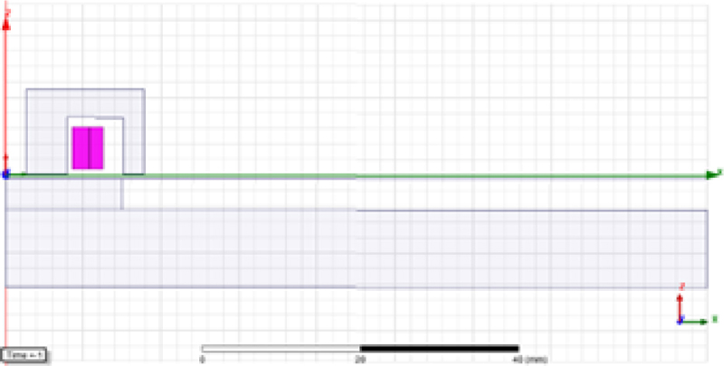
Figure 3: ANSYS Maxwell 2D model.

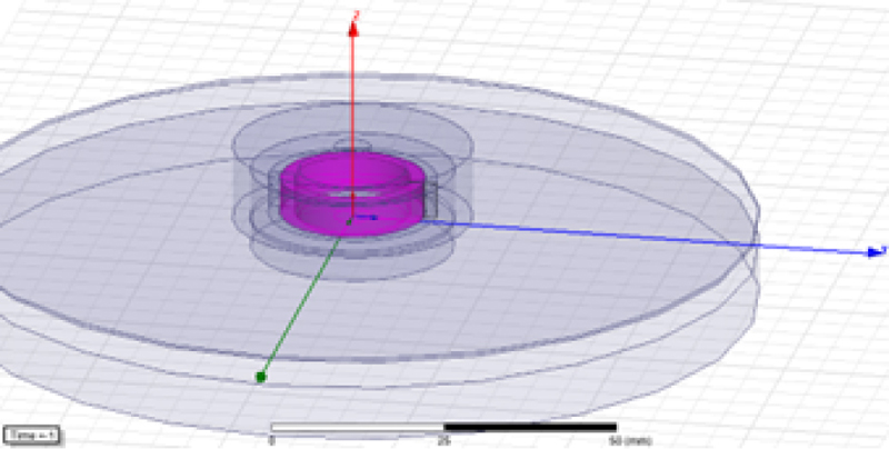
Figure 4: ANSYS Maxwell 3D model.

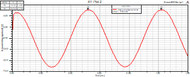
Figure 5: Induced voltage in the pickup coil and the effective value of excitation current and frequency are 0.1 A and 2 kHz, respectively.

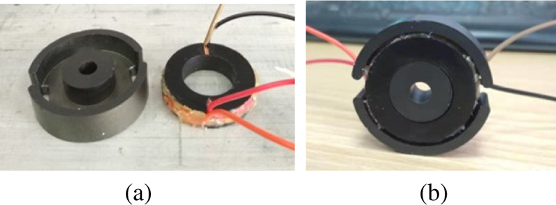
Figure 6: (a) E-core, driver-pickup coils and (b) E-core probe used in experiments.

The correctness of the analytical model is also verified by experimental measurement.

The E-core and homemade driver and pickup coils are shown in Fig. 6. The material characteristic parameters of the magnetic core and conductor are collected from the manufacturers. All parameters used in experiments are shown in Table 1.

The effective value of the sinusoidal excitation current applied to the driver coil is maintained at 0.1 A by adjusting the amplitude of the sinusoidal signal in the signal generator and the amplification factor of the power amplifier. The induced voltage in the pickup coil is measured by a millivolt meter.

Firstly, when the driver coil is excited by a sinusoidal signal with a frequency range from 0.1 kHz to 10 kHz, the induced voltage in the pickup coil of the E-core probe located above a layered conductor is measured. The second layer is a cylindrical conductor with a radius of 15 mm and a thickness of 4 mm, and the other layers are square conductive plates with a side length of 15 cm and different thicknesses. Then, the cylindrical conductor of the second layer is replaced with a non-conductive material of equal thickness, and the above measurement is repeated. Finally, when the layered conductor is absent, the above measurements are repeated again.

Table 1: Parameters of E-core, coils, and conductor used in analytical calculation, FEM and experiment

Coil
Inner radius of driver coil	r${}_{\mathrm{1}}$	8.58 mm
Outer radius of driver coil	r${}_{\mathrm{2}}$	10.7 mm
Inner radius of pickup coil	r${}_{\mathrm{3}}$	10.8 mm
Outer radius of pickup coil	r${}_{\mathrm{4}}$	12.5 mm
Parameter	z${}_{\mathrm{1}}$, z${}_{\mathrm{3}}$	0.74 mm
Parameter	z${}_{\mathrm{2}}$, z${}_{\mathrm{4}}$	6.14 mm
Excitation current	I	0.1 A
Number of turns (driver)	N${}_d$	280
Number of turns (pickup)	N${}_p$	310
Ferrite Core
Inner column radius	a${}_{\mathrm{1}}$	2.7 mm
Outer column radius	a${}_{\mathrm{2}}$	7.95 mm
Inner core radius	a${}_{\mathrm{3}}$	15.1 mm
Outer core radius	a${}_{\mathrm{4}}$	17.74 mm
Core liftoff	h${}_{\mathrm{0}}$	0.1 mm
Inner core height	h${}_{\mathrm{1}}$	7.4 mm
Outer core height	h${}_{\mathrm{2}}$	11.1 mm
Core permeability	$\mu$${}_f$	3500
Conductor
Parameter	d${}_{\mathrm{1}}$	0.5 mm
Parameter	d${}_{\mathrm{2}}$	4.5 mm
Parameter	d${}_{\mathrm{3}}$	5 mm
Cylindrical conductor radius	c	15 mm
Relative permeability	$\mu$${}_6$,$\mu$${}_7$,$\mu$${}_8$,$\mu$${}_9$	1
Conductivity	$\sigma$${}_6$,$\sigma$${}_7$,$\sigma$${}_8$,$\sigma$${}_9$	36 MS/m
Radius of the domain	b	60 mm

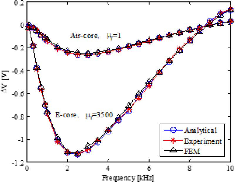
Figure 7: The relationship between excitation frequency and the change of induced voltage in the pickup coil due to cylindrical conductor for an air-core coil ($\mu$${}_f$= 1) and an E-core coil ($\mu$${}_f$= 3500).

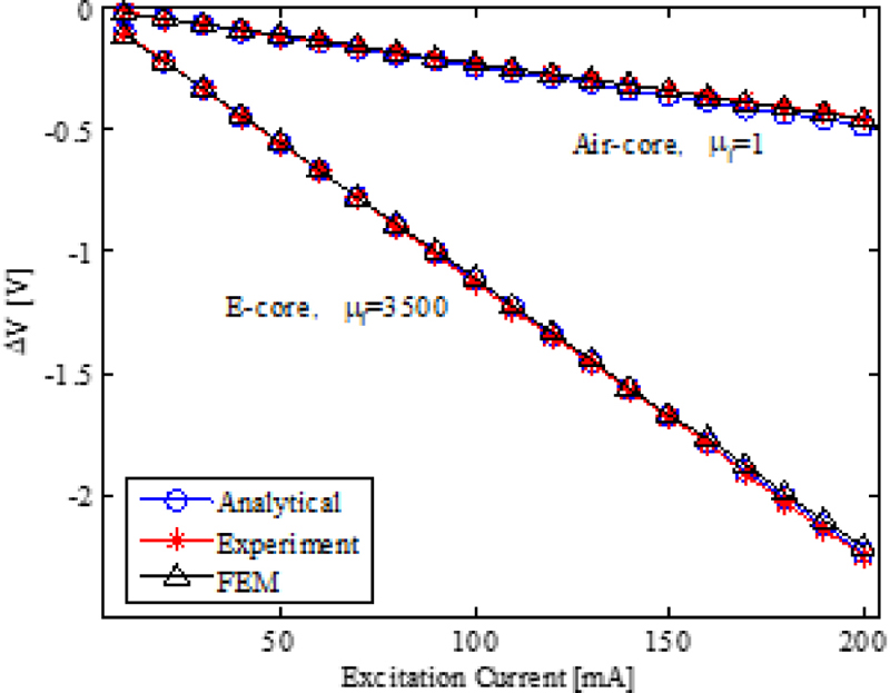
Figure 8: The relationship between the excitation current and the change of induced voltage in the pickup coil due to the cylindrical conductor for an air-core coil ($\mu$${}_f$= 1) and an E-core coil ($\mu$${}_f$= 3500).

V. RESULTS AND DISCUSSION

First, as shown in Fig. 2 (b), equation (20) is used to calculate the induced voltage in the pickup coil when the E-core probe is located above the multilayer conductor. The excitation current is 0.1 A, and the excitation frequency range is 0.1 kHz to 10 kHz. Then the induced voltages in the pickup coil without layered conductor and without hidden cylindrical conductor are calculated, respectively. The calculations are implemented in Mathematica using the parameters shown in Table 1. In all these calculations, the solution domain truncation value b = 60 mm (5 times the outer radius of the outer coil) and the number of summation terms N${}_s$ = 60.

The analytical calculation results are compared with those of FEM and experiment. When the driver coil is excited by current signals of different frequencies, the relationship between the changes of the effective value of the induced voltage in the pickup coil and the excitation frequency due to the hidden cylindrical conductor is shown in Fig. 7. When the excitation frequency is increased, the absolute value of the induced voltage change in the pickup coil first increases and then decreases, and the maximum value of the induced voltage change occurs when the excitation frequency is approximately 2.5 kHz. When the excitation frequency is fixed at 2 kHz and only the excitation current is changed, the change of induced voltage in the pickup coil due to the cylindrical conductor is shown in Fig. 8. The results show that as the excitation current increases, the change of induced voltage in the pickup coil alsoincreases.

In all the above cases, the change of induced voltage in the pickup coil of the E-core probe is larger than that of the air-core probe, which indicates that the E-core probe has a higher sensitivity than that of the air-core probe.

For E-core driver and pickup coils probe, in all cases the relative error of $\mathrm{\Delta }$V between analytical calculation and experimental measurement or FEM is less than 2%, which shows a good agreement.

VI. CONCLUSION

The analytical model of an E-core driver and pickup coils probe over a layered conductor containing hidden cylindrical conductor is proposed using the TREE method. The expressions for the induced voltage in the pickup coil are derived for the general case and for several special cases. The analytical results are compared with the results of experiment and FEM, and they are in good agreement. The proposed analytical model can be used for the design of ferrite cored driver-pickup probes, ECT simulation of multilayer conductors, and can also be used directly for the detection and evaluation of hidden metallic components (such as coins and corrosion) in layered conductive materials.

REFERENCES

[1] S. Zhang, “Analytical model of an I-core coil for nondestructive evaluation of a conducting cylinder below an infinite plane conductor,” Measurement Science Review, vol. 21, no. 4, pp. 99-105, 2021.

[2] T. Theodoulidis and J. R. Bowler, “Impedance of a coil at an arbitrary position and orientation inside a conductive borehole or tube,” IEEE Transactions on Magnetics, vol. 51, no. 4, pp. 1-6, 2015.

[3] T. Theodoulidis and R. J. Ditchburn, “Mutual impedance of cylindrical coils at an arbitrary position and orientation above a planar conductor,” IEEE Transactions on Magnetics, vol. 43, no. 8, pp. 3368-3370, 2007.

[4] D. Desjardins, T. W. Krause, and L. Clapham, “Transient response of a driver-pickup coil probe in transient eddy current testing,” NDT & E International, vol. 75, pp. 8-14, 2015.

[5] H. Huang and T. Takagi, “Inverse analysis for natural and multicracks using signals from a differential transmit-receive ECT probe,” IEEE Transactions on Magnetics, vol. 38, no. 2, pp. 1009-1012, 2002.

[6] S. Zhang and C. Ye, “Model of ferrite-cored driver-pickup coil probe application of TREE method for eddy current nondestructive evaluation,” Applied Computational Electromagnetics Society (ACES) Journal, vol. 37, no. 5, pp. 632-638,2022.

[7] Z. Chen, G. Preda, O. Mihalache, and K. Miya, “Reconstruction of crack shapes from the MFLT signals by using a rapid forward solver and an optimization approach,” IEEE Transactions on Magnetics, vol. 38, no. 2, pp. 1025-1028,2002.

[8] W. Cheng, K. Miya, and Z. Chen, “Reconstruction of cracks with multiple eddy current coils using a database approach,” Journal of Nondestructive Evaluation, vol. 18, no. 4, pp. 149-160,1999.

[9] C. V. Dodd and W. E. Deeds, “Analytical solutions to eddy current probe coil problems,” Journal of Applied Physics, vol. 39, no. 6, pp. 2829-2838, 1968.

[10] T. Theodoulidis and E. E. Kriezis, Eddy Current Canonical Problems (With Applications to Nondestructive Evaluation), Tech Sci. Press, Duluth, Georgia, 2006.

[11] S. Zhang, “An analytical model of a new T-cored coil used for eddy current nondestructive evaluation,” Applied Computational Electromagnetics Society (ACES) Journal, vol. 35, no. 9, pp. 1099-1104, 2020.

[12] G. Tytko and L. Dziczkowski, “E-cored coil with a circular air gap inside the core column used in eddy current testing,” IEEE Transactions on Magnetics, vol. 51, no. 9, pp. 1-4, 2015.

[13] G. Tytko, “An eddy current model of pot-cored coil for testing multilayer conductors with a hole,” Bulletin of the Polish Academy of Sciences Technical Sciences, vol. 68, no. 6, pp. 1311-1317, 2020.

[14] G. Tytko, “Measurement of multilayered conductive discs using eddy current method,” Measurement, vol. 204, pp. 112053, 2022.

[15] S. Zhang, “Analytical model of a T-core coil above a multi-layer conductor with hidden hole using the TREE method for nondestructive evaluation,” COMPEL: The International Journal for Computation and Mathematics in Electrical and Electronic Engineering, vol. 40, no. 6, pp. 1104-1117, 2021.

[16] D. Vasic, D. Ambrus, and V. Bilas, “Computation of the eigenvalues for bounded domain eddy-current models with coupled regions,” IEEE Transactions on Magnetics, vol. 52, no. 6, 7004310, 2016.

[17] G. Tytko and L. Dawidowski, “Locating complex eigenvalues for analytical eddy-current models used to detect flaws,” COMPEL: The International Journal for Computation and Mathematics in Electrical and Electronic Engineering, vol. 38, no. 6, pp. 1800-1809, 2019.

[18] T. Theodoulidis, A. Skarlatos, and G. Tytko, “Computation of eigenvalues and eigenfunctions in the solution of eddy current problems,” Sensors, vol. 23, no. 6, p. 3055, 2023.

APPENDIX

$$\begin{array}{cc}\hfill \mathbf{T}=& {\int }_0^{a_1}r{J}_0(\mathbf{q}r)J_0(\mathbf{m}r)\mathit{d}r+{\int }_{a_1}^{a_4}r{J}_0(\mathbf{q}r)R_0(\mathbf{m}r)\mathit{d}r\hfill \\ & +{\int }_{a_4}^{b}r{J}_0(\mathbf{q}r)R_0^{\prime }(\mathbf{m}r)\mathit{d}r\hfill \end{array},$$

(A.1)

$$\begin{array}{cc}\hfill \mathbf{U}=& {\int }_0^{a_1}r{J}_1(\mathbf{q}r)J_1(\mathbf{m}r)\mathit{d}r+\frac{1}{{\mu }_f}{\int }_{a_1}^{a_4}r{J}_1(\mathbf{q}r)R_1(\mathbf{m}r)\mathit{d}r\hfill \\ & +{\int }_{a_4}^{b}r{J}_1(\mathbf{q}r)R_1(\mathbf{m}r)\mathit{d}r\hfill \end{array},$$

(A.2)

$$\begin{array}{cc}\hfill \mathbf{F}=& {\int }_0^{a_1}r{J}_0(\mathbf{m}r)J_0(\mathbf{m}r)+{\int }_{a_1}^{a_4}r{R}_0(\mathbf{m}r)R_0(\mathbf{m}r)dr)\hfill \\ & +{\int }_{a_4}^{b}r{R}_0^{\prime }(\mathbf{m}r)R_0^{\prime }(\mathbf{m}r)\mathit{d}r\hfill \end{array},$$

(A.3)

$$\begin{array}{cc}\hfill \mathbf{G}=& {\int }_0^{a_1}r{J}_0(\mathbf{m}r)J_0(\mathbf{p}r)\mathit{d}r+{\int }_{a_1}^{a_2}r{R}_0(\mathbf{m}r)L_0(\mathbf{p}r)\mathit{d}r\hfill \\ & +{\int }_{a_2}^{a_3}r{R}_0(\mathbf{m}r)L_0^{\prime }(\mathbf{p}r)\mathit{d}r+{\int }_{a_3}^{a_4}r{R}_0(\mathbf{m}r)L_0^{{}^{\prime \prime }}(\mathbf{p}r)\mathit{d}r\hfill \\ & +{\int }_{a_4}^{b}r{R}_0^{\prime }(\mathbf{m}r)L_0^{{}^{\prime \prime \prime }}(\mathbf{p}r)dr)\hfill \end{array},$$

(A.4)

$$\begin{array}{cc}\hfill \mathbf{H}=& {\int }_0^{a_1}{J}_1\left(\mathbf{m}r\right)J_1\left(\mathbf{p}r\right)\mathit{d}r+\frac{1}{{\mu }_f}{\int }_{a_1}^{a_2}r{R}_1\left(\mathbf{m}r\right)L_1\left(\mathbf{p}r\right)\mathit{d}r\hfill \\ & +{\int }_{a_2}^{a_3}r{R}_1\left(\mathbf{m}r\right)L_1^{\prime }\left(\mathbf{p}r\right)\mathit{d}r+\frac{1}{{\mu }_f}{\int }_{a_3}^{a_4}r{R}_1\left(\mathbf{m}r\right)L_1^{{}^{\prime \prime }}\left(\mathbf{p}r\right)\mathit{d}r\hfill \\ & +{\int }_{a_4}^{b}r{R}_1^{\prime }\left(\mathbf{m}r\right)L_1^{{}^{\prime \prime \prime }}\left(\mathbf{p}r\right)\mathit{d}r\hfill \end{array},$$

(A.5)

$$\begin{array}{cc}\hfill \mathbf{D}=& {\int }_0^{a_1}r{J}_1(\mathbf{p}r)J_1(\mathbf{p}r)\mathit{d}r+\frac{1}{{\mu }_f}{\int }_{a_1}^{a_2}r{L}_1(\mathbf{p}r)L_1(\mathbf{p}r)\hfill \\ & +{\int }_{a_2}^{a_3}r{L}_1^{\prime }(\mathbf{p}r)L_1^{\prime }(\mathbf{p}r)\mathit{d}r+\frac{1}{{\mu }_f}{\int }_{a_3}^{a_4}r{L}_1^{{}^{\prime \prime }}(\mathbf{p}r)L_1^{{}^{\prime \prime }}(\mathbf{p}r)\mathit{d}r\hfill \\ & +{\int }_{a_4}^{b}r{L}_1^{{}^{\prime \prime \prime }}(\mathbf{p}r)L_1^{{}^{\prime \prime \prime }}(\mathbf{p}r)\mathit{d}r\hfill \end{array},$$

(A.6)

$$\begin{array}{cc}\hfill {\mathbf{G}}^{*}=& {\int }_0^{a_1}r{J}_0(\mathbf{p}r)J_0(\mathbf{q}r)+{\int }_{a_1}^{a_2}r{L}_0(\mathbf{p}r)J_0(\mathbf{q}r)\mathit{d}r\hfill \\ & +{\int }_{a_2}^{a_3}r{L}_0^{\prime }(\mathbf{p}r)J_0(\mathbf{q}r)\mathit{d}r+{\int }_{a_3}^{a_4}r{L}_0^{{}^{\prime \prime }}(\mathbf{p}r)J_0(\mathbf{q}r)\hfill \\ & +{\int }_{a_4}^{b}r{L}_0^{{}^{\prime \prime \prime }}(\mathbf{p}r)J_0(\mathbf{q}r)\mathit{d}r\hfill \end{array},$$

(A.7)

$$\begin{array}{cc}\hfill {\mathbf{H}}^{*}=& {\int }_0^{a_1}r{J}_1(\mathbf{p}r)J_1(\mathbf{q}r)+{\int }_{a_1}^{a_2}r{L}_1(\mathbf{p}r)J_1(\mathbf{q}r)\mathit{d}r\hfill \\ & +{\int }_{a_2}^{a_3}r{L}_1^{\prime }(\mathbf{p}r)J_1(\mathbf{q}r)\mathit{d}r+{\int }_{a_3}^{a_4}r{L}_1^{{}^{\prime \prime }}(\mathbf{p}r)J_1(\mathbf{q}r)\hfill \\ & +{\int }_{a_4}^{b}r{L}_1^{{}^{\prime \prime \prime }}(\mathbf{p}r)J_1(\mathbf{q}r)\mathit{d}r\hfill \end{array},$$

(A.8)

$$\begin{array}{cc}\hfill \mathbf{N}=& {\mathbf{vu}}^{-1}{\mathbf{F}}_1(\mathbf{u}c){\int }_0^{c}r{J}_0(\mathbf{q}r)J_0(\mathbf{v}r)\mathit{d}r\hfill \\ & +J_1(\mathbf{v}c){\int }_c^{b}r{J}_0(\mathbf{q}r){\mathbf{F}}_0(\mathbf{u}r)\mathit{d}r\hfill \end{array},$$

(A.9)

$$\begin{array}{cc}\hfill \mathbf{N}*=& F_1(\mathbf{u}c){\int }_0^{c}r{J}_1(\mathbf{q}r)J_1(\mathbf{v}r)\mathit{d}r\hfill \\ & +J_1(\mathbf{v}c){\int }_c^{b}r{J}_1(\mathbf{q}r)F_1(\mathbf{u}r)\mathit{d}r\hfill \end{array}.$$

(A.10)

BIOGRAPHIES

Siquan Zhang received the Ph.D. degree in material processing engineering from the South China University of Technology, Guangzhou, China. His current research interests include eddy current testing and analytical models in non-destructive testing.

ACES JOURNAL, Vol. 38, No. 11, 914–921
doi: 10.13052/2023.ACES.J.381110
© 2023 River Publishers

ABSTRACT

I. INTRODUCTION

II. SOLUTION

III. SPECIAL CASES

IV. FEM AND EXPERIMENT VALIDATION

V. RESULTS AND DISCUSSION

VI. CONCLUSION

REFERENCES

APPENDIX

BIOGRAPHIES