Performance Comparison Between Fingerprinting-based RSS Indoor Localization Techniques at WLAN Frequencies: Simulation Study

Huthaifa Obeidat $^{1}$ , Eyad Alzuraiqi $^{2}$ , Issam Trrad $^{1}$ , Nouh Alhindawi $^{3,4}$ , and Mohammad R. Rawashdeh $^{2}$

¹Faculty of Engineering
Jadara University, Irbid, Jordan
h.obeidat@jadara.edu.jo, itrrad@jadara.edu.jo

²Hijjawi Faculty for Engineering Technology
Yarmouk University, Irbid, Jordan
eyad.zuraiqi@yu.edu.jo, alrwashd@yu.edu.jo

³Faculty of Sciences and Information
Jadara University, Irbid, Jordan
hindawi@jadara.edu.jo

⁴Ira A. Fulton Schools of Engineering, School of Computing and Augmenting Intelligence (SCAI)
Arizona State University, Arizona, USA
nalhinda@asu.edu

Submitted On: September 11, 2024; Accepted On: December 3, 2024

ABSTRACT

This paper presents a performance comparison between two fingerprinting-based received signal strength (RSS) indoor localization techniques at wireless local-area network (WLAN) frequencies: 2.4 GHz and 5.8 GHz. The investigated algorithms include the comparative RSS (CRSS) and vector algorithms. The study was conducted using Wireless InSite ray-tracer software. The simulation was conducted in a simulated environment on the 3rd floor of the Chesham Building, University of Bradford, UK. Also, we presented an estimator which looks at the correlation between the test point RSS and the reference point RSS. The estimator performance is compared to the root mean square error (RMSE) performance. It was found that the CRSS algorithm suffers from the similarity problem while constructing the radio map, and it also suffers from ambiguity problems during localization. The vector algorithm outperforms CRSS algorithms in both frequencies and does not suffer from similarity or ambiguity problems. The proposed estimator shows better performance at both frequencies.

Index Terms: Indoor localization, received signal strength (RSS), Wireless InSite, wireless local-area network (WLAN).

I. INTRODUCTION

Localization has become essential for pervasive applications, including medical healthcare, behavior recognition, and smart buildings [1]. Localization in outdoor environments has been resolved thanks to global navigation satellite systems (GNSS), such as the global positioning system (GPS), the European GALILEO, the Russian GLONASS, and the Chinese BeiDou Satellite Navigation System. Using GNSS, the customer can infer the whereabouts of his location by using received satellite signals from his smartphone. Unfortunately, the GNSS signal cannot penetrate through buildings; therefore, the demand to localize people and items inside indoor environments encouraged researchers to utilize other technologies for localization, including Wi-Fi [2], satellite [3], inertial [4], magnetic [5], ultrasound [6], infrared [7], frequency modulation (FM) waves [8], ZigBee [9], Bluetooth [10], ultra-wideband (UWB) [11], and radio-frequency identification (RFID) [12].

In [13], the authors summarized the usage percentage of localization techniques in indoor environments, as seen in Table 1. RF-based techniques are widely used in indoor environments, representing 73% of all adopted indoor localization techniques. Wi-Fi is the most used technology within the RF-based techniques category, followed by Bluetooth. Hybrid technologies were introduced to enhance accuracy. Table 2 presents the pros and cons of using RF technologies in localization within indoor environments.

Table 1: Usage percentage of localization technologies in indoor environments

Localization Technique	Usage Percentage
Infrared	9%
Ultrasound	6%
GPS	4%
Magnetic	1%
Vision	1%
Other	6%
RF Positioning	Wi-Fi	24%	73%
Bluetooth	17%
RFID	7%
Ultra-Wideband	6%
UHF	4%
Cellular	1%
Hybrid	6%
Cooperative Sensor-Based	8%

Table 2: Advantages and disadvantages of RF technologies used in indoor localization

Technology	Advantage	Disadvantage
Wi-Fi	Low costWidely deployed	Requires training
Bluetooth	Low costSmartphones can collect signals	Requsirestraining
RFID	Low costHigh accuracy	Deployment is tiresomeCoverage area is small
Ultra-Wideband	High accuracy	ExpensiveRequires special equipment
mm-wavetechnology	Massivebandwidth High accuracy	Huge penetration losses
Cellular	Low cost	Low accuracy

Wi-Fi technology is widely used globally since the infrastructure is implanted in most commercial, industrial, educational, and residential facilities [14]. Additionally, smartphones can be used as receivers, which makes the technology cheap. The main challenge for localization using Wi-Fi technology is to reach the cm-level accuracy. Within the Wi-Fi data, many signal measures can be used for localization, RSS, channel state information (CSI) and round trip time (RTT), time of arrival, and angle of arrival [14].

RSS is the most popular measure. The data are collected from the surrounding access points (APs) at each location. If the RSS is less than the receiver sensitivity, the signal is said to be undetected [15]. Triangulation and fingerprinting techniques use RSS data for localization [16, 17]. RSS is sensitive to the effect of superimposition of multipath signals of different phases; therefore, by taking the mean value of the locally close RSS values, the effect of fast fading is reduced [18].

By averaging over access points with multiple frequencies and/or heights, the variation of recorded RSS becomes less. The less variation, the more monotonic relationship between distance from access point and recorded RSS; therefore, localization error becomes less [19].

Channel properties of a communication link, also known as CSI, can be used for Wi-Fi localization, discriminating multipath, and increasing localization accuracy. Compared to RSS, the CSI is more stable [20]. However, Wi-Fi network interference cards are needed [21]. RTT is distinguished from time of arrival (TOA) and time difference of arrival (TDOA) as it does not require clock synchronization between the transmitter and receiver [22]. The transmitter sends a message to the receiver and records the timestamp, the receiver sends back an acknowledgment, and then the transmitter estimates the RTT. However, both transmitter and receiver have error measurements due to processing time and phase noise [23].

The TOA method measures travel time between the AP and the receiver. The distance is calculated by multiplying the TOA by the speed of light, and both the transmitter and receiver must be synchronized [24]. For 2D localization, 3 APs are required to perform trilateration. For 3D scenarios, 4 APs are needed. This technique requires larger bandwidth (BW). For example, using a 10 MHz BW, the time resolution will be 10 $^{- 7}$ s, and the error will be up to 30 m. However, using a 1 GHz BW, the time resolution will be 10 $^{- 9}$ s, and the error will be reduced to about 0.03 m. Therefore, it is widely used with UWB positioning technologies [25]. The enormous BW available in the 5G and 6G networks will make the utilization of TOA in localization more realizable [26, 27].

The angle of arrival (AOA) can be calculated by estimating the phase differences on the antenna elements. Estimation using AOA requires 2 APs for 2D localization and 3 APs for 3D localization. However, the cost is relatively high compared to other techniques. Additionally, AOA techniques suffer from multipath and low signal-to-noise ratios [28]. In [29], authors proposed a hybrid technique that combines TOA and AOA. This reduced the number of APs needed, the system required large BW, and it leverages the benefits from both techniques.

In this paper, we compared the localization performance of two radio-frequency algorithms at the wireless local-area network (WLAN) frequencies. The investigated algorithms are fingerprinting-based algorithms, including the comparative received signal strength (CRSS) algorithm and the vector algorithm. This work is an extension of the work done in [30]; however, we adopted different frequencies.

Also, we proposed an estimator that considers the correlation between the test point (TP) RSS and the reference point (RP) RSS while estimating the closest RP to the TP. The estimator checks the similarity between the RSS received at a TP from an AP and other RSS values collected at all RPs from the same AP. This process is for all APs in the facility. By taking the summation of likenesses, the closest RP to the TP will be the one with maximum likeness. The order of this paper is as follows. Section II investigates the examined algorithms. Section III presents the methodology and simulation setup, section IV discusses the results, and conclusions are drawn in section V.

II. INVESTIGATED ALGORITHMS

The proposed algorithms are radio-frequency fingerprinting-based algorithms, where data are collected from known locations. A radio map is constructed by mapping the received signal strength (RSS) data collected from each receiver point to its location. This stage is known as the offline phase. In the next stage (the online phase), RSS data are collected from unknown locations termed TP and, by using the radio map, the TP data are compared to the radio-map database. The RP with the lowest RSS difference is assumed to be the closest RP.

In this study, we compared two algorithms. The first algorithm is the vector algorithm [31], where data collected are stored in vectors, and each vector represents the RSS collected at the RP from the surrounding APs. TP data are also stored as a vector. The TP vector is compared to each vector in the radio map by estimating the root mean square error (RMSE) between the TP-RSS vector and each RP-RSS vector in the radio map. The RP whose vector achieves the lowest RMSE is said to be the closest location to the TP. The RMSE between the RSS values of the j $^{t h}$ RP and the TP isgiven by:

e_{j} = \sqrt{\frac{\sum_{i = 1}^{N} {(c_{i j} - t_{i})}^{2}}{N}},

(1)

where N is the number of the APs, $t_{i}$ is the RSS collected at TP from the i $^{t h}$ AP, and c $_{i j}$ is the RSS collected by the j $^{t h}$ RP from the i $^{t h}$ AP.

RMSE is a popular metric since it is understandable by showing the average error in the same units as the data. It highlights larger errors, which is beneficial for avoiding big errors. RMSE is widely used as it provides a comprehensive measure of accuracy by combining the average and variability of errors, making it easy to compare results across different studies and models [32].

Another popular estimator is the mean average error (MAE). The MAE is easy to understand, robust to outliers, and it performs well even when the target variable has skewed distributions. The MAE between the RSS values of the k $^{t h}$ RP and the TP is given by:

e e_{k} = \frac{1}{N} \sum_{i = 1}^{N} | c_{i k} - t_{i} | .

(2)

We introduced another estimator, which sees how similar the RSS collected at a TP is from an AP to other RSS values collected at all RPs from the same AP. The likeness percentage (LP) is estimated by:

l_{i} = 1 - | \frac{c_{i j} - t_{i}}{c_{i j}} | .

(3)

When l equals 1, both TP and RP record the same RSS from an AP; the more l approaches one, the more the likeness between TP and RP. For all APs in the facility, the summation of likenesses is taken as shown in (4); the closest RP to the TP will be the one with maximum likeness:

L = \sum_{i = 1}^{N} l_{i} = \sum_{i = 1}^{N} 1 - | \frac{c_{i j} - t_{i}}{c_{i j}} | .

(4)

Using different estimators in localization is common, as in [33], where authors proposed using Spearman distance instead of Euclidean distance. The simulation results show improved results. The LP estimator searches for similarity instead of difference. Rather than exaggerating the effect of enormous errors, the error levels are equally treated.

The second algorithm is the CRSS, where at each RP/TP RSS vector, the algorithm compares each RSS value of the vector with the other values collected in the same vector. The comparison was made based on the following equation [34]:

	$M_{N}$	$= [c_{i k}] i, k = 1, 2, \dots, N,$		(5)
	$c_{i k}$	$= {\begin{matrix} \binom{+ 1 R_{i} > R_{k} > R_{s e n s}}{- 1 R_{k} > R_{i} > R_{s e n s}} \\ \binom{0 R_{i} = R_{k} > R_{s e n s}}{+ 2 R_{i} > R_{s e n s} > R_{k}} \\ \binom{- 2 R_{k} > R_{s e n s} > R_{i}}{+ 3 R_{s e n s} > [R_{k}, R_{i}]} \end{matrix},$		(6)

where $M_{N}$ is the constructed matrix, $R_{i}$ is the RSS value to be compared to other RSS values $R_{k}$ , and $R_{s e n s}$ is the receiver sensitivity. Both i and k range from 1 to N. For example, if the RSS vector was v $=$ [ $-$ 59.59 $-$ 34.1 $-$ 59.02 $-$ 100 $-$ 95], then the generated CRSS matrix is given as:

CRSS = [\begin{matrix} \begin{matrix} 0 & \begin{matrix} - 1 & - 1 \end{matrix} & + \begin{matrix} 2 & + 2 \end{matrix} \end{matrix} \\ + \begin{matrix} 1 & \begin{matrix} 0 & + 1 \end{matrix} & + \begin{matrix} 2 & + 2 \end{matrix} \end{matrix} \\ \begin{matrix} + 1 & \begin{matrix} - 1 & 0 \end{matrix} & \begin{matrix} + 2 & + 2 \end{matrix} \end{matrix} \\ \begin{matrix} - 2 & \begin{matrix} - 2 & - 2 \end{matrix} & \begin{matrix} 0 & + 3 \end{matrix} \end{matrix} \\ \begin{matrix} - 2 & \begin{matrix} - 2 & - 2 \end{matrix} & \begin{matrix} + 3 & 0 \end{matrix} \end{matrix} \end{matrix}] .

(7)

This process is accomplished for every RSS vector in the radio map; the resultant matrices are saved as a new radio map. During localization, the RSS of the TP-RSS vector is converted into a CRSS matrix and then compared to the new radio map. The closest location is the RP, with the lowest RMSE between its corresponding CRSS matrix and the TP-CRSS matrix.

Fingerprinting localization is one of the most common techniques. The investigated algorithms include the CRSS algorithm and the vector algorithm. In a previous paper, the performance between the two algorithms is tested at a lower frequency of 400 MHz [30]; in this paper, the performance is examined at microwave frequencies 2.4 and 5.8 GHz. The target of this study is to examine the robustness of the CRSS algorithm at microwave frequencies.

III. METHODOLOGY AND SIMULATION SETUP

The simulations were done using Wireless InSite® (WI) ray-tracing software, which has been validated over WLAN frequencies [35, 36]. In this project, a detailed layout of the 3rd floor of the Chesham Building at the University of Bradford was constructed; the design took into account the materials of the building, including concrete, drywall, glass, and wood.

WI allows modeling the floor as seen in Fig. 1, where the user can change the electrical constitutive parameters (permittivity and conductivity). The user can set up the communication links between transmitters and receivers. This includes the type of antenna used, transmitted power, operating frequency, signal BW, the maximum number of reflections, transmissions, and diffractions, propagation model, ray-tracing method, sum complex electric fields, and the number of propagation paths.

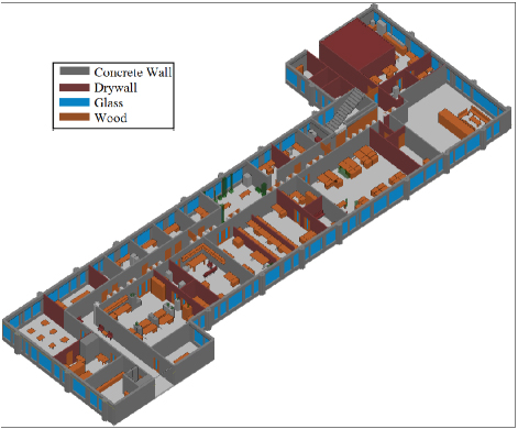
Figure 1: Simulated environment for the 3rd floor in the Chesham Building, University of Bradford, UK.

Adding more paths, transmissions, reflections, and diffractions will be at the expense of computational time. Sufficient results were found when the maximum number of paths is 10, the number of transmissions is 4, and the number of reflections is 4 [35]. Table 3 summarizes the settings used in the WI software for both operating frequencies: 2.4 GHz and 5.8 GHz. Table 4 presents the permittivity $ε$ $_{r}$ and conductivity $σ$ values used in our simulations based on the ITU tables [37]. The permittivitydoes not change considerably with frequency contradictory to the conductivity.

Table 3: Wireless InSite settings for the investigatedscenario

Setting	Value
Transmitter antenna	3-element somni directional array
Antenna gain	3.5 (2.4 GHz)4.5 (5.8 GHz)
Receiver antenna	Omnidirectional
Sum complexelectric fields	None
Operating frequency	2.4 GHz5.8 GHz
Bandwidth	20 MHz (2.4 GHz)40 MHz (5.8 GHz)
Number of reflections	4
Number of transmissions	4
Number of diffractions	0
Ray-spacing	0.1 $^{\circ}$
Plane-wave ray spacing	0.5 m
Maximumrendered paths	10
Ray-tracing method	Shooting-and-Bouncing-Rays (SBR)
Ray-tracing acceleration	Octree
Propagation model	full 3D

Table 4: Material properties with frequency

Material	2.4 GHz	5.8 GHz
	$ε_{r}$	$σ$	$ε_{r}$	$σ$
Concrete	5.31	0.0662	5.31	0.1258
Glass	6.27	0.0122	6.27	0.0314
Wood	1.99	0.0120	1.99	0.0281
Drywall	2.94	0.0216	2.94	0.0378

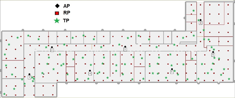
Figure 2: APs, RPs, and TPs distribution on the 3rd floor of the Chesham Building.

As mentioned earlier, the localization techniques used in this article are RF-fingerprinting-based algorithms. Figure 2 shows the distribution of the APs, RPs, and TPs. There are 7 APs, 176 RPs, and 85 TPs. The choice of these numbers was based on recommendations from a previous study [30]. In that paper, the effect of adding more APs and RP is examined. It was found that adding more APs will enhance the localization performance; however, the vector and matrix sizes will be larger. Adding more RPs will enhance the performance up to a certain limit; after that, adding more RPs will not enhance the performance, it may worsen it.

Based on the above, the number of APs and RPs was set to ensure the best performance. Our paper uses 7 APs to ensure that at least 4 APs cover all regions within the floor. We tried to avoid adding redundant RPs; therefore, the RPs were chosen to have space bigger than 10 $λ$ . This number is used widely to perform averaging to minimize the fast-fading effect; the window could be up to 22 $λ$ . Therefore, the spacing between the RPs will ensure no redundant RPs and, in a practical scenario, the averaging window extends from 10 $λ$ to 22 $λ$ [19].

In Wireless InSite, the fast fading effect is removed by taking the power sum of incident rays rather than considering the phase [38]. The collected data is given to Matlab code; the code builds up the radio map based on the RPs data, and then each TP data is compared to the radio map by estimating the RMSE, MAE, and LP estimators (equations (1)–(3)). The closest RP is estimated when its corresponding RMSE/MAE value is the least or its corresponding LP value is the maximum. The code also generates the CRSS matrices based on equation (5) and builds up the CRSS radio map. Similarly, the code estimates the closest RP by finding the lowest RMSE/MAE.

IV. RESULTS AND DISCUSSION

Using two RF fingerprinting techniques, we have examined localization accuracy for two algorithms at the two WLAN bands: 2.4 GHz and 5.8 GHz.

A. CRSS algorithm

During the generation of the CRSS matrices, it was observed that many RPs are relatively close to each other and construct the same matrix since the descending (or ascending) order of the APs based on their corresponding RSS level is the same for these RPs. As seen in Fig. 3, each contoured set of RPs indicates that the RPs within the contour generate the same CRSS matrix. We refer to this problem as similarity. In this figure, each black contour surrounds RPs that generate the same CRSS. We found that some RPs generate the same CRSS matrix but are not co-located. Therefore, we used different colors for their contours; for example, there are two purple contours on the right-lower side of Fig. 3, meaning these 4 RPs generate the same CRSS matrix.

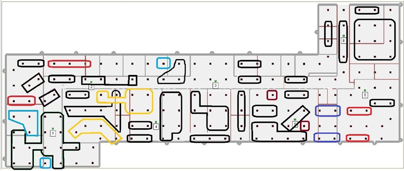
Figure 3: RPs similarity observed at 5.8 GHz. Table 5 shows how many sets of RPs generate the same CRSS matrix. For example, at 5.8 GHz, we found that the number of cases where 2 RPs generate the same CRSS matrix is 17 cases. Similarly, we found that the number of cases where 3 RPs generate the same CRSS matrix is 5. We also found that 13 RPs generate the same CRSS matrix. Similarity tends to worsen as frequency increases. At 2.4 GHz, only 56 RPs out of 176 generated unique CRSS matrices, which comprise 32.3% of the entire RPs set; however, at 5.8 GHz, only 44 RPs generate unique CRSS matrices, which are 25%. We found that only 33 RPs are free from similarity at both frequencies. The figure shows that similarity occurs more in halls and rooms separated by drywalls. However, they tend to be less in rooms separated by concrete walls. This explains why RPs in the upper half of the figure have less similarity. Therefore, using the CRSS algorithm, lower-resolution radio maps are better since having a high-resolution radio map will lead to similarity. A similar observation was recorded at 2.4 GHz.

When localization was conducted at 2.4 GHz, only 20% of TPs were linked to a single RP. For each TP of the remaining 80%, the estimated location is a group of RPs with the same CRSS matrix or different CRSS matrices. At 5.8 GHz, only 23% of TPs were linked to a single RP. As shown in Fig. 4, the estimated TP is linked to RPs with different CRSS matrices.

Table 5: Total of how many sets of RPs generate the same CRSS matrices

Similarity RPs	2.4 GHz	5.8 GHz
	No. of Cases	No. of Cases
2 RPs generate the same matrix	14	17
3 RPs generate the same matrix	9	6
4 RPs generate the same matrix	3	2
5 RPs generate the same matrix	0	2
6 RPs generate the same matrix	2	4
7 RPs generate the same matrix	3	1
8 RPs generate the same matrix	1	0
9 RPs generate the same matrix	0	2
10 RPs generate the same matrix	1	0
11 RPs generate the same matrix	0	0
12 RPs generate the same matrix	0	0
13 RPs generate the same matrix	0	1
Similarity	67.7%	75%

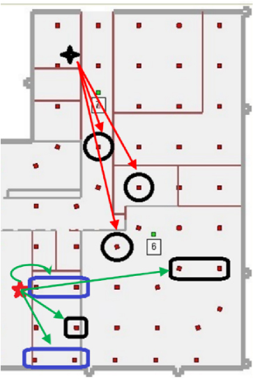
Figure 4: Example of ambiguity at 5.8 GHz.

As seen, the TP (represented by a black tetragram) is linked to 3 RPs, each with a different CRSS matrix; once localization is performed, these RPs are considered the closest. Also, the TP represented by a red star is linked to 7 RPs, which are represented by 3 CRSS matrices (4 of them are represented by a single CRSS, and the RPs contour color is blue). So, in addition to the similarity problem, we have ambiguity problem, when TP location is linked to different RPs which have different CRSS matrices.

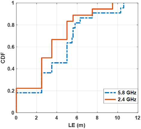
Figure 5: LE comparison using the CRSS algorithm without the ambiguous cases at the WLAN frequencies.

This makes using the CRSS algorithm inefficient; therefore, we do not recommend using this algorithm for localization purposes.

Figure 5 shows a localization error (LE) comparison at the two WLAN frequencies using the CRSS algorithm without considering the ambiguous cases. LE tends to be less at 2.4 GHz when no ambiguity is considered. This means that the accuracy of the CRSS algorithm becomes lower as frequency increases. Also, the similarity effect becomes more significant as frequency increases, as shown in Table 5.

B. Vector algorithm

We have used three estimators: RMSE, MAE, and the proposed LP estimator. Figure 6 shows an LE comparison for each estimator at the two WLAN frequencies. Both RMSE and LP estimators show that localization accuracy decreases as frequency increases; however, MAE shows better performance as frequency increases. For example, using the LP estimator, the probability of localization error less than 2.5 m is 75% and 60% at 2.4 GHz and 5.8 GHz, respectively. Using MAE, the probability for localization error less than 2.5 m is 60% and 50% at 2.4 GHz and 5.8 GHz, respectively. Using RMSE, the probability for localization error less than 2.5 m is 35% and 25% at 2.4 GHz and 5.8 GHz, respectively.

The probability of localization error less than 5 m and 5.5 m is 90% using the LP estimator at 2.4 GHz and 5.8 GHz. Also, 90% of errors are less than 5.5 m and 6 m using the MAE and RMSE estimators at 2.4 GHz and 5.8 GHz, respectively.

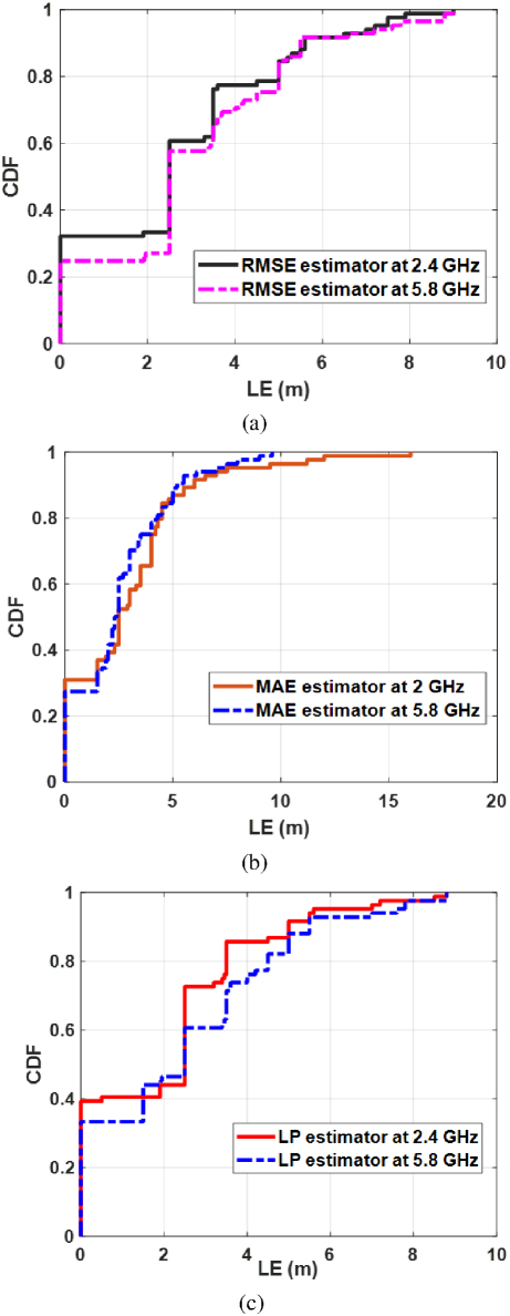
Figure 6: LE comparison for (a) RMSE estimator, (b) MAE estimator, and (c) LP estimator at the two WLAN frequencies.

Results show that the LP estimator tends to show better performance, as shown in Fig. 7. The LP estimator shows better all-over performance at the two WLAN frequencies; for example, at 2.4 GHz, the probability for localization error less than 3.5 m is 86%, 66%, and 76% using LP estimator, MAE estimator, and RMSE estimator, respectively. At 5.8 GHz, the probability of an error being less than 3.5 m is 71%, 75%, and 66% using the LP, MAE, and RMSE estimators, respectively.

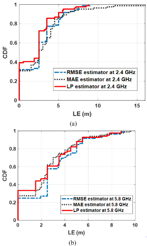
Figure 7: LE comparison between the three estimators at (a) 2.4 GHz and (b) 5.8 GHz.

Tables 6 and 7 present a comparison between the three estimators at the two frequencies. The tables show how many estimated RP were the closest to the TP (the accurate), the second closest RP, and the third closest RP. For example, using the LP estimator at 2.4 GHz, for 33 TPs, the estimated location for each TP was the actual closest RP to that TP. For 27 TPs, the estimated location for each TP was the first neighbor to the closest RP. For 12 TPs, the estimated location for each TP was the second neighbor to the closest RP. The tables show that the LP estimator outperforms the MAE and RMSE estimators at the two WLAN frequencies, as provided by the metrics. It can be seen from the figures and the tables that the best estimator is the LP estimator, followed by the MAE estimator. RMSE squares the errors before averaging, giving more weight to larger errors; therefore, it performs less well.

Table 6: Performance comparison between LP, MAE, and RMSE estimators at 2.4 GHz

	2.4 GHz
	RMSE	MAE	LP
Accurate RP	27	29	33
1st neighbor	24	14	27
2nd neighbor	15	11	12

Table 7: Performance comparison between LP, MAE, and RMSE estimators at 5.8 GHz

	5.8 GHz
	RMSE	MAE	LP
Accurate RP	20	23	28
1st neighbor	28	9	21
2nd neighbor	15	10	17

Figure 8 compares vector and CRSS algorithms when we excluded ambiguity cases at 5.8 GHz. Even when we considered only the cases when the CRSS algorithm detects 1 RP, the vector algorithm performs better. For example, 90% of errors are less than 5.5 m using the vector algorithm, while 90% of errors are less than 7.5 m using the CRSS algorithm.

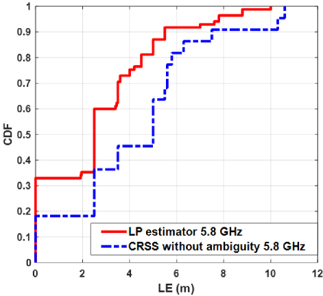
Figure 8: LE comparison between vector and CRSS algorithms when we excluded the ambiguity cases.

V. CONCLUSION

A comparison between two radio-frequency localization techniques at WLAN bands is presented. The algorithms include vector and CRSS algorithms, which are fingerprinting-based RSS techniques. The study was performed in a simulated environment on the 3rd floor of the Chesham Building, University of Bradford, UK, using Wireless InSite software. It was found that the CRSS algorithm suffers from similarity and ambiguity problems; both get worse as frequency increases. Therefore, the algorithm is not recommended for indoor positioning. The vector algorithm shows acceptable performance at both frequencies as the probability for an error to be less than 2.5 m is 72.5% at 2.4 GHz and 60% at 5.8 GHz.

Additionally, the performance of the vector algorithm outperforms the CRSS algorithms, even when we do not consider the ambiguity cases. Also, we introduced a new estimator to find which RP is the closest to the TP based on their RSS values; the estimator considers/utilizes the correlation between the RSS collected by the TP and the RSS collected by the RPs. The performance was compared to MAE and RMSE, showing better performance at bothfrequencies.

REFERENCES

[1] S. Subedi and J.-Y. Pyun, “A survey of smartphone-based indoor positioning system using RF-based wireless technologies,” Sensors, vol. 20, no. 24, p. 7230, 2020.

[2] V. Bellavista-Parent, J. Torres-Sospedra, and A. Perez-Navarro, “New trends in indoor positioning based on Wi-Fi and machine learning: A systematic review,” arXiv Prepr. arXiv2107.14356,2021.

[3] X. Wan and X. Zhan, “The research of indoor navigation system using pseudolites,” Procedia Eng., vol. 15, pp. 1446-1450, 2011.

[4] Z. Chen, Q. Zhu, and Y. C. Soh, “Smartphone inertial sensor-based indoor localization and tracking with iBeacon corrections,” IEEE Trans. Ind. Informatics, vol. 12, no. 4, pp. 1540-1549,2016.

[5] P. Davidson and R. Piché, “A survey of selected indoor positioning methods for smartphones,” IEEE Commun. Surv. Tutorials, vol. 19, no. 2, pp. 1347-1370, 2016.

[6] F. Sainjeon, S. Gaboury, and B. Bouchard, “Real-time indoor localization in smart homes using ultrasound technology,” in Proceedings of the 9th ACM International Conference on Pervasive Technologies Related to Assistive Environments, pp. 1-4, 2016.

[7] B. Mukhopadhyay, S. Sarangi, S. Srirangarajan, and S. Kar, “Indoor localization using analog output of pyroelectric infrared sensors,” in 2018 IEEE Wireless Communications and Networking Conference (WCNC), IEEE, pp. 1-6, 2018.

[8] A. Popleteev, V. Osmani, and O. Mayora, “Investigation of indoor localization with ambient FM radio stations,” in 2012 IEEE International Conference on Pervasive Computing and Communications, IEEE, pp. 171-179, 2012.

[9] A. Billa, I. Shayea, A. Alhammadi, Q. Abdullah, and M. Roslee, “An overview of indoor localization technologies: Toward IoT navigation services,” in 2020 IEEE 5th International Symposium on Telecommunication Technologies (ISTT), IEEE, pp. 76-81, 2020.

[10] R. Giuliano, G. Cardarilli, C. Cesarini, L. Di Nunzio, F. Fallucchi, R. Fazzolari, F. Mazzenga, M. Re, and A. Vizzarri, “Indoor localization system based on Bluetooth low energy for museum applications,” Electronics, vol. 9, p. 1055, 2020.

[11] A. Poulose and D. S. Han, “UWB indoor localization using deep learning LSTM networks,” Appl. Sci., vol. 10, no. 18, p. 6290, 2020.

[12] W. Shuaieb, G. Oguntala, A. AlAbdullah, H. Obeidat, R. Asif, R. Abd-Alhameed, M. Bin-Melha, and C. Kara-Zaïtri, “RFID RSS fingerprinting system for wearable human activity recognition,” Future Internet, vol. 12, p. 33, 2020.

[13] C. Esposito and M. Ficco, “Deployment of RSS-based indoor positioning systems,” Int. J. Wirel. Inf. Networks, vol. 18, no. 4, pp. 224-242, 2011.

[14] X. Feng, K. A. Nguyen, and Z. Luo, “A survey of deep learning approaches for WiFi-based indoor positioning,” J. Inf. Telecommun., pp. 1-54, 2021.

[15] H. Obeidat, W. Shuaieb, O. Obeidat, and R. Abd-Alhameed, “A review of indoor localization techniques and wireless technologies,” Wirel. Pers. Commun., pp. 1-39, 2021.

[16] Y. Wang, X. Yang, Y. Zhao, Y. Liu, and L. Cuthbert, “Bluetooth positioning using RSSI and triangulation methods,” in 2013 IEEE 10th Consumer Communications and Networking Conference (CCNC), IEEE, pp. 837-842, 2013.

[17] H. A. Obeidat, W. Shuaieb, H. Alhassan, K. Samarah, M. Abousitta, R. A. Abd-Alhameed, S. M. R. Jones, and J. M. Noras, “Location based services using received signal strength algorithms,” in 2015 Internet Technologies and Applications (ITA), IEEE, pp. 411-413, 2015.

[18] H. Obeidat, A. A. S. Alabdullah, N. T. Ali, R. Asif, O. Obeidat, M. S. A. Bin-Melha, W. Shuaieb, R. A. Abd-Alhameed, and P. Excell, “Local average signal strength estimation for indoor multipath propagation,” IEEE Access, vol. 7, pp. 75166-75176, 2019.

[19] H. Obeidat, M. Al-Sadoon, C. Zebiri, O. Obeidat, I. Elfergani, and R. Abd-Alhameed, “Reduction of the received signal strength variation with distance using averaging over multiple heights and frequencies,” Telecommun. Syst., vol. 86, no. 1, pp. 201-211, 2024.

[20] X. Zhu, W. Qu, T. Qiu, L. Zhao, M. Atiquzzaman, and D. O. Wu, “Indoor intelligent fingerprint-based localization: Principles, approaches and challenges,” IEEE Commun. Surv. Tutorials, vol. 22, no. 4, pp. 2634-2657, 2020.

[21] M. Li, Y. Meng, J. Liu, H. Zhu, X. Liang, Y. Liu, and N. Ruan, “When CSI meets public Wi-Fi: Inferring your mobile phone password via Wi-Fi signals,” in Proceedings of the 2016 ACM SIGSAC Conference on Computer and Communications Security, pp. 1068-1079,2016.

[22] G. Guo, R. Chen, F. Ye, X. Peng, Z. Liu, and Y. Pan, “Indoor smartphone localization: A hybrid Wi-Fi RTT-RSS ranging approach,” IEEE Access, vol. 7, pp. 176767-176781, 2019.

[23] C. Yang and H.-R. Shao, “WiFi-based indoor positioning,” IEEE Commun. Mag., vol. 53, no. 3, pp. 150-157, 2015.

[24] C. Gao, G. Wang, and S. G. Razul, “Comparisons of the super-resolution TOA/TDOA estimation algorithms,” in 2017 Progress in Electromagnetics Research Symposium-Fall (PIERS-FALL), IEEE, pp. 2752-2758, 2017.

[25] A. Poulose, O. S. Eyobu, M. Kim, and D. S. Han, “Localization error analysis of indoor positioning system based on UWB measurements,” in 2019 Eleventh International Conference on Ubiquitous and Future Networks (ICUFN), IEEE, pp. 84-88, 2019.

[26] T. R. Rao, D. Murugesan, S. Ramesh, and V. A. Labay, “Radio channel characteristics in an indoor corridor environment at 60 GHz for wireless networks,” in 2011 Fifth IEEE International Conference on Advanced Telecommunication Systems and Networks (ANTS), IEEE, pp. 1-5, 2011.

[27] H. Obeidat and G. T. El Sanousi, “Indoor propagation channel simulations for 6G wireless networks,” IEEE Access, vol. 12, pp. 133863-133876,2024.

[28] F. Zafari, A. Gkelias, and K. K. Leung, “A survey of indoor localization systems and technologies,” IEEE Commun. Surv. Tutorials, vol. 21, no. 3, pp. 2568-2599, 2019.

[29] S. Venkatraman and J. Caffery, “Hybrid TOA/AOA techniques for mobile location in non-line-of-sight environments,” in 2004 IEEE Wireless Communications and Networking Conference (IEEE Cat. No. 04TH8733), IEEE, pp. 274-278, 2004.

[30] H. A. Obeidat, Y. A. S. Dama, R. A. Abd-Alhameed, Y. F. Hu, R. Qahwaji, J. M. Noras, and S. M. R. Jones, “A comparison between vector algorithm and CRSS algorithms for indoor localization using received signal strength,” Applied Computational Electromagnetics Society (ACES) Journal, vol. 31, no. 8, pp. 868-876, 2016.

[31] H. A. Obeidat, R. A. Abd-Alhameed, J. M. Noras, S. Zhu, T. Ghazaany, N. T. Ali, and E. Elkhazmi, “Indoor localization using received signal strength,” in 2013 8th IEEE Design and Test Symposium, IEEE, pp. 1-6, 2013.

[32] S. M. Robeson and C. J. Willmott, “Decomposition of the mean absolute error (MAE) into systematic and unsystematic components,” PLoS One, vol. 18, no. 2, p. e0279774, 2023.

[33] Y. Xie, Y. Wang, A. Nallanathan, and L. Wang, “An improved K-nearest-neighbor indoor localization method based on spearman distance,” IEEE Signal Process. Lett., vol. 23, no. 3, pp. 351-355, 2016.

[34] K. Sayrafian-Pour and J. Perez, “Robust indoor positioning based on received signal strength,” in 2007 2nd International Conference on Pervasive Computing and Applications, IEEE, pp. 693-698, 2007.

[35] H. A. Obeidat, O. A. Obeidat, M. F. Mosleh, A. A. Abdullah, and R. A. Abd-Alhameed, “Verifying received power predictions of Wireless InSite software in indoor environments at WLAN frequencies,” Applied Computational Electromagnetics Society (ACES) Journal, vol. 35, no. 10, 2020.

[36] Y. A. S. Dama, R. A. Abd-Alhameed, F. Salazar-Quinonez, D. Zhou, S. M. R. Jones, and S. Gao, “MIMO indoor propagation prediction using 3D shoot-and-bounce ray (SBR) tracing technique for 2.4 GHz and 5 GHz,” in Proceedings of the 5th European Conference on Antennas and Propagation (EUCAP), IEEE, pp. 1655-1658, 2011.

[37] P. Series, “Effects of building materials and structures on radiowave propagation above about 100 MHz,” Recomm. ITU-R, pp. 2040-2041, 2021.

[38] H. Obeidat, R. Asif, N. Ali, Y. Dama, O. Obeidat, S. Jones, W. Shuaieb, M. Al-Sadoon, K. Hameed, A. Alabdullah, and R. Abd-Alhameed, “An indoor path loss prediction model using wall correction factors for wireless local area network and 5G indoor networks,” Radio Sci., vol. 53, no. 4, pp. 544-564, 2018.

BIOGRAPHIES

Huthaifa Obeidat is Associate Professor in Communication and Computer Engineering department at Jadara University in Jordan. He received a Ph.D. in Electrical Engineering from the University of Bradford, UK. In 2018, he was awarded an MSc degree in Personal Mobile and Satellite Communication from the same University in 2013. He was awarded the best paper presentation at the 7th International Conference on Internet Technologies and Application (ITA2017). His research interests include Radiowave Propagation, mm wave propagation, e-health applications, and Antenna and Location-Based Services. Obeidat has been an URSI senior member since 2022 and a member of the Jordanian engineering association since 2011.

Eyad Alzuraiqi obtained his Ph.D. in Electrical Engineering from University of New Mexico, USA, in 2012. He joined Yarmouk University, Jordan, as a faculty member. Currently, he is a research associate professor at University of New Mexico, USA. His research interests include Applied and Computational Electromagnetics, Antennas, Neural Networks, and Communications Systems.

Issam Trrad received his bachelor’s and master’s degrees in electrical & communication engineering at the Ukraine National Academy, Ukraine, in 1999, with high honors GPA. He received his Ph.D. degree in Electrical & Communication Engineering at the Odessa National Academy of Communication, Odessa, Ukraine, in 2003. Currently, he is an Associate Professor in the Department of Electrical and Commuter Engineering at Jadara University. He was Dean of the College of Engineering. He has been a member of the Jordan Engineers Association (JEA) since 2000.

Nouh Alhindawiis an Associate Professor in the field of Software Engineering and Computer Science. Currently, he is an Associate Teaching Professor, Ira A. Fulton Schools of Engineering, School of Computing and Augmenting Intelligence (SCAI), at Arizona State University, USA. Before that, he served as Assistant to the President of Jadara University for Digital Transformation and E-Learning. He brings a wealth of expertise to his role. Notably, he held the esteemed position of Director of Information Technology and Electronic Transformation Directorate at the Ministry of Higher Education and Scientific Research in Jordan (MoHESR) from 2018 to 2022. Alhindawi served as the Director for the Computer Center at Jadara University from 2015 to 2018. Additionally, he has held various faculty positions and acted as the University Advisor for Jadara University in matters pertaining to Digital Transformation Policies. Alhindawi completed his doctoral studies in Computer Science / Software Engineering at Kent State University, USA, in 2013. He holds a master’s degree from Al-Balqa Applied University, Jordan, obtained in 2006, and a bachelor’s degree from Yarmouk University, Jordan, earned in 2004.

Mohammad R. Rawashdeh is currently an associate professor in the Communications Engineering Department, Yarmouk University, Irbid, Jordan. He got his Ph.D. from Michigan State University, East Lansing, Michigan, USA, in 2018. His research interests include computational electromagnetics, microwave circuits design and analysis, and non-destructive evaluation.