A Parallel 3-D HIE-FDTD Method using the MPI Library

Qin Nan, Chunhui Mou, and Juan Chen

School of Electrical and Information Engineering
Xi’an Jiaotong University, Xi’an 710049, People’s Republic of China
Chen.juan.0201@mail.xjtu.edu.cn

Submitted On: November 20, 2023; Accepted On: January 21, 2024

ABSTRACT

This paper presents the implementation of the parallel hybrid implicit-explicit finite-difference time-domain (HIE-FDTD) method using the Message Passing Interface (MPI) library. The method proves to be very effective in simulating large-scale three-dimensional electromagnetic problems with fine structures in one direction. For the decomposition of the computational volume in the HIE-FDTD method, an MPI Cartesian 2D topology is implemented, allowing arbitrary division of the volume in two directions. Derived data types provided in the MPI library are employed to optimize inter-process communication. High accuracy and efficiency are subsequently demonstrated through a numerical example of a frequency-selected surface (FSS). It shows that the proposed method is very suitable for parallel computing, and the parallel efficiency maintains above 80% for different numbers of processes.

Keywords: Electromagnetic scattering, finite-difference time-domain (FDTD), HIE-FDTD, parallel computing, thin layers.

I. INTRODUCTION

The finite-difference time-domain (FDTD) method is widely used due to its explicit leapfrog iterative scheme in the simulation of electromagnetic problems [1, 2]. Additionally, its regular data structures make it a top choice for parallelizing using domain-decomposition techniques to accelerate the solution of large-scale electromagnetic problems [3].

Two methods are widely used to achieve parallel computing of the FDTD method, using multi-core central processing units (CPUs) or using graphical processing units (GPUs). However, GPUs require additional hardware costs compared to multi-core CPUs, as they are separate hardware devices that are initialized and executed by a program running on a CPU. Besides that, it is hard to simulate the large-scale electromagnetic problems using a single GPU for its smaller memory size than CPU. Therefore, An MPI-based three dimensional parallel FDTD algorithm has been developed in [3].

Thin layers in electromagnetic devices are typically essential due to their significant impact on device performance, making the electromagnetic simulation of such structures valuable. However, in the FDTD method, which is constrained by the Courant-Friedrichs-Lewy (CFL) condition, the maximum time step size depends on the minimum mesh size in the computational volume, leading to inefficiencies in handling problems with fine structures.

Several unconditional stability FDTD methods, such as the alternating-direction implicit (ADI) FDTD method [4], Crank-Nicolson (CN) FDTD method [5] and the locally-one-dimensional (LOD) FDTD method [6], which introduce the implicit updating equations in the conventional FDTD method, have been proposed in order to eliminate the CFL bound. It should be noted that although the ADI-FDTD method is unconditionally stable, it has second-order truncation error terms that can reduce its accuracy [7]. The CN-FDTD and LOD-FDTD methods have high accuracy, but they both need to solve the large matrix which decreases the efficiency greatly. Furthermore, when applied to large-scale problems, issues such as augmented data traffic present challenges to the parallel implementation of the ADI-FDTD, CN-FDTD, and LOD-FDTD methods.

For some electromagnetic problems, such as the analysis of the degradation of shielding effectiveness with thin slots or frequency selective surfaces with thin layers, fine structures are present only in one direction [8]. Fine grids should be applied solely in the direction of the fine structure rather than in all three directions. In order to improve the efficiency of electromagnetic simulation for these structures, the HIE-FDTD method was proposed to eliminate the limitations of the fine grids on the time step size [9]. Apart from that, the error exists in semi-implicit processing rather than implicit processing, making HIE-FDTD more accurate than the ADI-FDTD method [10]. The computational volume in the HIE-FDTD cannot be directly divided in the direction of the fine structures as it is necessary for tridiagonal matrix equations solving, but it can be divided in both other directions. Due to its ability to directly divide the computational domain into subdomains, HIE-FDTD is more suitable for parallelizing than the ADI-FDTD, CN-FDTD, and LOD-FDTD methods.

This paper describes the implementation of a parallel HIE-FDTD method based on the MPI library, which offers clear standardization benefits, especially in distributed storage communication environments. The computation volume can be decomposed using process topologies along the x- and z-directions. MPI communication functions and derived data types are used for transmitting field values between processes.

This paper is structured as follows. In Section II, the theory of the HIE-FDTD method is introduced. Section III demonstrates the implementation of the parallel HIE-FDTD method. Section IV presents a numerical example that confirms the high accuracy and efficiency of the proposed method. The conclusion is given in Section V.

II. THEORY OF THE HIE-FDTD METHOD

Assuming fine structures exist in the y-direction, the explicit equations for $E_y$and $H_y$ components in the HIE-FDTD method are as follows:

$\begin{array}{cc}& E_y^{n+1}(i,j+1/2,k)\hfill \\ & =CA(i,j+1/2,k)E_y^n(i,j+1/2,k)\hfill \\ & +CB(i,j+1/2,k)/\mathrm{\Delta }z\left[\begin{array}{c}{H}_x^n(i,j+1/2,k+1/2)\hfill \\ -H_x^n(i,j+1/2,k-1/2)\hfill \end{array}\right]\hfill \\ & -CB(i,j+1/2,k)/\mathrm{\Delta }x\left[\begin{array}{c}{H}_z^n(i+1/2,j+1/2,k)\hfill \\ -H_z^n(i-1/2,j+1/2,k)\hfill \end{array}\right],\hfill \end{array}$

(1)

$\begin{array}{cc}& H_y^{n+1}(i+1/2,j,k+1/2)\hfill \\ & =CP(i+1/2,j,k+1/2)H_y^n(i+1/2,j,k+1/2)\hfill \\ & -CQ(i+1/2,j,k+1/2)/\mathrm{\Delta }\mathrm{z}\hfill \\ & \left[E_x^{n+1}(i+1/2,j,k+1)-E_x^{n+1}(i+1/2,j,k)\right]\hfill \\ & +CQ(i+1/2,j,k+1/2)/\mathrm{\Delta }x\hfill \\ & \left[E_z^{n+1}(i+1,j,k+1/2)-E_z^{n+1}(i,j,k+1/2)\right],\hfill \end{array}$

(2)

where

		$CA(i,j+1/2,k)$
		$={\displaystyle \frac{\epsilon (i,j+1/2,k)/\mathrm{\Delta }t-\sigma (i,j+1/2,k)/2}{\epsilon (i,j+1/2,k)/\mathrm{\Delta }t+\sigma (i,j+1/2,k)/2}},$
		$CB(i,j+1/2,k)$
		$={\displaystyle \frac{1}{\epsilon (i,j+1/2,k)/\mathrm{\Delta }t+\sigma (i,j+1/2,k)/2}},$
		$CP(i+1/2,j,k+1/2)$
		$={\displaystyle \frac{\frac{\mu (i+1/2,j,k+1/2)}{\mathrm{\Delta }t}-\frac{{\sigma }_m(i+1/2,j,k+1/2)}{2}}{\frac{\mu (i+1/2,j,k+1/2)}{\mathrm{\Delta }t}+\frac{{\sigma }_m(i+1/2,j,k+1/2)}{2}}},$

		$CQ(i+1/2,j,k+1/2)$	(3)
		$={\displaystyle \frac{1}{\frac{\mu (i+1/2,j,k+1/2)}{\mathrm{\Delta }t}+\frac{{\sigma }_m(i+1/2,j,k+1/2)}{2}}},$

where $\mathrm{\Delta }t$ is the size of the time step. $\epsilon$, $\sigma$, $\mu$, and ${\sigma }_m$ are the electrical permittivity, electric conductivity, magnetic permeability, and the equivalent magnetic loss of the media, respectively. $n$ is the index of the time step. $i$, $j$, and $k$ are the indices of spatial increments along the x-, y-, and z-directions.

The semi-implicit processing of the HIE-FDTD method can be found as follows:

		$E_x^{n+1}(i+1/2,j,k)$	(4)
		$=CA(i+1/2,j,k)E_x^n(i+1/2,j,k)$
		$-CB(i+1/2,j,k)/\mathrm{\Delta }z$
		$\left[\begin{array}{c}{H}_y^n(i+1/2,j,k+1/2)\hfill \\ -H_y^n(i+1/2,j,k-1/2)\hfill \end{array}\right]$
		$+CB(i+1/2,j,k)/2\mathrm{\Delta }y$
		$\left[\begin{array}{c}{H}_z^{n+1}(i+1/2,j+1/2,k)\hfill \\ -H_z^{n+1}(i+1/2,j-1/2,k)\hfill \\ +H_z^n(i+1/2,j+1/2,k)\hfill \\ -H_z^n(i+1/2,j-1/2,k)\hfill \end{array}\right],$

		$E_z^{n+1}(i,j,k+1/2)$	(5)
		$=CA(i,j,k+1/2)E_z^n(i,j,k+1/2)$
		$+CB(i,j,k+1/2)/\mathrm{\Delta }x$
		$\left[\begin{array}{c}{H}_y^n(i+1/2,j,k+1/2)\hfill \\ -H_y^n(i-1/2,j,k+1/2)\hfill \end{array}\right]$
		$-CB(i,j,k+1/2)/2\mathrm{\Delta }y$
		$\left[\begin{array}{c}{H}_x^{n+1}(i,j+1/2,k+1/2)\hfill \\ -H_x^{n+1}(i,j-1/2,k+1/2)\hfill \\ +H_x^n(i,j+1/2,k+1/2)\hfill \\ -H_x^n(i,j-1/2,k+1/2)\hfill \end{array}\right],$

		$H_z^{n+1}(i+1/2,j+1/2,k)$	(6)
		$=CP(i+1/2,j+1/2,k)H_z^n(i+1/2,j+1/2,k)$
		$-CQ(i+1/2,j+1/2,k)/\mathrm{\Delta }z$
		$\left[E_y^{n+1}(i+1,j+1/2,k)-E_y^{n+1}(i,j+1/2,k)\right]$
		$+CQ(i+1/2,j+1/2,k)/2\mathrm{\Delta }y$
		$[E_x^{n+1}(i+1/2,j+1,k)-E_x^{n+1}(i+1/2,j,k)$
		$+E_x^n(i+1/2,j+1,k)-E_x^n(i+1/2,j,k)],$

		$H_x^{n+1}(i,j+1/2,k+1/2)$	(7)
		$=CP(i,j+1/2,k+1/2)H_x^n(i,j+1/2,k+1/2)$
		$+CQ(i,j+1/2,k+1/2)/\mathrm{\Delta }z$
		$\left[E_y^{n+1}(i,j+1/2,k+1)-E_y^{n+1}(i,j+1/2,k)\right]$
		$-CQ(i,j+1/2,k+1/2)/2\mathrm{\Delta }y$
		$[E_z^{n+1}(i,,j+1,k+1/2)-E_z^{n+1}(i,j,k+1/2)$
		$+E_z^n(i,j+1,k+1/2)-E_z^n(i,j,k+1/2)].$

The formulations of the HIE-FDTD method are shown above with the field components arranged similarly to the FDTD method. According to (4), updating of $E_x$ component requires $H_z$ component at the same step. Thus, $E_x$ component cannot be updated explicitly. Substituting (6) into (4) gives us the equation of $E_x$ component that is given by

		$a_i{E}_x^{n+1}(i+1/2,j-1,k)+b_i{E}_x^{n+1}(i+1/2,j,k)$	(8)
		$+c_i{E}_x^{n+1}(i+1/2,j+1,k)=d_i$

where

		$a_i=-{\displaystyle \frac{CB(i+1/2,j,k)CQ(i+1/2,j-1/2,k)}{4\mathrm{\Delta }{y}^2}},$	(9)
		$b_i=1+{\displaystyle \frac{CB(i+1/2,j,k)CQ(i+1/2,j+1/2,k)}{4\mathrm{\Delta }{y}^2}},$
		$+{\displaystyle \frac{CB(i+1/2,j,k)CQ(i+1/2,j-1/2,k)}{4\mathrm{\Delta }{y}^2}}$
		$c_i=-{\displaystyle \frac{CB(i+1/2,j,k)CQ(i+1/2,j+1/2,k)}{4\mathrm{\Delta }{y}^2}},$
		$d_i=\left[CA(i+1/2,j,k)+a_i+c_i\right]E_x^n(i+1/2,j,k)$
		$-a_i{E}_x^n(i+1/2,j-1,k)-c_i^n(i+1/2,j+1,k)$
		$-CB(i+1/2,j,k)/\mathrm{\Delta }z$
		$\left[H_y^n(i+1/2,j,k+1/2)-H_y^n(i+1/2,j,k-1/2)\right]$
		$+CB(i+1/2,j,k)/2\mathrm{\Delta }y$
		$\{[CP(i+1/2,j+1/2,k)+1]H_z^n(i+1/2,j+1/2,k)$
		$-[CP(i+1/2,j-1/2,k)+1]H_z^n(i+1/2,j-1/2,k)$
		$-{\displaystyle \frac{CQ(i+1/2,j+1/2,k)}{\mathrm{\Delta }z}}\left[\begin{array}{c}{E}_y^{n+1}(i+1,j+1/2,k)\hfill \\ -E_y^{n+1}(i,j+1/2,k)\hfill \end{array}\right]$
		$+{\displaystyle \frac{CQ(i+1/2,j-1/2,k)}{\mathrm{\Delta }z}}\left[\begin{array}{c}{E}_y^{n+1}(i+1,j-1/2,k)\hfill \\ -E_y^{n+1}(i,j-1/2,k)\hfill \end{array}\right]\}.$

Substituting (7) into (5) gives us the equation of $E_z$ component that is given by

		$a_k{E}_z^{n+1}(i,j-1,k+1/2)+b_k{E}_z^{n+1}(i,j,k+1/2)$	(10)
		$+c_k{E}_x^{n+1}(i,j+1,k+1/2)=d_k$

where

		$a_k=-{\displaystyle \frac{CB(i,j,k+1/2)\cdot CQ(i,j-1/2,k+1/2)}{4\mathrm{\Delta }{y}^2}},$
		$b_k=1+{\displaystyle \frac{CB(i,j,k+1/2)\cdot CQ(i,j+1/2,k+1/2)}{4\mathrm{\Delta }{y}^2}}$
		$+{\displaystyle \frac{CB(i,j,k+1/2)\cdot CQ(i,j-1/2,k+1/2)}{4\mathrm{\Delta }{y}^2}},$

		$c_k=-{\displaystyle \frac{CB(i,j,k+1/2)\cdot CQ(i,j+1/2,k+1/2)}{4\mathrm{\Delta }{y}^2}},$	(11)
		$d_k=\left[CA(i,j,k+1/2)+a_k+c_k\right]E_z^n(i,j,k+1/2)$
		$-a_k{E}_z^n(i,j-1,k+1/2)-c_k{E}_z^n(i,j+1,k+1/2)$
		$+CB(i,j,k+1/2)/\mathrm{\Delta }x$
		$\left[H_y^n(i+1/2,j,k+1/2)-H_y^n(i-1/2,j,k+1/2)\right]$
		$-CB(i,j,k+1/2)/2\mathrm{\Delta }y$
		$\{[CP(i,j+1/2,k+1/2)+1]H_x^n(i,j+1/2,k+1/2)$
		$-[CP(i,j-1/2,k+1/2)+1]H_x^n(i,j-1/2,k+1/2)$
		$+{\displaystyle \frac{CQ(i+1/2,j+1/2,k)}{\mathrm{\Delta }x}}\left[\begin{array}{c}{E}_y^{n+1}(i+1,j+1/2,k)\hfill \\ -E_y^{n+1}(i,j+1/2,k)\hfill \end{array}\right]$
		$-{\displaystyle \frac{CQ(i+1/2,j-1/2,k)}{\mathrm{\Delta }x}}\left[\begin{array}{c}{E}_y^{n+1}(i+1,j-1/2,k)\hfill \\ -E_y^{n+1}(i,j-1/2,k)\hfill \end{array}\right]\}.$

Thus, the process of updating field components entails the explicit update of $E_y$ and $H_y$ by using equations (1) and (2) first, followed by the implicit update of $E_x$ and $E_z$ via tridiagonal matrix equations (8) and (10). Finally, explicit updating is made to obtain the $H_z$ and $H_x$ components by using equations (6) and (7).

The time step size in the HIE-FDTD method can be calculated as follows [9]:

$$\mathrm{\Delta }t\le 1\mathrm{/}c\sqrt{1\mathrm{/}\mathrm{\Delta }{x}^2+1\mathrm{/}\mathrm{\Delta }{z}^2},$$

(12)

where $c=1/\sqrt{\epsilon \mu }$ is the speed of light in the medium, and $\mathrm{\Delta }x$, $\mathrm{\Delta }z$ are the minimum cell in the x- and z-directions.

It indicates that the stability condition for the HIE-FDTD method is not restricted by the cells in the fine structures, unlike the FDTD method. Therefore, if a model only has fine structures in one direction, using the HIE-FDTD method increases efficiency due to the much larger time step size than that of the FDTD method.

III. PARALLELISM WITH THE MPI LIBRARY

The first step of the parallel FDTD method is the computational volume division. The computational volume can be decomposed directly along three directions in the parallel FDTD method, but this is impossible in the parallel HIE-FDTD method, because it needs to solve the tridiagonal matrix equations in the direction of fine structures. As such, the proposed method in this paper divides the computational volume in the x- and z-directions, excluding the y-direction where the fine structures exist.

The computational volume is divided using a Cartesian topology in the MPI library. The procedure for creating a two-dimensional Cartesian topology of the three-dimensional problem space using the MPI library is described in [3]. Figure 1 shows the division of the computational volume into nine subspaces, each of which corresponds to a process located by its Cartesian coordinates. The MPI function MPI_Cart_shift determines the ID numbers of processes surrounding a process, once the Cartesian topology has been created. These ID numbers are then used for implementing communications.

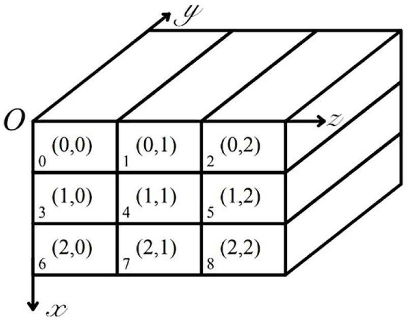
Figure 1: The division of the computational volume using a two-dimensional Cartesian topology (x-z plane).

Both the HIE-FDTD method and the FDTD method must solve the boundary condition problem. Therefore, it is important to determine the necessary components to transmit after the equal distribution of the problem.

For the FDTD method, updating field components at $(i,j,k)$ is dependent on the surrounding field components. To provide an example, as shown by Fig. 2, the iteration of $E_x$ component at $(i+1\mathrm{/}2,j,k)$ requires $H_z$ at $(i+1\mathrm{/}2,j+1\mathrm{/}2,k)$, $(i+1\mathrm{/}2,j-1\mathrm{/}2,k)$ and $H_y$ at $(i+1\mathrm{/}2,j-1\mathrm{/}2,k)$, $(i+1\mathrm{/}2,j+1\mathrm{/}2,k)$.

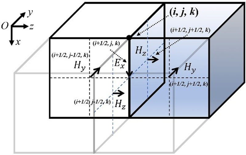
Figure 2: The iteration of $E_x$ component at $(i+1/2,j,k)$ using the conventional FDTD method and the surrounding field components.

Figure 3 shows that only the components encapsulated by the blue dotted contour designated to PROC4 are assigned in the parallel FDTD method. So, to update $E_x$ component in PROC4, $H_y$ component from PROC3 is required. As there is no division along the $y$-direction, there is no need to transmit $H_z$ component. Similarly, updating $E_z$ component requires $H_y$ component in PROC1, and updating $E_y$ component requires both $H_z$ and $H_x$ components in PROC1 and PROC3. It should be noted that PROC4 fulfils the role of both an emitter and an addressee process, and therefore, must send the components to the surrounding processes. The send-receive communications of PROC4 are illustrated in Fig. 3.

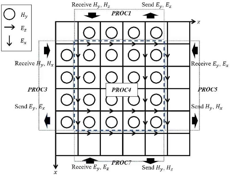
Figure 3: The send-receive communications in PROC4 using the parallel FDTD method.

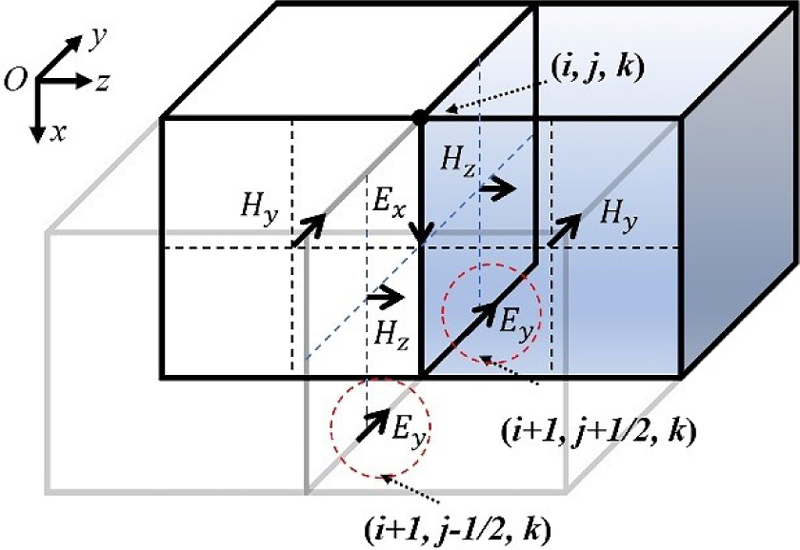
Figure 4: The iteration of $E_x$ component at $(i+1/2,j,k)$ using HIE-FDTD method and the surrounding field components.

Figure 4 shows the iteration of $E_x$ at $(i+1/2,j,k)$ using the HIE-FDTD method. $E_y$ at $(i+1,j+1/2,k)$ and $(i+1,j-1/2,k)$ are also essential, besides $H_y$ and $H_z$ components that are required in the FDTD method. Therefore, when implementing the parallel HIE-FDTD method, it is important to note that updating $E_x$ component requires $E_y$ belonging to PROC7, with $H_y$ component belonging to PROC3. To update $E_z$, it is necessary to receive $E_y$ component belonging to PROC5, with $H_y$component from PROC1.

Figure 5 (a) shows the complete communications between PROC4 and other processes in the parallel HIE-FDTD method. Figure 5 (b) shows that the parallel HIE-FDTD method requires the communication of $E_y$ component in the x- and z-directions when performing $E_x$ and $E_z$ iterations. It is the difference between it and the parallel FDTD method.

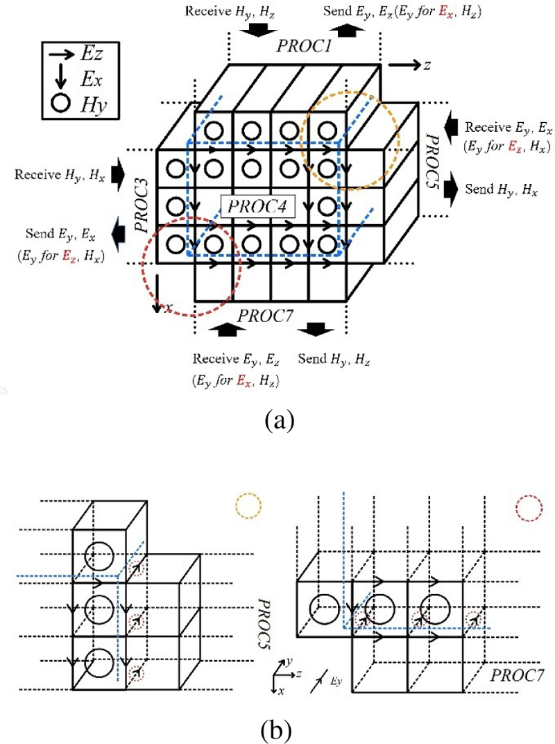
Figure 5: The communications between PROC4 and its neighboring processes using the parallel HIE-FDTD method: (a) Overall view and (b) the communication of $E_y$component in the x- and z-directions.

Assuming that the size of the field components array is $\mathrm{sizex}\times \mathrm{sizey}\times \mathrm{sizez}$, which needs to be augmented for the reception of the components from neighboring processes as follows,

$$A_i(\mathrm{sizex},\mathrm{sizey},\mathrm{sizez})\to A_i(\mathrm{sizex}+1,\mathrm{sizey},\mathrm{sizez}+1),$$

where $A=[E,H]$ and $i=[x,y,z]$.

The details of the derived data types implementation, transmission, and reception of field components are documented in [3]. The procedure for the parallel HIE-FDTD method is provided here:

1) MPI initialization

2) Read parameters used in simulation

3) Create a two-dimensional Cartesian topology (no division along the y-direction)

4) Create the derived data types for communications

5) Start updating field components

Update $E_y$ component

Communicate $E_y$ component for updating of $E_x$ and $E_z$components

Update $E_x$ and $E_z$ components

Communicate $E_x$ and $E_z$ components

Update the $H$-field components

Communicate the $H$-field components

6) End.

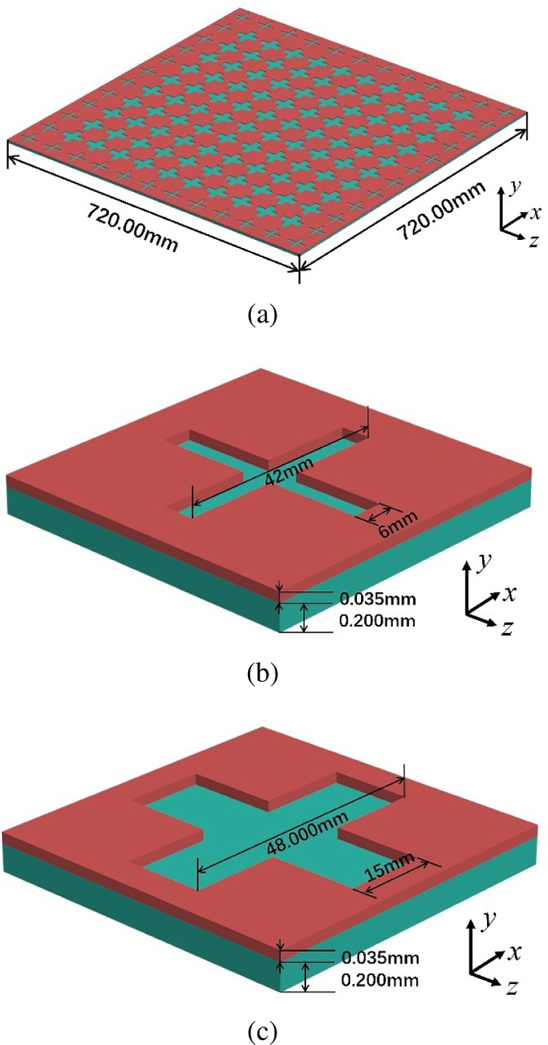
Figure 6: The structure of the FSS: (a) overall view of the FSS, (b) the size of the narrow cross slot unit, and (c) the size of the wide cross slot unit.

IV. NUMERICAL RESULTS

To verify the accuracy and efficiency of the implementation of the proposed parallel HIE-FDTD method based on the MPI library, a numerical example of a FSS is simulated. Figure 6 (a) shows the structure of the FSS. Its length in both x- and z-directions is 720 mm. The surface comprises two different cross-slot units, as shown in Figs. 6 (b) and (c).

The narrow cross slot has a width of 6 mm and a length of 42 mm, and the wide cross slot has a width of 15 mm and a length of 48 mm. The thickness of the FSS is 0.235 mm, of which metal is 0.035 mm thick and the substrate is 0.2 mm thick. The ${\epsilon }_r$ of the substrate is 4.5 and $\sigma$ is 0.004 S/m. The thickness of the metal is the fine structure of the FSS which greatly confines the computational efficiency. A plane wave polarized along the x-direction is incident perpendicular to the FSS. The excitation source is a modulated Gaussian pulse with a frequency range from 2.5 GHz to 4 GHz. The time dependence of the excitation function is given asfollows:

$$E_x\left(t\right)=\cos \left(2\pi \cdot fre\cdot t\right)\exp \left(-4\pi {\left(\left(t-t_0\right)\mathrm{/}\tau \right)}^2\right),$$

(13)

where $fre$ = 3.125 GHz, $\tau$ = 2.67 ns, and $t_0=0.9\tau =2.4$ ns.

One observation point is located at 120 mm behind the center of the surface. We use the serial FDTD, the serial HIE-FDTD method, and the parallel HIE-FDTD method to compute the electric field at the observation point and the transmission coefficient of the FSS. The minimum grids in the x- and z-directions are 1 mm. In the y-direction, the minimum grid is 0.035 mm. The total number of grids is 396$\times$35$\times$396. According to the time stability condition, the time step size in the FDTD method is

$\mathrm{\Delta }{t}_f=1\mathrm{/}c\sqrt{1\mathrm{/}\mathrm{\Delta }{x}^2+1\mathrm{/}\mathrm{\Delta }{y}^2+1\mathrm{/}\mathrm{\Delta }{z}^2}=$0.0583 ps, while in the HIE-FDTD method, the time step is

$\mathrm{\Delta }t=1\mathrm{/}c\sqrt{1\mathrm{/}\mathrm{\Delta }{x}^2+1\mathrm{/}\mathrm{\Delta }{z}^2}=$2.36 ps, which is 40.48 times larger than that in the FDTD method. The simulation history is 8 ns, which can ensure the complete convergence of time-domain signals. It corresponds to 323,842 time steps in the FDTD method and 8000 time steps in the HIE-FDTD method. The simulation is implemented on Intel(R) Xeon(R) Gold 6248R with 3.00 GHz CPU and 1 TB memory.

Figure 7 shows the value of $E_x$ component at the observation point calculated by using the parallel HIE-FDTD method, the serial HIE-FDTD method, and the serial FDTD method. Figure 8 presents the calculated transmission coefficient of the FSS. From these figures, it is obvious that the calculated results of the parallel HIE-FDTD agree very well with those of the serial HIE-FDTD method and the serial FDTD method, whether in the time domain or frequency domain. The transmission coefficient of the FFS exceeds 0.9 within the range from 2.9 GHz to 3.65 GHz. Figures 7 and 8 validate the high computational accuracy of the parallel HIE-FDTD method.

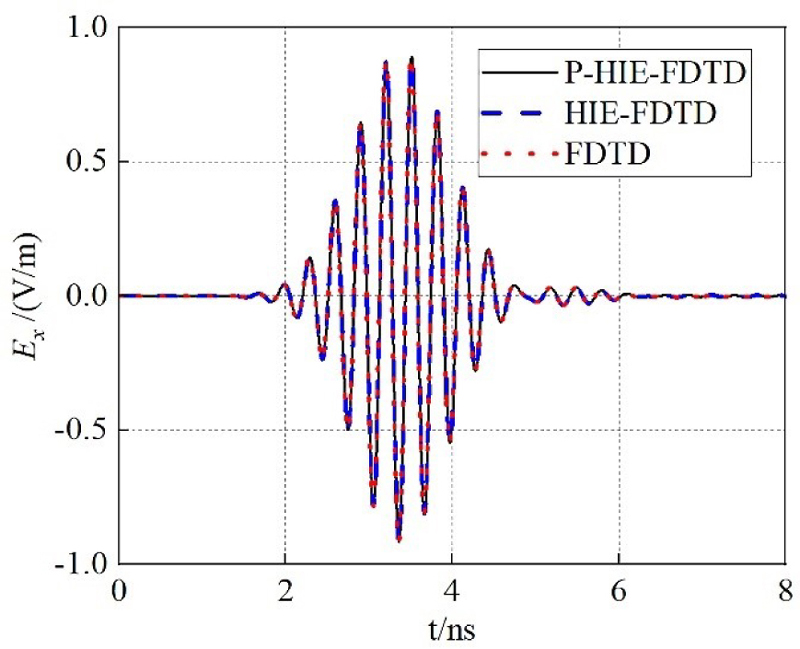
Figure 7: The value of the $E_x$ components at the observation point calculated by using the proposed parallel HIE-FDTD method, the serial HIE-FDTD method, and the serial FDTD method.

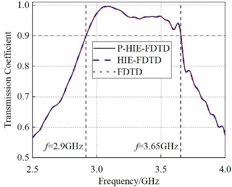
Figure 8: The result of the transmission coefficient of the FSS calculated by using the proposed parallel HIE method, the serial HIE-FDTD method, and the serial FDTD method.

Table 1 displays the computation time of the serial FDTD method, the serial HIE-FDTD method, and the parallel HIE-FDTD method with 32 processes. We also introduce the speedup factors $S_p\left(k\right)$ with the following definition:

$$S_p(k)=\frac{p\times \mathrm{Run}\mathrm{time}\mathrm{with}p\mathrm{cores}}{\mathrm{Run}\mathrm{time}\mathrm{with}k\mathrm{cores}},$$

(14)

where $p$ is the reference number of processors and $k$ is the number of processors used in calculation. $S_1\left(k\right)$of the proposed method is showed in Fig. 9.

The results demonstrate that the simulation speed of the serial HIE-FDTD method is 29.3 times faster than the serial FDTD, which is due to the larger time step in the HIE-FDTD method. Moreover, the simulation speed of the proposed parallel HIE-FDTD method with 32 processes is 25 times faster than the serial HIE-FDTD method. The parallel efficiency of the proposed method reaches 81.2 %. It can conclude that the proposed parallel HIE-FDTD method considerably reduces the runtime over the serial FDTD and the serial HIE-FDTD, while the accuracy of the proposed method is still maintained.

Table 1: The time step size, total time steps, and computing time of different methods

Method	$\mathbf{\Delta }\mathit{t}(\mathit{p}\mathit{s})$	Total Steps	Computing	Time (h)
FDTD	0.0583	323,842	901.40
HIE-FDTD	2.36	8000	30.77
P-HIE-FDTD	2.36	8000	1.18

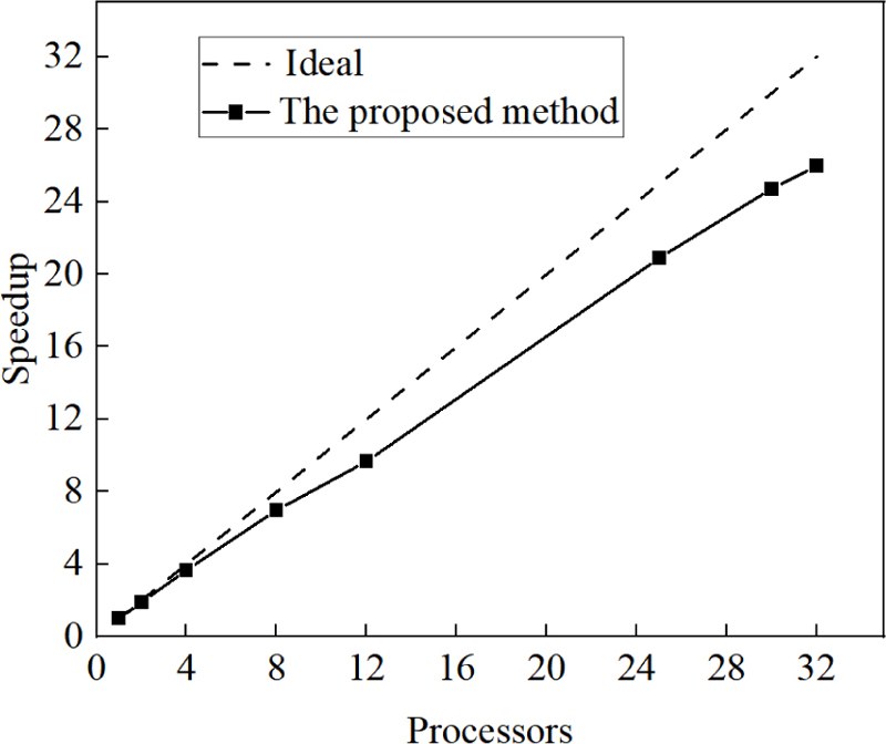
Figure 9: $S_1\left(k\right)$ obtained for a space size of 396$\times$35$\times$396 in case of the proposed parallel HIE-FDTD method.

Table 2: Comparison of computation efficiency

Number of Processes	Number of Subdomains	Computing Time (s)	Parallel Efficiency
1	$1\times 1\times 1$	6652.02	$100\%$
2	$2\times 1\times 1$	3496.58	$95.1\%$
4	$2\times 1\times 2$	1812.13	$91.8\%$
8	$4\times 1\times 2$	952.54	$87.3\%$
12	$4\times 1\times 3$	687.61	$80.6\%$
25	$5\times 1\times 5$	318.16	$83.6\%$
30	$6\times 1\times 5$	268.99	$82.4\%$
32	$8\times 1\times 4$	256.00	$81.2\%$

The parallel efficiency of the proposed method is defined as $\delta =T_1\mathrm{/}{T}_{n}n$. Here, $T_1$ represents the computing time of the HIE-FDTD method with a single process; n is the number of the processes and $T_n$ is the computing time of the HIE-FDTD method with n processes. Table 2 presents the computing time and the parallel efficiency of the proposed parallel HIE-FDTD method. It can be observed that the efficiency maintains above 80% for different numbers of processes, which proves that this method is very suitable for parallel computing.

V. CONCLUSION

This paper describes a parallel HIE-FDTD method implemented through the MPI library. Parallel computing is realized by creating a two-dimensional topology that divides the computational volume along two directions. The differences of the field components transmitted between the parallel HIE-FDTD method and parallel FDTD method are discussed. The function for communication and derived data types provided by the MPI library are employed to transmit HIE-FDTD field components. The numerical example indicates the high computational accuracy and excellent parallel efficiency of the proposed method. It shows that the parallel efficiency maintains above 80% for different numbers of processes, which proves that this method is very suitable for parallel computing.

ACKNOWLEDGMENT

This work was supported by the National Key Research and Development Program of China under No. 2020YFA0709800, and by the National Natural Science Foundations of China under No. 62122061, and also by the Shaanxi Natural Science Basic Research Project under No. 2023-JC-QN-0673.

REFERENCES

[1] K. S. Yee, “Numerical solution of initial boundary value problems involving Maxwell’s equations in isotropic media,” IEEE Trans. Antennas Propagat., vol. AP-14, pp. 302-307, 1966.

[2] A. Taflove and S. C. Hagness, Computational Electrodynamics: The Finite-Difference Time-Domain Method, 3rd ed. Boston, MA, USA: Artech House, 2005.

[3] Guiffaut and K. Mahdjoubi, “A parallel FDTD algorithm using the MPI library,” IEEE Antennas Propag. Mag., vol. 43, no. 2, pp. 94-103, Apr. 2001.

[4] T. Namiki, “A new FDTD algorithm based on alternating-direction implicit method,” IEEE Trans. Microw. Theory Tech., vol. 47, no. 10, pp. 2003-2007, Oct. 1999.

[5] Y. Yang, R. S. Chen, and E. K. N. Yung, “The unconditionally stable Crank–Nicolson FDTD method for three-dimensional Maxwell’s equations,” Microw. Opt. Tech. Lett., vol. 39, pp. 97-101, Oct. 2003.

[6] J. Shibayama, M. Muraki, J. Yamauchi, and H. Nakano, “Efficient implicit FDTD algorithm based on locally one-dimensional scheme,” Electron. Lett., vol. 41, no. 19, pp. 1046-1047, Sep. 2005.

[7] S. Garcia, T. Lee, and S. Hagness, “On the accuracy of the ADI-FDTD method,” IEEE Antennas Wireless Propag. Lett., vol. 1, no. 1, pp. 31-34, Jan. 2002.

[8] M. Li, K. P. Ma, D. M. Hockanson, J. L. Drewniak, T. H. Hubing, and T. P. Van Doren, “Numerical and experimental corroboration of an FDTD thin slot model for slots near corners of shielding enclosures,” IEEE Trans. Electromagn. Compat., vol. 39, no. 3, pp. 225-232, Aug. 1997.

[9] J. Chen and J. G. Wang, “A 3D hybrid implicit-explicit FDTD scheme with weakly conditional stability,” Microw. Opt. Technol. Lett. 48, 2291-2294, 2006.

[10] J. Chen and J. Wang, “Comparison between HIE-FDTD method and ADI FDTD method,” Microw. Opti. Technol. Lett., vol. 49, no. 5, pp. 1001-1005, Mar. 2007.

BIOGRAPHIES

Qin Nan was born in Yan’an, China. He completed his B.S. in Northwest University, Xi’an, China, in 2022. He is currently working toward the Ph.D. degree in electromagnetic field and microwave technology at Xi’an Jiaotong University, Xi’an, China. His research interests include the fast FDTD method and parallel computing.

Chunhui Mou was born in Yantai, China. She received the B.S. and M.S. degrees from Xidian University, Xi’an, China, in 2012 and 2015, and the Ph.D. degree from Xi’an Jiaotong University, Xi’an, China, in 2023, all in electromagnetic field and microwave technology.

She is currently working in Xi’an Jiaotong University, Xi’an, China, as a postdoctoral researcher. Her research interests include the fast FDTD method, FDTD mesh generation method, and multi-physical field calculation.

Juan Chen was born in Chongqing, China. She received the Ph.D. degree from Xi’an Jiaotong University, Xi’an, China, in 2008, in electromagnetic field and microwave technology.

She is currently working in Xi’an Jiaotong University, Xi’an, China, as a professor. Her research interests include computational electromagnetics, microwave device design, etc.

ACES JOURNAL, Vol. 38, No. 11, 849–856
doi: 10.13052/2023.ACES.J.381103
© 2023 River Publishers

ABSTRACT

I. INTRODUCTION

II. THEORY OF THE HIE-FDTD METHOD

III. PARALLELISM WITH THE MPI LIBRARY

IV. NUMERICAL RESULTS

V. CONCLUSION

ACKNOWLEDGMENT

REFERENCES

BIOGRAPHIES