Near Field Scatter from a Body of Revolution

Edward C. Michaelchuck Jr.${}^{\mathbf{\text{1}}}$, Samuel G. Lambrakos${}^{\mathbf{\text{2}}}$, and William O. Coburn${}^{\mathbf{\text{3}}}$

¹Signature Technology Office

²Space Systems Development Division
U.S. Naval Research Laboratory, Washington, D.C. 20375, USA
edward.c.michaelchuck.civ@us.navy.mil, samuel.g.lambrakos.civ@us.navy.mil

³Retired Electronics Engineer
Army Research Laboratory, Adelphi, MD 20378, USA
keefecoburn@comcast.net

Submitted On: January 19, 2024; Accepted On: June 21, 2024

ABSTRACT

Better understanding of electromagnetic wave propagation through vegetation and forest environments can be achieved with the aid of modeling and simulation. Specifically, modeling the coherent summation of electromagnetic waves due to both single scatter and multi-scatter effects. To accurately perform simulations in lower frequency bands, S-band and below, the Body of Revolution (BOR) Method of Moments (MoM) must be extended to calculate the scattered electric and magnetic near-fields from BOR in the presence of a plane wave. The near field interactions specifically occur during the various higher order scattering harmonics, i.e. 2${}^{\mathrm{nd}}$ order and greater harmonics. Additionally, the method must accurately capture scattered fields in the presence of a non-plane wave incident upon BOR. The focus of this study is modeling lossy dielectric BOR that are characteristic of vegetation and forest environments, e.g., cylinders representing tree branches. Although the formal electric and magnetic field scattering definitions are known, this report presents analytical formulations of near field scattering from BOR for this implementation of BOR-MoM. The scattered-field extensions are validated using the commercial software FEKO©, which simulates electromagnetic-wave scattering in 3D using MoM formulation of scattered fields.

Index Terms: Body of Revolution, Method of Moments, near fields, remote sensing, scattering.

I. INTRODUCTION

Accurate modeling and simulation of electromagnetic wave scattering from vegetation within forest environments is essential for various remote sensing and communications applications including Synthetic Aperture RADAR imaging and cellular connectivity. These models should consider the coherent single and multi-path effects of electromagnetic waves propagating through environments consisting of vegetation and forests. These effects can be described using Multiple Scattering Theory (MST) [1]. Previously, multi-scatter has been characterized through shooting bounce ray methodologies where the physical optics approximations apply, $\lambda \ll d$, where d is the maximum size of the scattering object [1–3]. These methodologies, however, are not suitable when the physical optics approximation no longer applies, i.e., objects in the scene are not sufficiently electrically large.

Other methods that have been studied include iterative radiative transfer methods and Fresnel double scattering using Discrete Dipole Approximation [4, 5]. Full wave solutions have also been used to examine multiple scattering effects in trees. The software FEKO©, which is for simulation of electromagnetic-wave scattering in 3D using the Method of Moments (MoM) formulation of scattered fields, was used to examine scattering from electrically small vegetation above a dielectric ground plane [6]. Additionally, a two-step hybrid method was employed, combining (1) 3D MoM (via FEKO©) to fill in the T-Matrix coefficients for the individual scatterers and (2) MST [7]. These modeling efforts [6, 7] showed exceptional results, but were not suited for the study of large stochastic forest environments due to computational requirements. Accordingly, these efforts have motivated the need for faster simulation of wave propagation through vegetation and forest environments, using MoM formulation of Maxwell’s Equations.

Traditionally, trees and vegetation are characterized by axi-symmetric objects, e.g., cylinders, which allows for the use of the Body of Revolution (BOR) MoM [1–8]. The classical BOR-MoM provides a full wave solution to scattering phenomenon for incident plane waves [9–23]. Since the method only discretizes over an analytically singular generating arc for a set of harmonics, the computational burden is an order of magnitude less than that of the traditional 3D MoM. In turn, BOR-MoM provides a fast, accurate solution for BOR. Additionally, it allows for the calculation of both near fields and far fields from the induced electric and fictitious magnetic surface currents. Previous applications of BOR-MoM analyzed singular scatterers with respect to an incident field [9–22]. These analyses included: far field electric and magnetic field expansions [9–23], RADAR Cross Section (RCS) analysis using the scattering amplitude [13, 17, 20], expansion of the integral formulation to consider a dielectric medium surrounding BOR in a layered system [15], and evaluation of the resonances of a BOR in a lossy dispersive half-space [11–12, 15]. Typically, these methodologies considered only a single scatterer or integral expansions to BOR derivation to handle multi-reflection/scatter effects that can occur in a scene.

Due to the stochastic nature of trees and foliage however, expansion of the integral operators to account for the connections between the branches is not well posed computationally, in terms of discrete numerical representation. Additionally, BOR-MoM is primarily used for single objects, and not multiple discrete scatterers, within a scene. Thus, various scatterers must interact via multi-scatter techniques rather than via integral operator additions in the impedance matrix. In turn, the nature of foliage is that of Multiple BOR (MBOR) scattering which has been extensively researched and applied to foliage [24–31]. These techniques include various methods such as cylindrical and spherical wave expansions, T-matrix approximations, and thin cylinder approximations [25–31]. To flush out the subtleties of tree scattering using MBOR approaches, however, these methods are not ideal for physically and accurately understanding the mechanisms by which the waves propagate through foliage mediums and interact when minimal assumptions are present.

To analyze these multi-scatter effects, both near field and far field scattered electromagnetic waves must be analyzed for both plane wave and non-plane wave incidence. The non-plane wave case occurs when a branch scatters onto another branch that is within the near field; the resultant incident wave upon the second branch has a specific wave front, assumed non-plane wave, across the branch [5–7].

In what follows, the focus of this paper is near field scattering from a BOR. Although the formal electric and magnetic field scattering definitions are known, this paper provides a detailed derivation of the formal scattering for this particular implementation of BOR-MoM. Note that the near field derivation is valid for all of space; however, it is not computationally advantageous to use it when in the far field for a scatterer. First, presented is a derivation for BOR-MoM. Secondly, the generalized scattered fields for all of space - including the near fields - are derived for this implementation of BOR-MoM. Then the near field calculation method is validated for both perfect electric conductors (PEC) and lossy dielectric cylinders against the 3D MoM in FEKO©.

II. BODY OF REVOLUTION METHOD OF MOMENTS

BOR is the rotation of a generating curve, planar arc C, about an axis, see Fig. 1. In this study, the axis of rotation will be the z-axis of a Cartesian coordinate system, and the generating curve will only exist in the right half plane where by definition the curve is rotated 360${}^o$ around the z-axis. In turn, the surface, S, formed by BOR will be the interface separating free space and the scatterer with material properties $ϵ={ϵ}_{\mathrm{r}}{ϵ}_0$ and $\mu ={\mu }_{\mathrm{r}}{\mu }_0$.

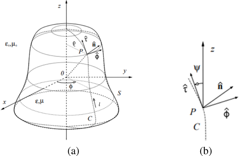
Figure 1: A Body of Revolution where (a) is the three-dimensional model with the relevant coordinate system definitions and (b) is the coordinate definitions along the surface of BOR. Note that the BOR figure representation is from and with permission of Matthaeis and Lang [10, 11].

The coordinate unit vectors are defined in Fig. 1 by:

	$\widehat{\mathit{\tau }}$	$=\sin \psi \cos \phi \widehat{\mathbf{x}}+\sin \psi \sin \phi \widehat{\mathbf{y}}+\cos \psi \widehat{\mathbf{z}},$		(1)
	$\widehat{\mathbf{n}}$	$=\cos \psi \cos \phi \widehat{\mathbf{x}}+\cos \psi \sin \phi \widehat{\mathbf{y}}-\sin \psi \widehat{\mathbf{z}},$		(2)
	$\widehat{\mathit{\phi }}$	$=-\sin \phi \widehat{\mathbf{x}}+\cos \phi \widehat{\mathbf{y}}.$		(3)

The Electric Field Integral Equations (EFIE) used to evaluate the surface currents along the surface, S, are defined by:

	${\displaystyle \frac{{\mathbf{E}}_{\mathrm{t}}(\mathbf{r})}{2}}={\mathbf{E}}_{\mathrm{t}}^{\mathrm{i}}(\mathbf{r})+$
	$\mathrm{\hspace{1em}}-\mathrm{j}\omega {\mu }_0(\underset{¯}{\mathbf{I}}-\widehat{\mathbf{n}}\widehat{\mathbf{n}})\cdot \mathrm{PV}{\displaystyle \underset{{\mathrm{s}}^{+}}{\int }}\underset{¯}{\mathbf{G}}(\mathbf{r},{\mathbf{r}}^{\prime })\cdot {\mathbf{J}}_{\mathrm{s}}\left({\mathbf{r}}^{\prime }\right)d{S}^{\prime }+$
	$\mathrm{\hspace{1em}}-(\underset{¯}{\mathbf{I}}-\widehat{\mathbf{n}}\widehat{\mathbf{n}})\cdot \mathrm{PV}{\displaystyle \underset{{\mathrm{s}}^{+}}{\int }}\underset{¯}{\mathbf{K}}(\mathbf{r},{\mathbf{r}}^{\prime })\times {\mathbf{M}}_{\mathrm{s}}\left({\mathbf{r}}^{\prime }\right)\mathrm{dS}{S}^{\prime },$		(4)

	${\displaystyle \frac{{\mathbf{E}}_{\mathrm{t}}(\mathbf{r})}{2}}=\mathrm{j}\omega \mu (\underset{¯}{\mathbf{I}}-\widehat{\mathbf{n}}\widehat{\mathbf{n}})\cdot \mathrm{PV}{\displaystyle \underset{{\mathrm{s}}^{-}}{\int }}\underset{¯}{\mathbf{G}}(\mathbf{r},{\mathbf{r}}^{\prime })\cdot {\mathbf{J}}_{\mathbf{s}}\left({\mathbf{r}}^{\prime }\right){\mathrm{dS}}^{\prime }+$
	$\mathrm{\hspace{1em}}-(\underset{¯}{\mathbf{I}}-\widehat{\mathbf{n}}\widehat{\mathbf{n}})\cdot \mathrm{PV}{\displaystyle \underset{{\mathrm{S}}^{-}}{\int }}\underset{¯}{\mathbf{K}}(\mathbf{r},{\mathbf{r}}^{\prime })\times {\mathbf{M}}_{\mathrm{s}}\left({\mathbf{r}}^{\prime }\right)\mathrm{dS}{S}^{\prime },$		(5)

where ${\mathbf{E}}_{\mathrm{t}}(\mathbf{r})$ is the tangential field on the surface, $\omega$ is the angular frequency, $\underset{¯}{\mathbf{I}}$ is the unit dyadic, PV denotes a principal value integral, ${\mathrm{S}}^{+}$is the outer surface of $\mathrm{S},{\mathrm{S}}^{-}$ is the inner surface of $S,\underset{¯}{\mathbf{G}}(\mathbf{r},{\mathbf{r}}^{\prime })$ is the electric dyadic Green’s function, $\underset{¯}{\mathbf{K}}(\mathbf{r},{\mathbf{r}}^{\prime })$ is the magnetic dyadic Green’s function, ${\mathbf{J}}_{\mathrm{s}}\left({\mathbf{r}}^{\prime }\right)$ are the induced electric surface currents, and ${\mathbf{M}}_{\mathrm{s}}\left({\mathbf{r}}^{\prime }\right)$ are the induced, fictitious magnetic surface currents.

The incident fields and induced sources within EFIE can then be split into $\tau$ and $\mathit{\phi }$ vector components:

	${\mathbf{E}}_{\mathrm{t}}^{\mathrm{i}}(\mathbf{r})$	$={\mathrm{E}}_{\tau }^{\mathrm{i}}(\mathrm{l},\phi )\widehat{\mathit{\tau }}+{\mathrm{E}}_{\phi }^{\mathrm{i}}(\mathrm{l},\phi )\widehat{\mathit{\phi }},$		(6)
	${\mathbf{J}}_{\mathrm{s}}(\mathbf{r})$	$={\mathrm{J}}_{\tau }(\mathrm{l},\phi )\widehat{\mathit{\tau }}+{\mathrm{J}}_{\phi }(\mathrm{l},\phi )\widehat{\mathit{\phi }},$		(7)
	${\mathbf{M}}_{\mathrm{s}}(\mathbf{r})$	$={\mathrm{M}}_{\tau }(\mathrm{l},\phi )\widehat{\mathit{\tau }}+{\mathrm{M}}_{\phi }(\mathrm{l},\phi )\widehat{\mathit{\phi }},$		(8)

where $\mathrm{l}$ denotes the location on generating arc, C.

A. Fourier series expansion

To evaluate the induced surface currents on the generating arc, EFIE are expanded in Fourier series around the z-axis such that MoM is only evaluated over the generating arc for a series of harmonics. The resulting induced sources are:

	$\mathrm{E}_{\mathrm{p}}{}^{\mathrm{i}}(\mathbf{r})$	$={\displaystyle \sum _{\mathrm{n}=-\mathrm{\infty }}^{\mathrm{\infty }}}\mathrm{E}_{\mathrm{p},\mathrm{n}}{}^{\mathrm{i}}{\mathrm{e}}^{\mathrm{jn}\phi },$		(9)
	${\mathrm{J}}_{\mathrm{p}}(\mathbf{r})$	$={\displaystyle \sum _{\mathrm{n}=-\mathrm{\infty }}^{\mathrm{\infty }}}{\mathrm{J}}_{\mathrm{p},\mathrm{n}}{\mathrm{e}}^{\mathrm{jn}\phi },$		(10)
	${\mathrm{M}}_{\mathrm{p}}(\mathbf{r})$	$={\displaystyle \sum _{\mathrm{n}=-\mathrm{\infty }}^{\mathrm{\infty }}}{\mathrm{M}}_{\mathrm{p},\mathrm{n}}{\mathrm{e}}^{\mathrm{jn}\phi },$		(11)

where $\mathrm{p},\mathrm{q}=\tau ,\phi$ and the Fourier Series Coefficients are defined as:

$${\mathrm{C}}_{\mathrm{n}}=\frac{1}{2\pi }\underset{-\pi }{\overset{\pi }{\int }}\mathrm{f}(\phi ){\mathrm{e}}^{-\mathrm{jn}{\phi }^{\prime }}d{\phi }^{\prime },$$

(12)

for $\mathrm{f}\left(\phi \right)=\mathrm{E},\mathrm{J},\mathrm{M}$, etc.

B. Method of Moments expansion

Now the electric and magnetic surface currents can be discretized for MoM such that:

	${\mathrm{J}}_{\tau ,\mathrm{n}}\left(\mathrm{l}\right)$	$={\displaystyle \sum _{\mathrm{m}=1}^{\mathrm{N}}}{\mathrm{J}}_{\tau ,\mathrm{m},\mathrm{n}}={\displaystyle \sum _{\mathrm{m}=1}^{\mathrm{N}}}{\displaystyle \frac{{\mathrm{\Lambda }}_{\mathrm{m}}^{\tau ,\mathrm{n}}{\mathrm{P}}_{\mathrm{m}}\left(\mathrm{l}\right)}{{\rho }_{\mathrm{m}}}},$		(13)
	${\mathrm{J}}_{\phi ,\mathrm{n}}(\mathrm{l})$	$={\displaystyle \sum _{\mathrm{m}=1}^{\mathrm{N}}}{\mathrm{J}}_{\phi ,\mathrm{m},\mathrm{n}}={\displaystyle \sum _{\mathrm{m}=1}^{\mathrm{N}+1}}{\mathrm{\Lambda }}_{\mathrm{m}}^{\phi ,\mathrm{n}}{\mathrm{P}}_{\mathrm{m}}\left(\mathrm{l}\right),$		(14)
	${\mathrm{M}}_{\tau ,\mathrm{n}}\left(\mathrm{l}\right)$	$={\displaystyle \sum _{\mathrm{m}=1}^{\mathrm{N}}}{\mathrm{M}}_{\tau ,\mathrm{m},\mathrm{n}}={\displaystyle \sum _{\mathrm{m}=1}^{\mathrm{N}}}{\mathrm{\Omega }}_{\mathrm{m}}^{\tau ,\mathrm{n}}{\mathrm{P}}_{\mathrm{m}}\left(\mathrm{l}\right),$		(15)
	${\mathrm{M}}_{\phi ,\mathrm{n}}\left(\mathrm{l}\right)$	$={\displaystyle \sum _{\mathrm{m}=1}^{\mathrm{N}}}{\mathrm{M}}_{\tau ,\mathrm{m},\mathrm{n}}={\displaystyle \sum _{\mathrm{m}=1}^{\mathrm{N}+1}}{\mathrm{\Omega }}_{\mathrm{m}}^{\phi ,\mathrm{n}}{\mathrm{P}}_{\mathrm{m}}\left(\mathrm{l}\right),$		(16)

where ${\mathrm{J}}_{\tau ,\mathrm{m},\mathrm{n}},{\mathrm{J}}_{\phi ,\mathrm{m},\mathrm{n}},{\mathrm{M}}_{\tau ,\mathrm{m},\mathrm{n}}$, and ${\mathrm{M}}_{\tau ,\mathrm{m},\mathrm{n}}$ are the surface currents per harmonic for their respective polarization vector on each discretized segment of the generating arc, $m$ is the segment number, $N$ is the total number of segments, ${\mathrm{P}}_{\mathrm{m}}(1)$ is the chosen basis function expansion, ${\rho }_{\mathrm{m}}$ is the distance from the $z$-axis, and ${\mathrm{\Lambda }}_{\mathrm{m}}^{\tau ,\mathrm{n}},{\mathrm{\Lambda }}_{\mathrm{m}}^{\phi ,\mathrm{n}},{\mathrm{\Omega }}_{\mathrm{m}}^{\tau ,\mathrm{n}}$, and ${\mathrm{\Omega }}_{\mathrm{m}}^{\phi ,\mathrm{n}}$ are the basis function coefficients.

Testing functions are now applied using the symmetric product:

$$\begin{array}{c}\hfill ⟨\chi \left(\mathrm{l}\right),\alpha \left(\mathrm{l}\right)⟩={\int }_{-\mathrm{\infty }}^{\mathrm{\infty }}\chi \left(\mathrm{l}\right)\cdot \alpha \left(\mathrm{l}\right)\mathrm{dl}.\hfill \end{array}$$

(17)

Now the interaction matrix and incident field matrix can be evaluated for a signal harmonic on BOR generating arc. The equivalent sources are solved by inverting the interaction matrix:

$$\begin{array}{c}\hfill \left[{\mathrm{J}}_{\mathrm{n}}\right]={\left[{\mathrm{Z}}_{\mathrm{n}}\right]}^{-1}\left[{\mathrm{E}}_{\mathrm{n}}\right].\hfill \end{array}$$

(18)

III. SCATTERED FIELD EQUATIONS FOR A BODY OF REVOLUTION

The scattered field definition using equivalent sources is:

	${\mathbf{E}}^{\mathrm{s}}(\mathbf{r})$	$=-\mathrm{j}\omega {\mu }_0{\displaystyle \oint {\underset{¯}{\mathbf{G}}}^0(\mathbf{r},{\mathbf{r}}^{\prime })\cdot {\mathbf{J}}_{\mathrm{s}}\left(r^{\prime }\right){\mathrm{dS}}^{\prime }}+$
		$\mathrm{\hspace{1em}}-{\displaystyle \oint {\underset{¯}{\mathbf{K}}}^0(\mathbf{r},{\mathbf{r}}^{\prime })\cdot {\mathbf{M}}_{\mathrm{s}}\left({\mathbf{r}}^{\prime }\right){\mathrm{dS}}^{\prime }},$		(19)
	${\mathbf{H}}^{\mathrm{s}}(\mathbf{r})$	$={\displaystyle \oint {\underset{¯}{\mathbf{K}}}^0(\mathbf{r},{\mathbf{r}}^{\prime })\cdot {\mathrm{J}}_{\mathrm{s}}\left({\mathbf{r}}^{\prime }\right){\mathrm{dS}}^{\prime }}+$
		$\mathrm{\hspace{1em}}-j\omega {ϵ}_0{\displaystyle \oint {\underset{¯}{\mathbf{G}}}^0(\mathbf{r},{\mathbf{r}}^{\prime })\cdot {\mathbf{M}}_{\mathrm{s}}\left({\mathbf{r}}^{\prime }\right){\mathrm{dS}}^{\prime }},$		(20)

where ${\mathbf{E}}^{\mathrm{s}}(\mathbf{r})$ is the scattered electric field, ${\mathbf{H}}^{\mathrm{s}}(\mathbf{r})$ is the scattered magnetic field, $r$ is the scattered field location, and ${\mathbf{r}}^{\prime }$ is the surface current source location. Note that equations (19) and (20) are derived from the general formulation, ${\mathbf{E}}^{\mathrm{s}}(\mathbf{r})={\mathbf{E}}^{\text{total}}(\mathbf{r})-{\mathbf{E}}^{\text{inc}}(\mathbf{r})$. The dyadic Green’s functions are defined as:

	${\underset{¯}{\mathbf{G}}}^0(\mathbf{r},{\mathbf{r}}^{\prime })$	$=\left(\underset{¯}{\mathbf{I}}+{\displaystyle \frac{\nabla \nabla }{{\mathrm{k}}^2}}\right){\mathrm{g}}^0(\mathbf{r},{\mathbf{r}}^{\prime }),$		(21)
	${\underset{¯}{\mathbf{K}}}^0(\mathbf{r},{\mathbf{r}}^{\prime })$	$=\nabla {\mathrm{g}}^0(\mathbf{r},{\mathbf{r}}^{\prime })\times \underset{¯}{\mathbf{I}},$		(22)

where:

$${\mathrm{g}}^0(\mathbf{r},{\mathbf{r}}^{{}^{\prime }})=\frac{{\mathrm{e}}^{-{\mathrm{jk}}_0\left|\mathbf{r}-{\mathbf{r}}^{{}^{\prime }}\right|}}{4\pi \left|\mathbf{r}-{\mathbf{r}}^{{}^{\prime }}\right|}.$$

(23)

Next, the scattered electric field equations, equation (19), are separated, i.e.:

	${\mathbf{E}}^{\mathrm{s}}(\mathbf{r})$	$=-j\omega {\mu }_0{\mathbf{E}}_1^{\mathrm{s}}(\mathbf{r})-{\mathbf{E}}_2^{\mathrm{s}}(\mathbf{r}),$		(24)
	${\mathbf{E}}_1^{\mathrm{s}}(\mathbf{r})$	$={\displaystyle \oint {\underset{¯}{\mathbf{G}}}^0(\mathbf{r},{\mathbf{r}}^{\prime })\cdot {\mathbf{J}}_s\left({\mathbf{r}}^{\prime }\right){\mathrm{dS}}^{\prime }},$		(25)
	${\mathbf{E}}_2^{\mathrm{s}}(\mathbf{r})$	$={\displaystyle \oint {\underset{¯}{\mathbf{K}}}^0(\mathbf{r},{\mathbf{r}}^{\prime })\cdot {\mathbf{M}}_{\mathrm{s}}\left({\mathbf{r}}^{\prime }\right){\mathrm{dS}}^{\prime }}.$		(26)

A. ${\mathbf{E}}_{\mathbf{1}}^{\mathbf{s}}\left(\mathbf{r}\right)$ integral expansion

The electric field integral operator for the electric surface currents, equation (25), can be combined with equations (7), (10), and (21) to yield:

$${\mathbf{E}}_1^s(\mathbf{r})=\sum _{\mathrm{n}=-\mathrm{\infty }}^{\mathrm{\infty }}{\mathbf{E}}_{1,\mathrm{n}}^{\mathrm{s}}\left\{{\mathbf{J}}_{\mathrm{s},\mathrm{n}}\left({\mathbf{l}}^{\prime }\right)\right\}{\mathrm{e}}^{\mathrm{j}{\phi }_s},$$

(27)

where ${\phi }_s$ is the azimuthal scattering angle. The Fourier series coefficients are:

$${\mathbf{E}}_{1,n}^S=\underset{S}{\int }{\underset{¯}{\mathbf{G}}}^0(\mathbf{r},\mathbf{r})\cdot \left({\mathbf{J}}_{\tau ,n}{\widehat{\mathit{\tau }}}^{\prime }+{\mathbf{J}}_{\phi ,n}{\widehat{\mathit{\phi }}}^{\prime }\right)e^{jn{\phi }^{\prime }}\mathit{d}{S}^{\prime }.$$

(28)

Next, performing the dot products of the dyadic Green’s function in spherical coordinates with the local BOR coordinate system, and separating the scattered field components into separate spherical components, $\widehat{\mathit{r}}$, $\widehat{\mathit{\phi }}$, and $\widehat{\mathit{\theta }}$, yields:

	${\mathbf{E}}_{1,n,r}^s$	$={\displaystyle \underset{S}{\int }}{g}^0(\mathbf{r},{\mathbf{r}}^{\prime })F_r\left({\mathbf{J}}_{s,n}\right)e^{jn{\phi }^{\prime }}\mathit{d}{S}^{\prime }\widehat{\mathbf{r}},$		(29)
	${\mathbf{E}}_{1,n,\phi }^s$	$={\displaystyle \underset{S}{\int }}{g}^0(\mathbf{r},{\mathbf{r}}^{\prime })F_{\phi }\left({\mathbf{J}}_{s,n}\right)e^{jn{\phi }^{\prime }}\mathit{d}{S}^{\prime }\widehat{\mathit{\phi }},$		(30)
	${\mathbf{E}}_{1,n,\theta }^s$	$={\displaystyle \underset{S}{\int }}{g}^0(\mathbf{r},{\mathbf{r}}^{\prime })F_{\theta }\left({\mathbf{J}}_{s,n}\right)e^{jn{\phi }^{\prime }}\mathit{d}{S}^{\prime }\widehat{\mathit{\theta }}.$		(31)

The definitions of $F_r$, $F_{\phi }$, and $F_{\theta }$ are given in Appendix I. Given derivation of the proper terms accounting for the angular dependencies of the two coordinate systems, equations (29-31) can be expanded further using MoM definitions, equations (13) and (14):

	${\mathbf{E}}_{1,n,r}^S$	$={\displaystyle \sum _{m=1}^N}{\displaystyle \underset{S}{\int }}{g}^0(\mathbf{r},{\mathbf{r}}^{\prime })F_r\left(J_{n,m}\right)e^{jn{\phi }^{\prime }}{e}^{-jn\phi }\mathit{d}{S}^{\prime }\widehat{\mathbf{r}},$		(32)
	${\mathbf{E}}_{1,n,\phi }^s$	$={\displaystyle \sum _{m=1}^N}{\displaystyle \underset{S}{\int }}{g}^0(\mathbf{r},{\mathbf{r}}^{\prime })F_{\phi }\left(J_{n,m}\right)e^{jn{\phi }^{\prime }}{e}^{-jn\phi }\mathit{d}{S}^{\prime }\widehat{\mathit{\phi }},$		(33)
	${\mathbf{E}}_{1,n,\theta }^s$	$={\displaystyle \sum _{m=1}^N}{\displaystyle \underset{S}{\int }}{g}^0(\mathbf{r},{\mathbf{r}}^{\prime })F_{\theta }\left(J_{n,m}\right)e^{jn{\phi }^{\prime }}{e}^{-jn\phi }\mathit{d}{S}^{\prime }\widehat{\mathit{\theta }}.$		(34)

Recognizing that the basis-function sets chosen are rectangular and triangular, and that the discretization is appropriately fine, the integration over a segment can be approximated by:

$$\underset{t_A}{\overset{t_B}{\int }}f\left(l^{\prime }\right)\mathit{d}{l}^{\prime }=\left(t_B-t_A\right)f\left(\frac{t_B-t_A}{2}\right).$$

(35)

Application of this approximation, with triangular basis functions, minimizes error if either side of the basis functions (left and right of the triangle) are evaluated independently. Using equation (35) and equations (32-34), the integration along the generating arc, $l$, over a single segment becomes:

	${\mathbf{E}}_{1,n,r,m}^s$	$=\mathrm{\Delta }{l}_{m,k}{\rho }_m{\displaystyle \underset{0}{\overset{2\pi }{\int }}}{g}^0(\mathbf{r},{\mathbf{r}}_m)F_{r,n,m}\left(J_{n,m}\right)e^{jn{\phi }^{\prime }}\mathit{d}{\phi }^{\prime }\widehat{\mathbf{r}},$		(36)
	${\mathbf{E}}_{1,n,\phi ,m}^s$	$=\mathrm{\Delta }{l}_{m,k}{\rho }_m{\displaystyle \underset{0}{\overset{2\pi }{\int }}}{g}^0(\mathbf{r},{\mathbf{r}}_m)F_{\phi ,n,m}\left(J_{n,m}\right)e^{jn{\phi }^{\prime }}\mathit{d}{\phi }^{\prime }\widehat{\mathit{\phi }},$		(37)
	${\mathbf{E}}_{1,n,\theta ,m}^s$	$=\mathrm{\Delta }{l}_{m,k}{\rho }_m{\displaystyle \underset{0}{\overset{2\pi }{\int }}}{g}^0(\mathbf{r},{\mathbf{r}}_{\mathbf{m}})F_{\theta ,n,m}\left(J_{n,m}\right)e^{jn{\phi }^{\prime }}\mathit{d}{\phi }^{\prime }\widehat{\mathit{\theta }}.$		(38)

Consistently, this reformulation has reduced the multivariable integration to that of a single integration around the $\phi$-axis.

B. ${\mathbf{E}}_{\mathbf{2}}^{\mathbf{s}}\left(\mathbf{r}\right)$ integral expansion

As for equation (27), ${\mathbf{E}}_2^{\mathrm{s}}$ can be expanded into Fourier series as:

$${\mathbf{E}}_2^{\mathrm{s}}(\mathbf{r})=\sum _{\mathrm{n}=-\mathrm{\infty }}^{\mathrm{\infty }}{\mathbf{E}}_{2,\mathrm{n}}^{\mathrm{s}}\left\{{\mathbf{M}}_{\mathrm{s},\mathrm{n}}\left({\mathbf{l}}^{\prime }\right)\right\}{\mathrm{e}}^{\mathrm{j}\phi },$$

(39)

where:

$${\mathbf{E}}_{2,n}^s=\underset{S}{\int }{\underset{¯}{\mathbf{K}}}^0(\mathbf{r},\mathbf{r})\cdot \left({\mathbf{M}}_{\tau ,n}{\widehat{\mathit{ı}}}^{\prime }+{\mathbf{M}}_{\phi ,n}{\widehat{\mathit{\phi }}}^{\prime }\right)e^{jn{\phi }^{\prime }}\mathit{d}{S}^{\prime }.$$

(40)

Next, applying analysis similar to that for ${\mathrm{E}}_1^{\mathrm{s}}\left(\mathrm{r}\right)$ yields:

	${\mathbf{E}}_{2,r,n,m}^s$	$=\mathrm{\Delta }{l}_{m,k}{\rho }_m{\displaystyle \underset{0}{\overset{2\pi }{\int }}}{D}_{r,n,m}\left(M_{n,m}\right)e^{jn{\phi }^{\prime }}\mathit{d}{\phi }^{\prime }\widehat{\mathbf{r}},$		(41)
	${\mathbf{E}}_{2,\theta ,n,m}^s$	$=\mathrm{\Delta }{l}_{m,k}{\rho }_m{\displaystyle \underset{0}{\overset{2\pi }{\int }}}{D}_{\theta ,n,m}\left(M_{n,m}\right)e^{jn{\phi }^{\prime }}\mathit{d}{\phi }^{\prime }\widehat{\mathit{\theta }},$		(42)
	${\mathbf{E}}_{2,\phi ,n,m}^s$	$=\mathrm{\Delta }{l}_{m,k}{\rho }_m{\displaystyle \underset{0}{\overset{2\pi }{\int }}}{D}_{\phi ,n,m}\left(M_{n,m}\right)e^{jn{\phi }^{\prime }}\mathit{d}{\phi }^{\prime }\widehat{\mathit{\phi }}.$		(43)

Note that $D_{\phi ,m}$, $D_{\theta ,m}$, and $D_{r,m}$ are listed in Appendix I. Additionally, note that both $D_{o,m}$ and $F_{o,m}$ - where $\widehat{o}$ is the unit vector direction of interest - can be expanded in other coordinate systems. The Cartesian coordinate expansions of these quantities are given in Appendix II.

C. ${\mathbf{H}}_{\mathbf{1}}^{\mathbf{s}}\left(\mathbf{r}\right)$ and ${\mathbf{H}}_{\mathbf{2}}^{\mathbf{s}}\left(\mathrm{r}\right)$ integral expansion

Observing the forms of equations (19-20) and equations (24-26), it is apparent that ${\mathbf{H}}_1^{\mathrm{s}}(\mathbf{r})$ and ${\mathbf{H}}_2^{\mathrm{s}}(\mathbf{r})$ are of similar form to ${\mathbf{E}}_1^{\mathrm{s}}(\mathbf{r})$ and ${\mathbf{E}}_2^{\mathrm{s}}(\mathbf{r})$ except with the surface currents substituted as - ${\mathbf{J}}_{\mathbf{s}}\left({\mathbf{r}}^{\prime }\right)\to {\mathbf{M}}_{\mathbf{s}}\left({\mathbf{r}}^{\prime }\right)$ and ${\mathbf{M}}_{\mathbf{s}}\left({\mathbf{r}}^{\prime }\right)\to -{\mathbf{J}}_{\mathbf{s}}\left({\mathbf{r}}^{\prime }\right)$. Thus, based on this formal similarity and electromagnetic duality, the expansions for ${\mathbf{H}}_1^s(\mathbf{r})$ and ${\mathbf{H}}_2^{\mathrm{s}}(\mathbf{r})$ are:

	${\mathbf{H}}_{1,r,n,m}^s$	$=\mathrm{\Delta }{l}_{m,k}{\rho }_m{\displaystyle {\int }_0^{2\pi }}{D}_{r,n,m}\left(J_{n,m}\right)e^{jn{\phi }^{\prime }}\mathit{d}{\phi }^{\prime }\widehat{\mathbf{r}},$		(44)
	${\mathbf{H}}_{1,\theta ,n,m}^s$	$=\mathrm{\Delta }{l}_{m,k}{\rho }_m{\displaystyle {\int }_0^{2\pi }}{D}_{\theta ,n,m}\left(J_{n,m}\right)e^{jn{\phi }^{\prime }}\mathit{d}{\phi }^{\prime }\widehat{\mathit{\theta }},$		(45)
	${\mathbf{H}}_{1,\phi ,n,m}^s$	$=\mathrm{\Delta }{l}_{m,k}{\rho }_m{\displaystyle {\int }_0^{2\pi }}{D}_{\phi ,n,m}\left(J_{n,m}\right)e^{jn{\phi }^{\prime }}\mathit{d}{\phi }^{\prime }\widehat{\mathit{\phi }},$		(46)
	${\mathbf{H}}_{2,n,r,m}^s$	$=\mathrm{\Delta }{l}_{m,k}{\rho }_m{\displaystyle {\int }_0^{2\pi }}{g}^0(\mathbf{r},{\mathbf{r}}_{\mathbf{m}})F_{r,n,m}\left(M_{n,m}\right)e^{jn{\phi }^{\prime }}\mathit{d}{\phi }^{\prime }\widehat{\mathbf{r}},$		(47)
	${\mathbf{H}}_{2,n,\phi ,m}^s$	$=\mathrm{\Delta }{l}_{m,k}{\rho }_m{\displaystyle {\int }_0^{2\pi }}{g}^0(\mathbf{r},{\mathbf{r}}_{\mathbf{m}})F_{\phi ,n,m}\left(M_{n,m}\right)e^{jn{\phi }^{\prime }}\mathit{d}{\phi }^{\prime }\widehat{\mathit{\phi }},$		(48)
	${\mathbf{H}}_{2,n,\theta ,m}^s$	$=\mathrm{\Delta }{l}_{m,k}{\rho }_m{\displaystyle {\int }_0^{2\pi }}{g}^0(\mathbf{r},{\mathbf{r}}_{\mathbf{m}})F_{\theta }\left(M_{n,m}\right)e^{jn{\phi }^{\prime }}\mathit{d}{\phi }^{\prime }\widehat{\mathit{\theta }}.$		(49)

IV. SCATTERED FIELD VALIDATION

The near field scattering calculations were initially examined in the far field by comparing the far field solution (scattering amplitude) of BOR-MoM - previously validated by Matthaeis and Lang [10] - with the generalized scattering equations evaluated in the far field. Additionally, the FEKO© 3D MoM solution was used to compute the near fields around cylinders, and those results were compared to BOR generalized scattering calculations within the near field of cylinders. The general scattered field equations reduce to the far field results, as expected.

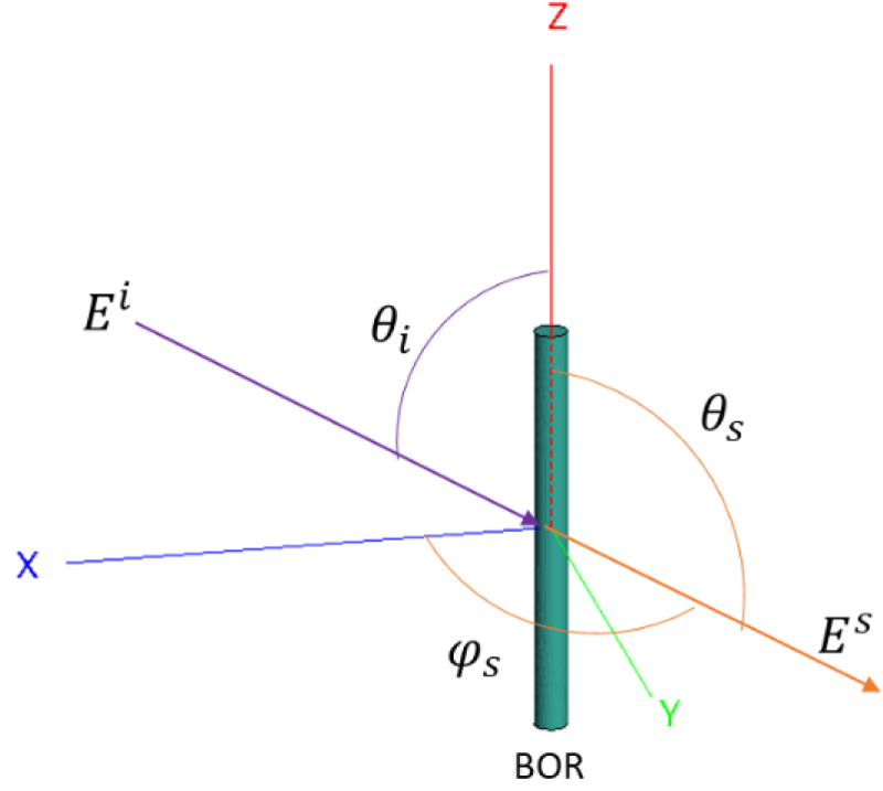
Figure 2: Cylinder scattering scene for spherical coordinates where $E^i$ is the incident electric field at ${\phi }_i=0{}^{\circ }$ and an arbitrary polar angle ${\theta }_i$. The variables $E^S$, ${\phi }_s$, and ${\theta }_s$ are the scattered electric field vector, radial scattering angle, and polar scattering angle, respectively.

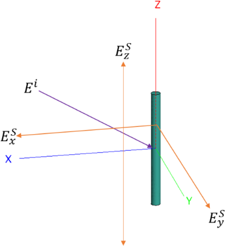
Figure 3: Cylinder scattering scene for Cartesian coordinates where $E^i$ is an incident electric field at ${\phi }_i=0{}^{\circ }$ and an arbitrary polar angle ${\theta }_i$. The variables $E_x^S$, $E_y^S$, and $E_z^S$ are the cardinal direction vectors in which the scattered fields shall be examined.

The complexity of near field scattering presents a vast dataset to validate against. For brevity, only the magnitude of the scattered fields is compared for both the scattered electric and magnetic fields in the principal component directions, r, $\theta$, $\phi$, x, y, and z. The cross polarized terms are neglected, and only bistatic scattering is considered. The results presented examine only scattering from both PEC and lossy dielectric cylinders, although the methodology can and has been evaluated for other shapes and material properties, e.g., spheres. For this analysis, the incident electric field will be 377 V/m, at a frequency of 3 GHz. Figures 2 and 3 shows the scene and scattering angles.

A. Far field evaluation

Presented in this section is validation of the scattered electric field calculation for the far field ($r>2D^2/\lambda$) using the generalized scattering definition for PEC BORs. Inherently, PEC BORs are of little value to vegetation scattering, but their evaluation is relevant in the total examination for the near field derivation. Table 1 lists the relevant statistics for the evaluation and validation. The first set of plots, Figs. 4–11, describe a far field comparison between BOR near field calculator and BOR scattering amplitude calculator at 100 m from BOR.

Table 1: PEC cylinder test cases for the validation of MoM with BOR, specifically cylinders

Cylinder Length	1$\lambda$, 3$\lambda$, 5$\lambda$, 10$\lambda$
Cylinder Radius	0.04$\lambda$
${\mathit{\theta }}_{\mathit{i}}$ [${}^{\mathbf{\circ }}$]	20${}^{\circ }$
${\mathit{ϵ}}_{\mathit{r}}$	PEC
Harmonics	10
Mesh Size	$\lambda$${}_m$/10
Range	100 m
E${}_{\mathrm{i}}$	377 V/m

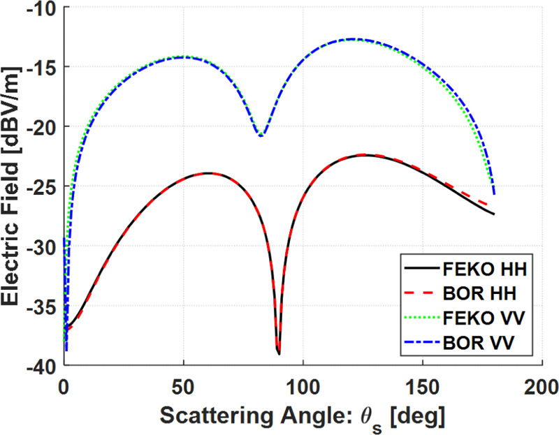
Figure 4: Magnitude of the bistatic electric field vs. ${\theta }_s$ on a PEC cylinder with a radius of 0.04$\lambda$, $L\mathrm{=}\mathrm{1}\mathit{}\lambda$, at ${\theta }_i=20{}^{\circ }$.

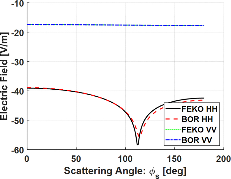
Figure 5: Magnitude of the bistatic electric field vs. ${\phi }_s$ on a PEC cylinder with a radius of 0.04$\lambda$, $L\mathrm{=}\mathrm{1}\mathit{}\lambda$, at ${\theta }_i=20{}^{\circ }$.

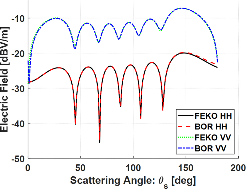
Figure 6: Magnitude of the bistatic electric field vs. ${\theta }_s$ on a PEC cylinder with a radius of 0.04$\lambda$, $L\mathrm{=}\mathrm{3}\mathit{}\lambda$, at ${\theta }_i=20{}^{\circ }$.

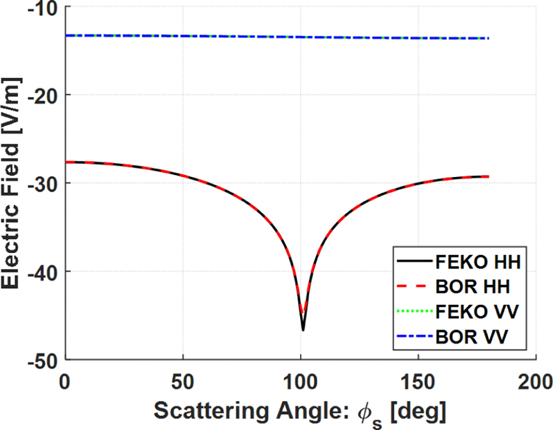
Figure 7: Magnitude of the bistatic electric field vs. ${\phi }_s$ on a PEC cylinder with a radius of 0.04$\lambda$, $L\mathrm{=}\mathrm{3}\mathit{}\lambda$, at ${\theta }_i=20{}^{\circ }$.

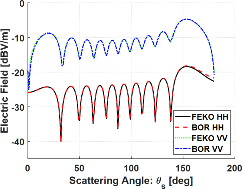
Figure 8: Magnitude of the bistatic electric field vs. ${\theta }_s$ on a PEC cylinder with a radius of 0.04$\lambda$, $L\mathrm{=}\mathrm{5}\mathit{}\lambda$, at ${\theta }_i=20{}^{\circ }$.

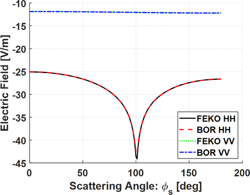
Figure 9: Magnitude of the bistatic electric field vs. ${\phi }_s$ on a PEC cylinder with a radius of 0.04$\lambda$, $L\mathrm{=}\mathrm{5}\mathit{}\lambda$, at ${\theta }_i=20{}^{\circ }$.

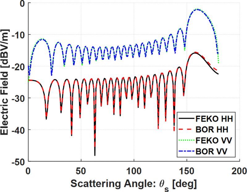
Figure 10: Magnitude of the bistatic electric field vs. ${\theta }_s$ on a PEC cylinder with a radius of 0.04$\lambda$, $L\mathrm{=}\mathrm{10}\mathit{}\lambda$, at${\theta }_i=20{}^{\circ }$.

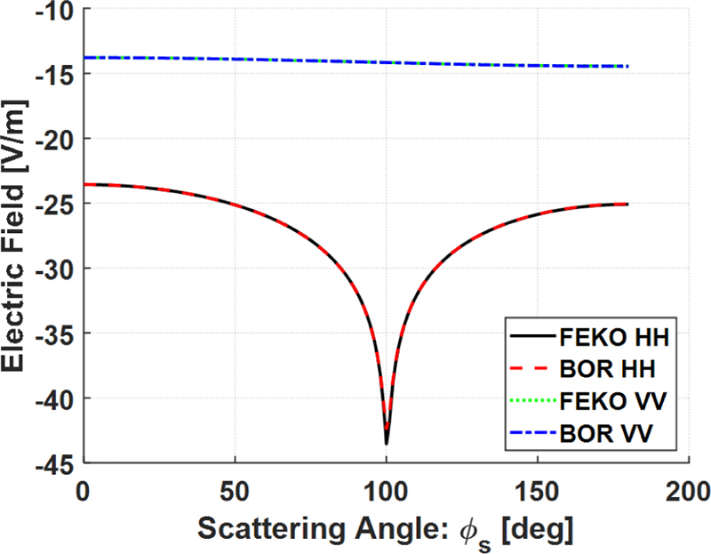
Figure 11: Magnitude of the bistatic electric field vs. ${\phi }_s$ on a PEC cylinder with a radius of 0.04$\lambda$, $L\mathrm{=}\mathrm{10}\mathit{}\lambda$, at${\theta }_i=20{}^{\circ }$.

B. Near field electric and magnetic field validation

Presented in this section is validation of the scattered electric and magnetic field calculation for the near field ($r<2D^2/\lambda$ and $kr\gg 1$) where $\lambda$ is the free space wavelength and $\lambda$${}_m$ is the material adjusted wavelength, using the generalized scattering definition. Table 2 lists the relevant statistics for the evaluation and validation. The plots shown in Figs. 12–22 compare BOR near field simulation and the FEKO© 3D MoM simulation. Note that because there exists a significant number of validation cases, the plots presented tend to capture an “entourage” of validation cases.

Table 2: Dielectric cylinder test cases for the validation of MoM with BOR, specifically cylinders

Cylinder Length	1$\lambda$, 5$\lambda$, 10$\lambda$
Cylinder Radius	0.04$\lambda$
Far Field Criterion	2$\lambda$, 50$\lambda$, 200$\lambda$
${\mathit{\theta }}_{\mathit{i}}$ [${}^{\mathbf{\circ }}$]	45${}^{\circ }$, 90${}^{\circ }$
${\mathit{ϵ}}_{\mathit{r}}$	18-j6
Harmonics	10
Mesh Size	$\lambda$${}_m$/10
Range	Varies
italicE${}_{\mathrm{i}}$	377 V/m

The first set of plots, Figs. 12–15, consider near field scattering from PEC cylinders with respect to $r_s$, ${\theta }_s$, and ${\phi }_s$ for both the electric and magnetic scattered fields. The second set of plots consider near field electric and magnetic field scattering from lossy dielectrics in Cartesian coordinates, i.e., scattering with respect to $x_s$,$y_s$, and $z_s$.

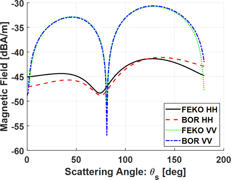
Figure 12: Magnitude of the bistatic magnetic field vs. ${\theta }_s$ on a PEC cylinder with a radius of 0.04$\lambda$, $L\mathrm{=}\mathrm{1}\mathit{}\lambda$, at ${\theta }_i=45{}^{\circ }$ at $r_s=0.1\mathrm{m}$.

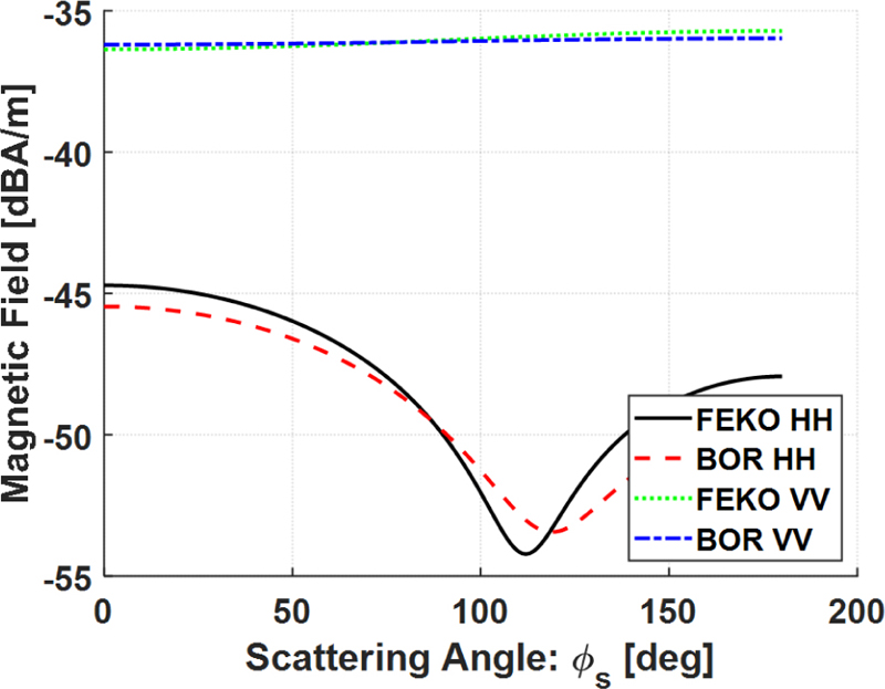
Figure 13: Magnitude of the bistatic magnetic field vs. ${\phi }_s$ for a PEC cylinder with a radius of 0.04$\lambda$, $L\mathrm{=}\mathrm{1}\mathit{}\lambda$, at ${\theta }_i=45{}^{\circ }$ at $r_s=0.1\mathrm{m}$.

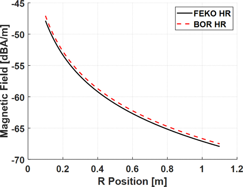
Figure 14: Magnitude of the bistatic magnetic field vs. $r_s$ with r polarized scattering for a PEC cylinder with a radius of 0.04$\lambda$, $L\mathrm{=}\mathrm{1}\mathit{}\lambda$, at ${\theta }_i=45{}^{\circ }$ at $r_s=0.1\mathrm{m}$.

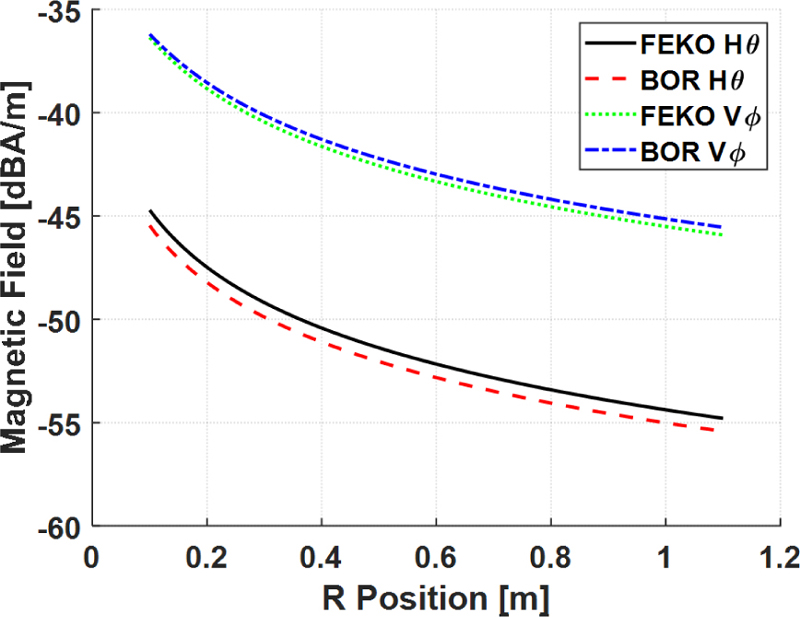
Figure 15: Magnitude of the bistatic magnetic field vs. $r_s$ with $\theta$ and $\phi$ polarized scattering for a PEC cylinder with a radius of 0.04$\lambda$, $L\mathrm{=}\mathrm{1}\mathit{}\lambda$, at ${\theta }_i=45{}^{\circ }$ at $r_s=0.1\mathrm{m}$.

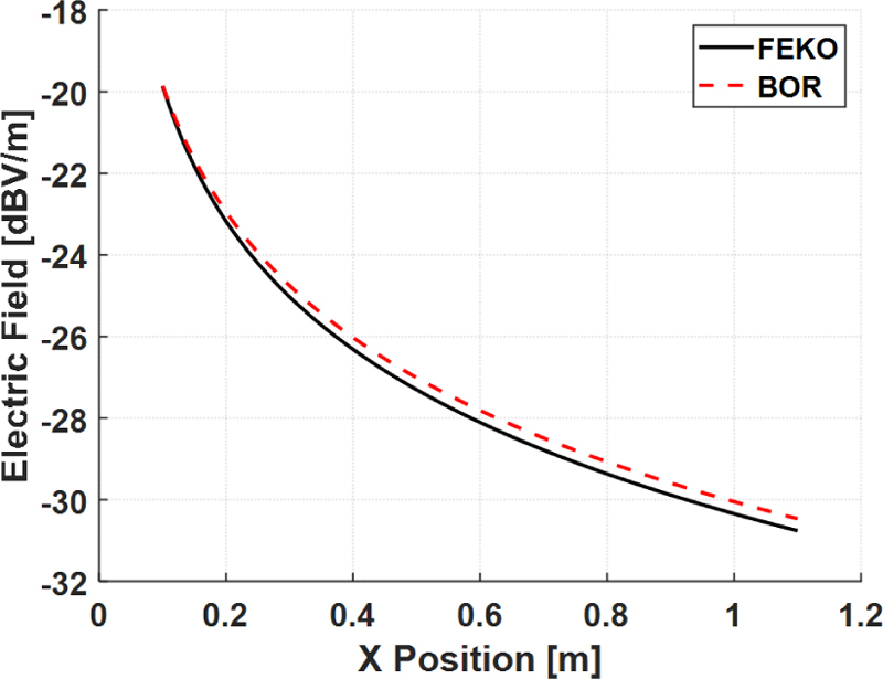
Figure 16: Magnitude of the bistatic electric field vs. $x_s$ for an H-polarized wave with $y$ polarized scattering on a dielectric cylinder with ${ϵ}_r=18-\mathrm{j6}$, radius of 0.04$\lambda$, $L\mathrm{=}\mathrm{1}\mathit{}\lambda$, at ${\theta }_i=90{}^{\circ }$, $y_s=0$ and $z_s=0$.

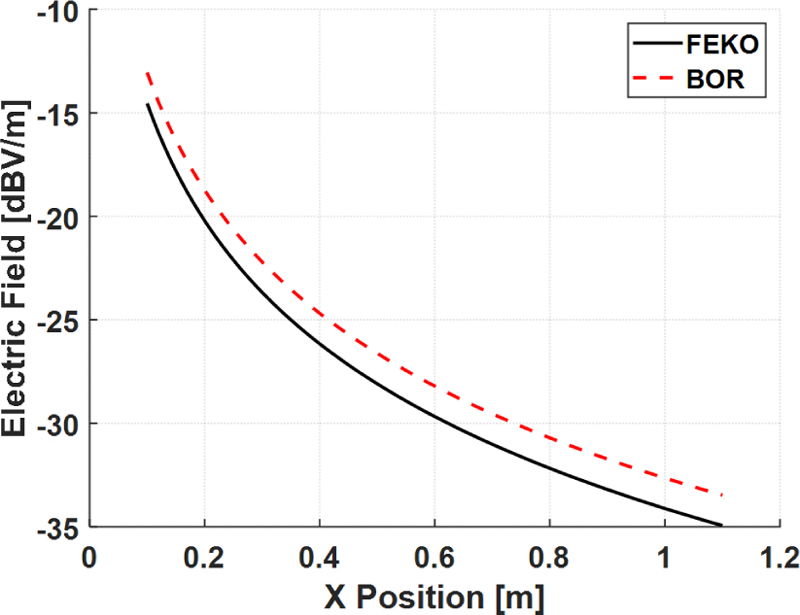
Figure 17: Magnitude of the bistatic electric field vs. $x_s$ for a V-polarized wave with x polarized scattering on a dielectric cylinder with ${ϵ}_r=18-\mathrm{j6}$, radius of 0.04$\lambda$, $L\mathrm{=}\mathrm{1}\mathit{}\lambda$, at ${\theta }_i=90{}^{\circ }$, $y_s=0$, and $z_s=0$.

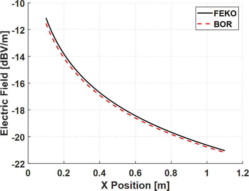
Figure 18: Magnitude of the bistatic electric field vs. $x_s$ for a V-polarized wave with $z$ polarized scattering on a dielectric cylinder with ${ϵ}_r=18-\mathrm{j6}$, radius of 0.04$\lambda$, $L\mathrm{=}\mathrm{1}\mathit{}\lambda$, at ${\theta }_i=90{}^{\circ }$, $y_s=0$, and $z_s=0$.

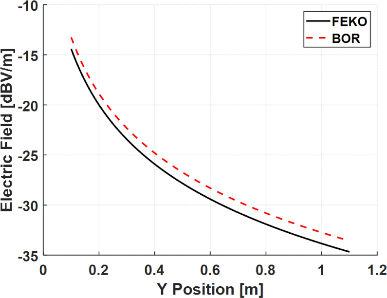
Figure 19: Magnitude of the bistatic electric field vs. $y_s$ for a V-polarized wave with $y$ polarized scattering on a dielectric cylinder with ${ϵ}_r=18-\mathrm{j6}$, radius of 0.04$\lambda$, $L\mathrm{=}\mathrm{1}\mathit{}\lambda$, at ${\theta }_i=90{}^{\circ }$, $x_s=0$, and $z_s=0$.

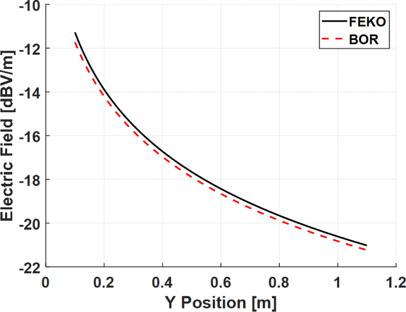
Figure 20: Magnitude of the bistatic electric field vs. $y_s$ for a V-polarized wave with $z$ polarized scattering on a dielectric cylinder with ${ϵ}_r=18-\mathrm{j6}$, radius of 0.04$\lambda$, $L\mathrm{=}\mathrm{1}\mathit{}\lambda$, at ${\theta }_i=90{}^{\circ }$, $x_s=0$, and $z_s=0$.

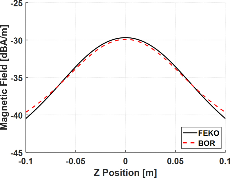
Figure 21: Magnitude of the bistatic magnetic field vs. $z_s$ for a V-polarized wave with y polarized scattering on a dielectric cylinder with ${ϵ}_r=18-\mathrm{j6}$, radius of 0.04$\lambda$, $L\mathrm{=}\mathrm{1}\mathit{}\lambda$, at ${\theta }_i=90{}^{\circ }$, $x_s=0$, and $y_s=0$.

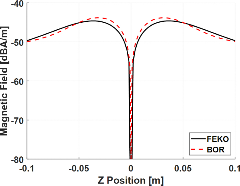
Figure 22: Magnitude of the bistatic magnetic field vs. $z_s$ for a H-polarized wave with x polarized scattering on a dielectric cylinder with ${ϵ}_r=18-\mathrm{j6}$, radius of 0.04$\lambda$, $L\mathrm{=}\mathrm{1}\mathit{}\lambda$, at ${\theta }_i=90{}^{\circ }$, $x_s=0$, and $y_s=0$.

The following plots will switch notation from XX, e.g., HH and VV, where XX represents an X-polarized scatter from an X-polarized incident field, to X$R$, X$\theta$, and X$\phi$, where $R$, $\theta$, and $\phi$ are the scattered field polarizations and X is the incident field polarization, either H or V. The change creates a more understandable representation of the three (3) orthogonal scattering polarizations for near field scattering.

Throughout part B, the validations between the 3D MoM and BOR-MoM show a greater degree of error than that of the far field comparison from part A. This error can be attributed to two factors. First, this implementation of BOR-MoM uses lower order basis functions resulting in lower order accuracy, especially in the near field where the fields are highly oscillatory and volatile, i.e., Gibb’s Phenomenon. Additionally, the error can be attributed to an inherent weakness of BOR-MoM, poor cross-polarization characterization of scatterers, e.g., HV and VH. This is a known phenomenon that occurs in BOR-MoM since the basis functions span only two principle directions whereas the 3D MoM basis functions span the three principle planes. Thus, the coherent summation of any cross polarized terms are neglected within this model resulting in a higher order of error. This does not affect the far field results as the cross-polarized terms are of significantly lower magnitude in the far field. Overall, this additional error can be considered inconsequential with regards to our applications; a discussion better served for afuture work.

V. VECTORIZATION OF BOR

BOR-MoM was selected as the method for evaluating axisymmetric objects due to its reduction of MoM from a 3D simulation to a 2-D simulation. This reduced the memory and computing requirements from $N_{3D}^2$ elements to approximately $n\cdot N_{1D}^2$ elements ($n\cdot N_{1D}^2$$<$$<$ $N_{\mathrm{3}\mathit{}D}^{\mathrm{2}}\mathrm{)}$, where n is the number of harmonics and $N$ is the number of segments due to the discretization. Based on previous simulation results, a maximum of 10 harmonics are required; thus, any object discretized into more than 10 segments will benefit in terms of speed and memory usage from BOR methodology.

A comparison of the FEKO© MoM solution and BOR-MoM solution with respect to computation time, number of elements, and peak memory usage is presented in Tables 3, 4 and 5. Additionally, Table 4 specifically compares the effects of vectorization on BOR-MoM implementation in MATLAB©. The comparisons use a dielectric cylinder with a dielectric constant of $ϵ=4$ and a radius of $\lambda$ at ${\theta }_i=45{}^{\circ }$ and ${\phi }_i=0{}^{\circ }$.

Table 3: BOR-MoM solution with respect to peak memory usage and computation time. Note that N represents the number of triangular elements and number of segments for the FEKO© and BOR meshes, respectively

	BOR-MoM Non-Vectorized
Length	N	Memory [GB]	Solver Time [s]
$\mathit{\lambda }$	122	8.7	207
3$\lambda$	202	10.6	481
6$\lambda$	322	10.6	1111
10$\lambda$	482	10.6	2399

Table 4: Vectorized BOR-MoM solution in MATLAB© with respect to peak memory usage and computation time. Note that N represents the number of triangular elements and number of segments for the FEKO© and BOR meshes, respectively

	BOR-MoM Vectorized
Length	N	Memory [GB]	Solver Time [s]
$\mathit{\lambda }$	123	22.1	29
3$\lambda$	203	22.7	78
6$\lambda$	323	24.1	196
10$\lambda$	483	26.4	469

Table 5: FEKO© 3D MoM solution with respect to peak memory usage and computation time. Note that N represents the number of triangular elements and number of segments for the FEKO© and BOR meshes, respectively

	FEKO© MoM
Length	N	Memory [GB]	Solver Time [s]
$\mathit{\lambda }$	4264	1.2	61
3$\lambda$	8328	4.7	238
6$\lambda$	14664	14.5	680
10$\lambda$	23320	35.9	2005

The test cases were run on a computer with an Intel i9-10900k CPU overclocked to 4.9 GHz all core, 64 GB of 3600 MHz DDR4 RAM, and a Samsung 970 Evo Plus NVMe SSD. Note that the computer had enough RAM such that a full in core solution was able to be run in FEKO©. If enough RAM is not available, an out of core solution must run - FEKO© writes data to and from the hard drive - which more than doubles computation time.

Overall, vectorization of BOR provided approximately a 10x speed but required additional memory usage. With regards to the 3D MoM, BOR provided an approximate 4x speed up. This implementation of BOR-MoM can be improved with regards to speed and memory usage through careful algorithm implementation in a coding language other than MATLAB©.

VI. CONCLUSION

Although scattering from BOR using MoM has been studied extensively, this paper provides derivation and application of an optimal and formally elegant mathematical formulation for near field scattering, for a particular implementation of BOR-MoM using a well-conditioned and numerically-stable basis function set. This elegant formulation should provide analysts with a direct computational encoding that minimizes required integrations. Although direct computational encodings have been derived previously for far field scattering, those derivations were not for the near fields.

The results of this study are a derivation of the generalized scattered field equations for BOR-MoM. Fields were derived for both the scattered electric and magnetic fields for all of space while accounting for the various coordinate transformations, Fourier series expansions, and basis function definitions.

The results were validated by comparison to the FEKO© 3D MoM solution near field calculations. The results showed great agreement between the different MoM implementations. The primary sources of error occurred in the reactive near field region of BOR. This error is likely due to the low order basis functions, triangular and rectangular, used within this implementation of BOR-MoM. This can be partially attributed to the occurrence of Gibb’s phenomenon within the Fourier series expansions and discretization along the generating arc. The sacrifice in accuracy due to low order basis functions, however, provides a benefit in computational speed for larger MoM problem sets. Overall, the error between the FEKO© MoM and BOR-MoM is an acceptable trade-off for the $>$4x speed increase that BOR-MoM provides, providing more tractable predictive simulations in practice.

With regards to this works impact on tree scattering analysis, examining the connections between branches and the interaction between multiple discrete scatterers is important for continued model verification, validation, and performance characterization. Further examination of these aspects, and associated discussion, however, defines separate and continuing studies in themselves, and thus not within the scope of this paper. Appropriately, such discussion is within the context of futurestudies.

ACKNOWLEDGMENT

This work is supported by the U.S. Military and funded through the U.S. Naval Research Laboratory Edison Memorial Graduate Training Program.

REFERENCES

[1] M. Kvicera, F. Pérez Fontán, J. Israel, and P. Pechac, “A new model for scattering from tree canopies based on physical optics and Multiple Scattering Theory,” IEEE Transactions on Antennas and Propagation, vol. 65, no. 4, pp. 1925-1933, Apr. 2017.

[2] A. Gendelman and A. Boag, “Fast multilevel physical optics algorithm for far- and near-field scattering analysis of very large targets,” in 2011 IEEE International Conference on Microwaves, Communications, Antennas and Electronic Systems (COMCAS 2011), Tel Aviv, Israel, pp. 1-2, 2011.

[3] M. Kvicera, F. Pérez-Fontán, J. Israel, and P. Pechac, “Modeling scattering from tree canopies for UAV scenarios,” in 2016 10th European Conference on Antennas and Propagation (EuCAP), Davos, Switzerland, pp. 1-3, 2016.

[4] M. Salim, S. Tan, R. D. De Roo, A. Colliander, and K. Sarabandi, “Passive and active multiple scattering of forests using radiative transfer theory with an iterative approach and cyclical corrections,” IEEE Transactions on Geoscience and Remote Sensing, vol. 60, pp. 1-16, 2022.

[5] Q. Zhao and R. H. Lang, “Scattering from tree branches using the Fresnel Double Scattering approximation,” in 2011 IEEE International Geoscience and Remote Sensing Symposium, Vancouver, BC, Canada, pp. 1040-1043, 2011.

[6] Y. Oh, Y. M. Jang, and K. Sarabandi, “Full-wave analysis of microwave scattering from short vegetation: An investigation on the effect of multiple scattering,” IEEE Trans. Geosci. Remote Sens., vol. 40, no. 11, pp. 2522-2526, Nov. 2002.

[7] W. Gu, L. Tsang, A. Colliander, and S. Yueh, “Hybrid method for full-wave simulations of forests at L-band,” IEEE Access, vol. 10, pp. 105898-105909, 2022.

[8] M. A. Karam, “A versatile scattering model for deciduous leaves,” in IGARSS ’98. Sensing and Managing the Environment. 1998 IEEE International Geoscience and Remote Sensing. Symposium Proceedings. (Cat. No.98CH36174), Seattle, WA, USA, pp. 2387-2389, 1998.

[9] A. W. Glisson and D. R. Wilton, “Simple and efficient numerical techniques for treating Bodies of Revolution,” Available https://apps.dtic.mil/sti/citations/ADA067361.

[10] S. Vitebskiy, K. Sturgess, and L. Carin, “Short-pulse plane-wave scattering from buried perfectly conducting Bodies of Revolution,” IEEE Transactions on Antennas and Propagation, vol. 44, no. 2, pp. 143-151, Feb. 1996.

[11] S. Vitebskiy and L. Carin, “Resonances of perfectly conducting wires and Bodies of Revolution buried in a lossy dispersive half-space,” IEEE Transactions on Antennas and Propagation, vol. 44, no. 12, pp. 1575-1583, Dec. 1996.

[12] N. Geng and L. Carin, “Wide-band electromagnetic scattering from a dielectric BOR buried in a layered lossy dispersive medium,” IEEE Transactions on Antennas and Propagation, vol. 47, no. 4, pp. 610-619, Apr. 1999.

[13] M. Andreasen, “Scattering from Bodies of Revolution,” IEEE Transactions on Antennas and Propagation, vol. 13, no. 2, pp. 303-310, Mar.1965.

[14] L. Carin, N. Geng, M. McClure, J. Sichina, and Lam Nguyen, “Ultra-wide-band synthetic-aperture radar for mine-field detection,” IEEE Antennas and Propagation Magazine, vol. 41, no. 1, pp. 18-33, Feb. 1999.

[15] N. Geng, D. R. Jackson, and L. Carin, “On the resonances of a dielectric BOR buried in a dispersive layered medium,” IEEE Transactions on Antennas and Propagation, vol. 47, no. 8, pp. 1305-1313, Aug. 1999.

[16] J. He, T. Yu, N. Geng, and L. Carin, “Method of moments analysis of electromagnetic scattering from a general three-dimensional dielectric target embedded in a multilayered medium,” Radio Science, vol. 35, no. 2, pp. 305-313, Mar.-Apr. 2000.

[17] J. R. Mautz and R. F. Harrington, “Radiation and scattering from Bodies of Revolution,” Applied Scientific Research, vol. 20, pp. 405-435, 1969.

[18] T.-K. Wu and L. L. Tsai, “Scattering from arbitrarily-shaped lossy dielectric Bodies of Revolution,” Radio Science, vol. 12, pp. 709-718, 1977.

[19] G. Pisharody and D. S. Weile, “Electromagnetic scattering from a homogeneous material body using time domain integral equations and bandlimited extrapolation,” in IEEE Antennas and Propagation Society International Symposium. Digest. Held in conjunction with: USNC/CNC/URSI North American Radio Sci. Meeting (Cat. No.03CH37450), Columbus, OH, USA, vol. 3, pp. 567-570, 2003.

[20] J. R. Mautz and R. F. Harrington, “Electromagnetic scattering from a homogeneous Body of Revolution,” Technical Report, Defense Technical Information Center, Nov. 1977.

[21] P. de Matthaeis and R. H. Lang, “Comparison of surface and volume currents models for electromagnetic scattering from finite dielectric cylinders,” IEEE Transactions on Antennas and Propagation, vol. 57, no. 7, pp. 2216-2220, July 2009.

[22] P. de Matthaeis and R. H. Lang, “Numerical calculations of microwave scattering from dielectric structures used in vegetation models,” Ph.D. thesis, ECE Department, The George Washington University, Washington, DC, 2006.

[23] A. Glisson and C. Butler, “Analysis of a wire antenna in the presence of a Body of Revolution,” IEEE Transactions on Antennas and Propagation, vol. 28, no. 5, pp. 604-609, Sep. 1980.

[24] S. H. Yueh, J. A. Kong, J. K. Jao, R. T. Shin, and T. Le Toan, “Branching model for vegetation,” IEEE Transactions on Geoscience and Remote Sensing, vol. 30, no. 2, pp. 390-402, Mar. 1992.

[25] T. Su, L. Du, and R. Chen, “Electromagnetic scattering for multiple PEC Bodies of Revolution using equivalence principle algorithm,” IEEE Transactions on Antennas and Propagation, vol. 62, no. 5, pp. 2736-2744, May 2014.

[26] M. Jiang, Y. Li, Z. Rong, L. Lei, Y. Chen, and J. Hu, “Fast solving scattering from multiple Bodies of Revolution with arbitrarily metallic-dielectric combinations,” IEEE Transactions on Antennas and Propagation, vol. 67, no. 7, pp. 4748-4755, July 2019.

[27] H. Huang, L. Tsang, A. Colliander, and S. Yueh, “Full wave simulations of vegetation/trees using 3D vector cylindrical wave expansions in Foldy-Lax multiple scattering equations,” in 2019 IEEE International Conference on Computational Electromagnetics (ICCEM), Shanghai, China, pp. 1-3, 2019.

[28] H. Huang, L. Tsang, E. G. Njoku, A. Colliander, K.-H. Ding, and T.-H. Liao, “Hybrid method combining generalized T matrix of single objects and Foldy-Lax equations in NMM3D microwave scattering in vegetation,” in 2017 Progress in Electromagnetics Research Symposium - Fall (PIERS - FALL), Singapore, pp. 3016-3023, 2017.

[29] H. Huang, L. Tsang, A. Colliander, R. Shah, X. Xu, and S. Yueh, “Multiple scattering of waves by complex objects using hybrid method of T-Matrix and Foldy-Lax equations using vector spherical waves and vector spheroidal waves,” Progress in Electromagnetics Research, vol. 168, pp. 87-111, 2020.

[30] H. Huang, L. Tsang, E. G. Njoku, A. Colliander, T.-H. Liao and K.-H. Ding, “Propagation and scattering by a layer of randomly distributed dielectric cylinders using Monte Carlo simulations of 3D Maxwell equations with applications in microwave interactions with vegetation,” IEEE Access, vol. 5, pp. 11985-12003, 2017.

[31] M. Kvicera, F. Pérez Fontán, J. Israel, and P. Pechac, “A new model for scattering from tree canopies based on physical optics and Multiple Scattering Theory,” IEEE Transactions on Antennas and Propagation, vol. 65, no. 4, pp. 1925-1933, Apr. 2017.

BIOGRAPHIES

Edward C. Michaelchuck Jr. is currently pursuing a Ph.D. in electrical engineering with a focus in applied electromagnetics at The George Washington University, Washington D.C., USA. He received a M.S. degree in electrical engineering with a concentration in applied electromagnetics from George Washington University, Washington D.C., USA, in January 2021. He received a B.S. in mechanical engineering from Rowan University, Glassboro, NJ, USA, in May 2017.

With regards to his career, he acted as a research assistant for Dr. Parth Bhavsar at Rowan University from 2015 to 2017 studying traffic monitoring systems. He interned at PSE&G Salem Nuclear Power plant in 2016. Currently, he is at the Signature Technology Office, Code 5009, at the U.S. Naval Research Laboratory, Washington, D.C., USA, since August 2017. His expertise includes multispectral signature characterization, computational electromagnetics, RF material measurements, and machine design.

Samuel G. Lambrakos received the Ph.D. degree in Physics from the Polytechnic Institute of New York University in 1983.

He is currently a Research Physicist at the U.S. Naval Research Laboratory, Code 8113, Washington, D.C., where he has been for over 35 years. His expertise is computational physics in general and has many publications, patents and awards. His recent studies concern computational materials physics and inverse spectral analysis.

William O. Coburn received his B.S. in Physics from Virginia Polytechnic Institute in 1984. He received an MSEE in Electro Physics in 1991 and Doctor of Science in Electromagnetic Engineering from The George Washington University (GWU) in 2005. His dissertation research was in traveling wave antenna design.

He has 38 years’ experience as an Electronics Engineer at the Army Research Laboratory (formerly the Harry Diamond Laboratories) primarily in the area of CEM for EMP coupling/hardening, HPM, target signatures and antennas. He retired in 2019 from the RF Electronics Division of the Sensors and Electron Devices Directorate applying CEM tools for antenna design and EM analysis.

He is a Fellow of the Applied Computational EM Society (ACES) and served on the ACES Board of Directors. He is a Member of the USNC-URSI, Commission A and B (2010), Sigma Xi and an Adjunct Professor at the Catholic University of America and GWU. Coburn has authored or coauthored over 100 publications and four patents.

APPENDIX I: SPHERICAL COORDINATES

The scattering definition using equivalent sources is:

	${\mathbf{E}}^s(\mathbf{r})$	$=-j\omega {\mu }_0{\displaystyle \oint {\underset{¯}{\mathbf{G}}}^0(\mathbf{r},{\mathbf{r}}^{\prime })\cdot {\mathbf{J}}_s\left({\mathbf{r}}^{\prime }\right)\mathit{d}{S}^{\prime }}+$
		$\mathrm{\hspace{1em}}-{\displaystyle \oint {\underset{¯}{\mathbf{K}}}^0(\mathbf{r},{\mathbf{r}}^{\prime })\cdot {\mathbf{M}}_s\left({\mathbf{r}}^{\prime }\right)\mathit{d}{S}^{\prime }},$		(50)

	${\mathbf{H}}^s(\mathbf{r})$	$={\displaystyle \oint {\underset{¯}{\mathbf{K}}}^0(\mathbf{r},{\mathbf{r}}^{\prime })\cdot J_s\left({\mathbf{r}}^{\prime }\right)\mathit{d}{S}^{\prime }}+$
		$\mathrm{\hspace{1em}}-j\omega {ϵ}_0{\displaystyle \oint {\underset{¯}{\mathbf{G}}}^0(\mathbf{r},{\mathbf{r}}^{\prime })\cdot {\mathbf{M}}_s\left({\mathbf{r}}^{\prime }\right)\mathit{d}{S}^{\prime }}.$		(51)

Following the analysis from section III, the integration along the generating arc, $l$, over a single segment for a single harmonic becomes:

	${\mathbf{E}}_{1,n,r,m}^s=\mathrm{\Delta }{l}_{m,k}{\rho }_m{\displaystyle \underset{0}{\overset{2\pi }{\int }}}{g}^0(\mathbf{r},{\mathbf{r}}_{\mathbf{m}})F_{r,n,m}\left(J_{n,m}\right)e^{jn{\phi }^{\prime }}\mathit{d}{\phi }^{\prime }\widehat{\mathbf{r}},$		(52)
	${\mathbf{E}}_{1,n,\phi ,m}^s=\mathrm{\Delta }{l}_{m,k}{\rho }_m{\displaystyle \underset{0}{\overset{2\pi }{\int }}}{g}^0(\mathbf{r},{\mathbf{r}}_{\mathbf{m}})F_{\phi ,n,m}\left(J_{n,m}\right)e^{jn{\phi }^{\prime }}\mathit{d}{\phi }^{\prime }\widehat{\mathit{\phi }},$		(53)
	${\mathbf{E}}_{1,n,\theta ,m}^s=\mathrm{\Delta }{l}_{m,k}{\rho }_m{\displaystyle {\int }^{2\pi }}{g}^0(\mathbf{r},{\mathbf{r}}_{\mathbf{m}})F_{\theta ,n,m}\left(J_{n,m}\right)e^{jn{\phi }^{\prime }}\mathit{d}{\phi }^{\prime }\widehat{\mathit{\theta }},$		(54)
	${\mathbf{E}}_{2,r,n,m}^s=\mathrm{\Delta }{l}_{m,k}{\rho }_m{\displaystyle \underset{0}{\overset{2\pi }{\int }}}{D}_{r,n,m}\left(M_{n,m}\right)e^{jn{\phi }^{\prime }}\mathit{d}{\phi }^{\prime }\widehat{\mathbf{r}},$		(55)
	${\mathbf{E}}_{2,\theta ,n,m}^s=\mathrm{\Delta }{l}_{m,k}{\rho }_m{\displaystyle \underset{0}{\overset{2\pi }{\int }}}{D}_{\theta ,n,m}\left(M_{n,m}\right)e^{jn{\phi }^{\prime }}\mathit{d}{\phi }^{\prime }\widehat{\mathit{\theta }},$		(56)
	${\mathbf{E}}_{2,\phi ,n,m}^s=\mathrm{\Delta }{l}_{m,k}{\rho }_m{\displaystyle \underset{\phi ,n,m}{\overset{2\pi }{\int }}}\left(M_{n,m}\right)e^{jn{\phi }^{\prime }}\mathit{d}{\phi }^{\prime }\widehat{\mathit{\phi }}.$		(57)

These equations require the expansion of $F_{r,n,m}$,$F_{\phi ,n,m}$, $F_{\theta ,n,m}$, $D_{r,n,m}$, $D_{\theta ,n,m}$, and $D_{\phi ,n,m}$ terms. Due to the length of the derivation for these terms, only the final results will be listed below. The $F$ terms are:

	$F_r\left({\mathit{J}}_{s,n}\right)=\left(\begin{array}{c}\hfill A_1{J}_{\tau ,n}{C}_1+A_1{J}_{\phi ,n}{C}_2+\hfill \\ \hfill +A_2{J}_{\tau ,n}\sin \theta \sin {\psi }^{\prime }\cos \left(\phi -{\phi }^{\prime }\right)+\hfill \\ \hfill +A_2{J}_{\tau ,n}\cos \theta \cos {\psi }^{\prime }+\hfill \\ \hfill +A_2{J}_{\phi ,n}\sin \theta \sin \left(\phi -{\phi }^{\prime }\right)\hfill \end{array}\right),$		(58)
	$F_{\phi }\left({\mathit{J}}_{s,n}\right)=A_2{J}_{\tau ,n}\sin {\psi }^{\prime }\sin \left({\phi }^{\prime }-\phi \right)+$
	$\mathrm{\hspace{1em}\hspace{1em}}\mathit{\hspace{1em}\hspace{1em}}+A_2{J}_{\phi ,n}\cos \left(\phi -{\phi }^{\prime }\right),$		(59)
	$F_{\theta }\left(J_{s,n}\right)=A_2{J}_{\tau ,n}\cos \theta \sin {\psi }^{\prime }\cos \left(\phi -{\phi }^{\prime }\right)+$
	$\mathrm{\hspace{1em}\hspace{1em}}\mathit{\hspace{1em}\hspace{1em}}-A_2{J}_{\tau ,n}\sin \theta \cos {\psi }^{\prime }+$
	$\mathrm{\hspace{1em}\hspace{1em}}\mathit{\hspace{1em}\hspace{1em}}+A_2{J}_{\phi ,n}\cos \theta \sin \left(\phi -{\phi }^{\prime }\right),$		(60)

where the A terms and C terms are:

	$A_1$	$={\displaystyle \frac{3}{k_0^2{R}^2}}+{\displaystyle \frac{3j}{k_{0}R}}-1,$		(61)
	$A_2$	$=1-{\displaystyle \frac{j}{k_{0}R}}-{\displaystyle \frac{1}{k_0^2{R}^2}},$		(62)
	$C_1$	$=\sin \theta \sin {\psi }^{\prime }\cos \left(\phi -{\phi }^{\prime }\right)+\cos \theta \cos {\psi }^{\prime },$		(63)
	$C_2$	$=\sin \theta \sin \left(\phi -{\phi }^{\prime }\right),$		(64)

and R in spherical coordinates is:

$$\begin{array}{c}\hfill R=\sqrt{\begin{array}{c}\hfill r^2+r^{\prime }{}^2+\hfill \\ \hfill -2r{r}^{\prime }\sin \theta \sin {\theta }^{\prime }\cos \left(\phi -{\phi }^{\prime }\right)+\hfill \\ \hfill -2r{r}^{\prime }\cos \theta \cos {\theta }^{\prime }\hfill \end{array}}.\hfill \end{array}$$

(65)

The $D$ terms are derived as:

$$\begin{array}{c}\hfill D_r\left({\mathit{M}}_n\right)=\begin{array}{c}\hfill {\mathit{M}}_{\tau ,n}\left({\mathit{l}}^{\prime }\right)\frac{1}{r}\frac{dg}{d\theta }\sin {\psi }^{\prime }\sin \left({\phi }^{\prime }-\phi \right)+\hfill \\ \hfill -\frac{{\mathit{M}}_{\tau ,n}\left({\mathit{l}}^{\prime }\right)}{r\sin \theta }\frac{dg}{d\phi }\cos \theta \sin {\psi }^{\prime }\cos \left(\phi -{\phi }^{\prime }\right)+\hfill \\ \hfill +\frac{{\mathit{M}}_{\tau ,n}\left({\mathit{l}}^{\prime }\right)}{r\sin \theta }\frac{dg}{d\phi }\sin \theta \cos {\psi }^{\prime }+\hfill \\ \hfill +{\mathit{M}}_{\phi ,n}\left({\mathit{l}}^{\prime }\right)\frac{1}{r}\frac{dg}{d\theta }\cos \left(\phi -{\phi }^{\prime }\right)+\hfill \\ \hfill -{\mathit{M}}_{\phi ,n}\left({\mathit{l}}^{\prime }\right)\frac{1}{r\sin \theta }\frac{dg}{d\phi }\cos \theta \sin \left(\phi -{\phi }^{\prime }\right)\hfill \end{array},\hfill \end{array}$$

(66)

$$\begin{array}{c}\hfill D_{\theta }\left({\mathit{M}}_n\right)=\begin{array}{c}\hfill -{\mathit{M}}_{\tau ,n}\left({\mathit{l}}^{\prime }\right)\frac{dg}{dr}\sin {\psi }^{\prime }\sin \left({\phi }^{\prime }-\phi \right)+\hfill \\ \hfill +{\mathit{M}}_{\tau ,n}\left({\mathit{l}}^{\prime }\right)\frac{1}{r\sin \theta }\frac{dg}{d\phi }\sin \theta \sin {\psi }^{\prime }\cos \left(\phi -{\phi }^{\prime }\right)+\hfill \\ \hfill +{\mathit{M}}_{\tau ,n}\left({\mathit{l}}^{\prime }\right)\frac{1}{r\sin \theta }\frac{dg}{d\phi }\cos \theta \cos {\psi }^{\prime }+\hfill \\ \hfill -{\mathit{M}}_{\phi ,n}\left({\mathit{l}}^{\prime }\right)\frac{dg}{dr}\cos \left(\phi -{\phi }^{\prime }\right)+\hfill \\ \hfill +{\mathit{M}}_{\phi ,n}\left({\mathit{l}}^{\prime }\right)\frac{1}{r\sin \theta }\frac{dg}{d\phi }\sin \theta \sin \left(\phi -{\phi }^{\prime }\right)\hfill \end{array},\hfill \end{array}$$

(67)

$$\begin{array}{c}\hfill D_{\phi }\left({\mathit{M}}_n\right)=\begin{array}{c}\hfill {\mathit{M}}_{\tau ,n}\left({\mathit{l}}^{\prime }\right)\frac{dg}{dr}\cos \theta \sin {\psi }^{\prime }\cos \left(\phi -{\phi }^{\prime }\right)+\hfill \\ \hfill -{\mathit{M}}_{\tau ,n}\left({\mathit{l}}^{\prime }\right)\frac{dg}{dr}\sin \theta \cos {\psi }^{\prime }+\hfill \\ \hfill -{\mathit{M}}_{\tau ,n}\left({\mathit{l}}^{\prime }\right)\frac{1}{r}\frac{dg}{d\theta }\sin \theta \sin {\psi }^{\prime }\cos \left(\phi -{\phi }^{\prime }\right)+\hfill \\ \hfill -{\mathit{M}}_{\tau ,n}\left({\mathit{l}}^{\prime }\right)\frac{1}{r}\frac{dg}{d\theta }\cos \theta \cos {\psi }^{\prime }+\hfill \\ \hfill {\mathit{M}}_{\phi ,n}\left({\mathit{l}}^{\prime }\right)\frac{dg}{dr}\cos \theta \sin \left(\phi -{\phi }^{\prime }\right)+\hfill \\ \hfill -{\mathit{M}}_{\phi ,n}\left({\mathit{l}}^{\prime }\right)\frac{1}{r}\frac{dg}{d\theta }\sin \theta \sin \left(\phi -{\phi }^{\prime }\right)\hfill \end{array},\hfill \end{array}$$

(68)

where:

	${\displaystyle \frac{dg}{dr}}$	$=\left({\displaystyle \genfrac{}{}{0pt}{}{r-r^{\prime }\sin \theta \sin {\theta }^{\prime }\cos \left(\phi -{\phi }^{\prime }\right)+}{-r^{\prime }\cos \theta \cos {\theta }^{\prime }}}\right){\displaystyle \frac{e^{-j{k}_{0}R}}{4\pi R}}\left({\displaystyle \frac{-jk}{R}}-{\displaystyle \frac{1}{\sqrt{R}}}\right),$		(69)
	${\displaystyle \frac{dg}{d\theta }}$	$=\left({\displaystyle \genfrac{}{}{0pt}{}{r{r}^{\prime }\cos {\theta }^{\prime }\sin \theta +}{-r{r}^{\prime }\sin {\theta }^{\prime }\cos \left(\phi -{\phi }^{\prime }\right)\cos \theta }}\right){\displaystyle \frac{e^{-j{k}_{0}R}}{4\pi R}}\left({\displaystyle \frac{-jk}{R}}-{\displaystyle \frac{1}{\sqrt{R}}}\right),$		(70)
	${\displaystyle \frac{dg}{d\phi }}$	$=r{r}^{\prime }\sin \theta \sin {\theta }^{\prime }\sin \left(\phi -{\phi }^{\prime }\right){\displaystyle \frac{e^{-j{k}_{0}R}}{4\pi R}}\left({\displaystyle \frac{-jk}{R}}-{\displaystyle \frac{1}{\sqrt{R}}}\right).$		(71)

APPENDIX II: CARTESIAN COORDINATES

Similar to Appendix I, the scattered electric and magnetic fields can be expanded in the Cartesian coordinate system. The electric field (${\mathit{E}}_{1,n,m,x}^s)$ as a function of the electric surface currents for a single harmonic over a single segment is:

	${\mathit{E}}_{1,n,m,x}^s=\mathrm{\Delta }{l}_{m,k}{\rho }_m{\displaystyle \int g^0(\mathit{r},{\mathit{r}}_{\mathit{m}})F_{x,J}\left(J_{n,m}\right)e^{jn{\phi }^{\prime }}\mathit{d}{\phi }^{\prime }\widehat{\mathit{x}}},$		(72)
	${\mathit{E}}_{1,n,m,y}^s=\mathrm{\Delta }{l}_{m,k}{\rho }_m{\displaystyle \int g^0(\mathit{r},{\mathit{r}}_{\mathit{m}})F_{y,J}\left(J_{n,m}\right)e^{jn{\phi }^{\prime }}\mathit{d}{\phi }^{\prime }\widehat{\mathit{y}}},$		(73)
	${\mathit{E}}_{1,n,m,z}^s=\mathrm{\Delta }{l}_{m,k}{\rho }_m{\displaystyle \int g^0(\mathit{r},{\mathit{r}}_{\mathit{m}})F_{z,J}\left(J_{n,m}\right)e^{jn{\phi }^{\prime }}\mathit{d}{\phi }^{\prime }\widehat{\mathbf{z}}},$		(74)

where:

	$F_x\left(J_{n,m}\right)$	$=A_1{C}_1{R}_x{J}_{\tau ,n}+A_1{C}_2{R}_x{J}_{\phi ,n}+$
		$\mathrm{\hspace{1em}}+A_2\sin {\psi }^{\prime }\cos {\phi }^{\prime }{J}_{\tau ,n}-A_2\sin {\phi }^{\prime }{J}_{\phi ,n},$		(75)
	$F_y\left(J_{n,m}\right)$	$=A_1{C}_1{R}_y{J}_{\tau ,n}+A_1{C}_2{R}_y{J}_{\phi ,n}+$
		$\mathrm{\hspace{1em}}+A_2\sin {\psi }^{\prime }\sin {\phi }^{\prime }{J}_{\tau ,n}+A_2\cos {\phi }^{\prime }{J}_{\phi ,n},$		(76)
	$F_z\left(J_{n,m}\right)$	$=A_1{C}_1{R}_z{J}_{\tau ,n}+A_1{C}_2{R}_z{J}_{\phi ,n}+$
		$\mathrm{\hspace{1em}}+A_2\cos {\psi }^{\prime }{J}_{\tau ,n}.$		(77)

The electric field (${\mathit{E}}_{2,n,m,x}^s)$ as a function of the fictitious magnetic surface currents for a single harmonic over a single segment is:

	${\mathit{E}}_{2,x,n,m}^s$	$={\displaystyle \underset{S}{\int }}{D}_x\left(M_{n,m}\right)e^{jn{\phi }^{\prime }}\mathit{d}{S}^{\prime }\widehat{\mathit{x}},$		(78)
	${\mathit{E}}_{2,y,n,m}^s$	$={\displaystyle \underset{S}{\int }}{D}_y\left(M_{n,m}\right)e^{jn{\phi }^{\prime }}\mathit{d}{S}^{\prime }\widehat{\mathit{y}},$		(79)
	${\mathit{E}}_{2,z,n,m}^s$	$={\displaystyle \underset{S}{\int }}{D}_z\left(M_{n,m}\right)e^{jn{\phi }^{\prime }}\mathit{d}{S}^{\prime }\widehat{\mathit{z}},$		(80)

where:

	$D_x$	$={\mathit{M}}_{\tau ,n}\left({\mathit{l}}^{\prime }\right){\displaystyle \frac{dg}{dy}}\cos {\psi }^{\prime }+$
		$\mathrm{\hspace{1em}}-{\mathit{M}}_{\tau ,n}\left({\mathit{l}}^{\prime }\right){\displaystyle \frac{dg}{dz}}\sin {\psi }^{\prime }\sin {\phi }^{\prime }+$
		$\mathrm{\hspace{1em}}-{\mathit{M}}_{\phi ,n}\left({\mathit{l}}^{\prime }\right){\displaystyle \frac{dg}{dz}}\cos {\phi }^{\prime },$		(81)
	$D_y$	$=-{\mathit{M}}_{\tau ,n}\left({\mathit{l}}^{\prime }\right){\displaystyle \frac{dg}{dx}}\cos {\psi }^{\prime }+$
		$\mathrm{\hspace{1em}}-{\mathit{M}}_{\tau ,n}\left({\mathit{l}}^{\prime }\right){\displaystyle \frac{dg}{dz}}\sin {\phi }^{\prime }+$
		$\mathrm{\hspace{1em}}-{\mathit{M}}_{\phi ,n}\left({\mathit{l}}^{\prime }\right){\displaystyle \frac{dg}{dz}}\sin {\phi }^{\prime },$		(82)
	$D_z=$	${\mathit{M}}_{\tau ,n}\left({\mathit{l}}^{\prime }\right){\displaystyle \frac{dg}{dx}}\sin {\psi }^{\prime }\sin {\phi }^{\prime }+$
		$+{\mathit{M}}_{\tau ,n}\left({\mathit{l}}^{\prime }\right){\displaystyle \frac{dg}{dy}}\sin {\phi }^{\prime }+$
		$+{\mathit{M}}_{\phi ,n}\left({\mathit{l}}^{\prime }\right){\displaystyle \frac{dg}{dx}}\cos {\phi }^{\prime }+$
		$+{\mathit{M}}_{\phi ,n}\left({\mathit{l}}^{\prime }\right){\displaystyle \frac{dg}{dy}}\sin {\phi }^{\prime },$		(83)

and the Green’s functions derivatives are:

	${\displaystyle \frac{dg}{dx}}$	$={\displaystyle \frac{\left(x-x^{\prime }\right)e^{-j{k}_{0}R}}{4\pi R}}\left({\displaystyle \frac{-jk}{R}}-{\displaystyle \frac{1}{\sqrt{R}}}\right),$		(84)
	${\displaystyle \frac{dg}{dy}}$	$={\displaystyle \frac{\left(y-y^{\prime }\right)e^{-j{k}_{0}R}}{4\pi R}}\left({\displaystyle \frac{-jk}{R}}-{\displaystyle \frac{1}{\sqrt{R}}}\right),$		(85)
	${\displaystyle \frac{dg}{dz}}$	$={\displaystyle \frac{\left(z-z^{\prime }\right)e^{-j{k}_{0}R}}{4\pi R}}\left({\displaystyle \frac{-jk}{R}}-{\displaystyle \frac{1}{\sqrt{R}}}\right).$		(86)

ACES JOURNAL, Vol. 39, No. 5, 376–389
doi: 10.13052/2024.ACES.J.390501
© 2024 River Publishers