Efficient MAPoD via Least Angle Regression based Polynomial Chaos Expansion Metamodel for Eddy Current NDT
Yang Bao, Jiahao Qiu, Praveen Gurrala, and Jiming Song
1College of Electronic and Optical Engineering
Nanjing University of Posts and Telecommunications, Nanjing, Jiangsu 210023, China
brianbao@njupt.edu.cn
2Micron Technology, Inc.
Boise, ID 83707, USA
3Department of Electrical and Computer Engineering
Iowa State University, Ames, IA 50011, USA
Submitted On: February 12, 2024; Accepted On: July 2, 2024
ABSTRACT
In this article, a metamodeling approach based on non-intrusive polynomial chaos expansion (PCE) with least angle regression (LAR) method is used in boundary element analysis for a model-assisted probability of detection (MAPoD) study of eddy current nondestructive testing (NDT) systems. The LAR-PCE metamodel represents the NDT system model responses by a set of coefficients with the polynomial basis functions in lieu of pure kernel degeneration accelerated boundary element method (KD-BEM) based physical model. Both the computational accuracy and efficiency of the LAR-PCE metamodel over the ordinary least squares (OLS) based PCE metamodel are demonstrated by testing the 3D eddy current NDT benchmarks with different system setups, flaw lengths and widths. The simulation results show two digits accuracy of the PoD metrics compared with the ones achieved by the KD-BEM based physical model as the benchmark. The LAR-PCE metamodel has remarkable improvements in computational efficiency over the OLS-PCE metamodel and accelerates the MAPoD study.
Index Terms: Boundary element analysis, eddy current nondestructive testing (NDT), meta learning, model-assisted probability of detection (MAPoD), polynomial chaos expansions with least angle regression (LAR-PCE).
I. INTRODUCTION
Eddy current nondestructive testing (NDT) plays a critical role in testing for material damage and discontinuities (flaws) in components and in assessing the risk of component failure. Because it provides high sensitivity to small defects without needing to make direct contact with inspection samples, it has gained popularity in many industries such as aerospace, nuclear, railways, and special equipment [1]. In general, components need to be replaced if they have flaws whose sizes exceed a threshold value that is considered harmless [2]. Therefore, it is very important for NDT inspections to estimate the flaw sizes precisely. Imperfect estimation is primarily caused by measurement uncertainties (such as environmental conditions, human factors and protective clothing). Multiple output responses obtained repeatedly using the same (nominal) test parameters and conditions may vary significantly because of measurement uncertainties, thus impacting the reliability of the NDT system [3]. To quantify the reliability of NDT systems, the notion of probability of detection (PoD) is introduced [4]. PoD represents the probability of detecting a flaw as a function of flaw size. PoD study is applied to both eddy current and ultrasonic NDT by evaluating the presence of a flaw with the impedance variations and reflected signals, respectively. It is also applied to evaluate wall thinning due to backwall echo [5].
PoD assessments typically require performing a large number of tests accurately to quantify the impact of all uncertainties. It is challenging to perform a large number of measurements due to time and labor costs. Thus, accurate theoretical and numerical simulation models, which have been validated by experiment, are replacing physical measurements partly or entirely to get the required data for PoD analysis. This approach is called model assisted PoD (MAPoD) [6]. The simulation models used in the above process need to be accurate and efficient to ensure MAPoD analysis remains accurate without requiring large amounts of computer resources. Several simulation models have been proposed as forward solvers in eddy current NDT [7–10]. Generally, these solvers can be categorized into two types based on the equation solved as the finite element method (FEM) and the boundary element method (BEM). Fast algorithms have been proposed to accelerate solving BEM matrix equations for large numbers of unknowns [11–14]. These fast algorithms are generally of two types: kernel independent and kernel dependent methods. In kernel dependent methods, such as multilevel fast multipole algorithm, different types of expansions are required for BEM kernel functions [11]. These methods, therefore, lack generality because the BEM kernels depend on the integral equation being solved. Kernel independent methods, such as the adaptive cross approximation algorithm and kernel degeneration (KD) algorithm, deal with the matrix entries directly and the existing codes can be reused for different kernels [12–14].
Unfortunately, the growing propagation of the uncertainties in the input parameters inside the NDT pushes the physical models toward their computational limits, thus very large numbers of simulations are needed in order to get the MAPoD curves. This drawback motivates the replacement of physical models by efficient and precise metamodels or surrogate models, which are data-driven mathematical approximations to the physical models [15–19]. Metamodels have been widely applied in NDT and included methods such as support vector regression, kriging interpolation, probabilistic collocation, polynomial chaos expansions (PCE) methods, and so on [15–18]. PCE was first introduced by Wiener to represent a random variable using expansions based on standard Gaussian random variables and their corresponding orthogonal basis functions: Hermite polynomials. PCE can be viewed as a spectral representation of random variables in terms of a set of polynomial basis functions that are orthogonal with respect to the joint distribution of the input variables, and it has advantages over other metamodels because it systematically guarantees convergence in distribution to the output random variable of interest if the latter has finite variance [17].
In contrast to the literatures mentioned above, this work is focused on non-intrusive polynomial chaos expansions with least angle regression (LAR-PCE) assisted by kernel degeneration accelerated boundary element method (KD-BEM) based physical model for MAPoD study of eddy current NDT systems. To our best knowledge, this is the first time that the LAR-PCE is applied to build the metamodel with the assisted KD-BEM physical model to accelerate the uncertainty propagation within MAPoD analysis for eddy current NDT systems. In the LAR-PCE metamodel, the NDT system model responses are represented by a set of coefficients with the polynomial basis functions in lieu of pure KD-BEM based physical model for PoD analysis. The LAR-PCE metamodel provides significant computational savings while still maintaining good accuracy compared with the OLS-PCE metamodel by taking the input parameter uncertainties into account in testing the eddy current NDT benchmarks.
II. METHODS
In this section, the methods used in this work are described in detail. It includes the KD-BEM based physical model in Section II, part A, the MAPoD analysis in Section II, part B, and the metamodel in Section II, part C.
A. KD-BEM based physical model
In BEM based physical models for 3D eddy current NDT, Stratton-Chu formulas are selected as the integral equation which has no low frequency breakdown issue. Expanding equivalent electric and magnetic surface currents using RWG vector basis functions and the normal component of the magnetic field using pulse basis functions, and selecting the Galerkin method as the testing method, the discretized impedance matrix is [20]:
| (1) |
where subscript stands for air or metal, the superscripts and denote the cross or dot product with the unit normal vector , and give the tangential and normal components, respectively. The details of K, L, and R operators can be found in [20].
In BEM, the complexity of both CPU time and memory requirements are when solved with iterative solvers using the full impedance matrix. Therefore, the KD algorithm is applied to accelerate the solution process by developing a low-rank approximation of the impedance matrix. It is well known that the entire impedance matrix is not rank deficient. Therefore, the octal tree structure is required to subdivide the bounding box of the object under inspection into blocks for applying the KD algorithm. The number of blocks is increased by , where ‘dim’ represents the dimension of the object. Near and far block pairs are defined based on the relative distances between the blocks. Near block pairs are the adjacent ones and calculated directly as full sub-matrices. Due to the nature of the Green function, BEM matrix elements corresponding to far block pairs are rank deficient matrices and can be approximated by the KD algorithm.
For a far block pair formed by blocks t and s with the dimensions T by Q, the kernel function and its gradient can be degenerated by the Lagrange polynomial interpolation [20]. The KD algorithm leads to memory savings because and are much smaller than T and Q. The KD algorithm can also be applied to other submatrices in the impedance matrix. The KD-BEM works as the efficient physical model for MAPoD analysis in a 3D eddy current NDT system.
B. MAPoD analysis
The KD-BEM based physical model makes estimations for MAPoD analysis. As we know, the PoD curve relates the probability of detecting flaws to the size. PoD calculations can be performed with two statistical methodologies: the “hit/miss” and the “ vs. ” regression analysis. In “hit/miss” analysis, NDT system responses larger than a defined threshold are regarded as 1 (“hit”), otherwise 0 (“missed”). This work focuses on the “ vs. ” regression analysis, where the flaw response () is assumed to be proportional to the flaw size (). PoD can be calculated by [3]:
| (2) |
where denotes the normal cumulative distribution function. Mean and standard deviation both on log scale can be represented as:
| (3) | ||||
| (4) |
where is the defined threshold value, and , and can be estimated using the maximum likelihood method [21].
Although the KD-BEM physical model can simulate a single model response efficiently, applying it for uncertainty propagation within MAPoD analysis is still computationally intensive because of the need for evaluating a large number of model responses. This motivates the use of metamodels in lieu of the physical model to accelerate MAPoD analysis. A flowchart of the metamodel-accelerated MAPoD analysis is shown in Fig. 1.
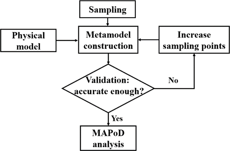
Figure 1: Flowchart of metamodel accelerated MAPoD analysis.
The flowchart starts from the sampling process. Sampling is the process to draw the values randomly according to the probability distributions of random inputs that represent uncertainty parameters, which are proposed by NDT experts or statisticians. Two sampling strategies are applied in this work: Monte Carlo sampling (MCS) and Latin Hypercube sampling (LHS). In MCS, the sampling points can be anywhere within the range of random distributions. Thus, this strategy is applied for generating the validation and prediction points. LHS divides the cumulative curves into equal intervals on the cumulative probability scale and the sampling is generated randomly in each interval. LHS avoids the sampled values from being clustered. Therefore, LHS is selected to generate the training points for the metamodel.
Subsequently, the uncertainty is propagated through the physical model for different flaw sizes. In other words, selected training points are simulated by the KD-BEM based physical model to generate the model responses. These responses are used as inputs for constructing the metamodel. To validate the metamodel, the root mean squared error (RMSE) is defined as:
| (5) |
where is the total number of validation points, and and are the prediction values and physical model responses, respectively. The normalized RMSE (NRMSE) is defined as RMSE divided by the scale of model response.
C. Metamodel
PCE is a type of stochastic metamodeling method for propagating uncertainty in the processes efficiently and can be viewed as a spectral representation of random variables in terms of polynomial basis functions which are orthogonal with respect to the probability density function of input random variables [15–17]. Based on whether it requires to reformulate or modify the existing governing equations, PCE can be categorized into intrusive and non-intrusive methods. Non-intrusive PCE considers the existing code or equations as a black box which makes it easy to implement for complex problems.
Consider a physical model represented by deterministic mapping , where is the vector of input variables, including parameters in the experiment setup and material properties. is the vector of the model response. Uncertainties in the input parameters arise during in-service inspections due to environmental conditions, human factors, and so on. In order to represent the reality of MAPoD analysis, statistical distributions of the uncertainties are introduced as inputs of the simulation model. Therefore, these uncertainties are considered in the input vector bold italicx, which is represented by a random independent vector bold italicX with prescribed probability density function. The random variables of model responses are denoted by . In PCE, the model responses bold italicY are expanded onto an orthogonal polynomial basis as [17]:
| (6) |
where is the multivariate polynomial basis, i is the index of ith polynomial term, and is the corresponding coefficient of the basis function needing to be determined. For inputs with uniform and normal distributions, the Legendre and Hermite basis are selected, respectively. In practice, a truncated form of PCE with sufficient number of terms satisfies the accuracy requirement.
The responses of a physical model are represented by a summation of PCE predictions at the same sampling points and corresponding residual:
| (7) |
where is the corresponding residual which is minimized using least squares method and P is the required number of polynomial terms:
| (8) |
where p is the required order of the PCE, n is the total number of random variables.
The LAR algorithm aims at selecting the predictors, which are the polynomial basis , that have the greatest impacts on the model response. LAR provides not only a single PC metamodel but also a collection of PC representations. The steps in the LAR algorithm are as follows [17].
Step 1: Initialize the coefficients markedasmathbolda as 0, which makes the initial residual equal to the output responses.
Step 2: Find the basis that is most correlated with the current residual, increase or decrease the coefficient of just enough such that the updated residual has as much correlation with another predictor as it does with .
Step 3: Move jointly in the direction defined by their joint least-square coefficient of the current residual until the other predictor has as much correlation with the current residual.
Step 4: Continue this procedure until the number of the predictors reaches the required numbers of samples or responses. Thus, the metamodel associated with the greatest estimate is retained.
III. NUMERICAL RESULTS
The eddy current NDT case involves a coil with finite cross section placed above a thick plate with a surface flaw as shown in Fig. 2. MAPoD analysis for different ECNDT setups and different uncertain parameters are studied. In the first setup, the coil has an inner radius 9.34 mm, outer radius 18.4 mm, length 9 mm and number of turns 408. The thick plate has thickness 12.22 mm and conductivity 30.6 MS/m. For the surface flaw, depth is 5 mm, width is 0.28 mm, and length ranges from 0.1 to 0.5 mm with the interval 0.1 mm and from 1 to 5 mm with the interval 1 mm. In the second setup, the specimen, coil parameters and defect size are changed with regard to the first one. Coil has an inner radius 6.15 mm, outer radius 12.4 mm, length 6.15 mm, and number of turns 3790. The thick plate has thickness 5 mm and conductivity 30.3 MS/m. For the surface flaw, depth is 4 mm, length is 0.5 mm, and width ranges from 0.1 to 0.5 mm with the interval 0.1 mm. Width is 0.5 mm while the length ranges from 1.5 to 3.5 mm with the interval 0.5 mm. All cases are modeled after TEAM 15 benchmark problems [22], and the accuracy of KD-BEM method for modeling has been demonstrated in [20]. Only the single position with the peak response is simulated. The PoD metrics and represent that the flaw size is with 50% and 90% probabilities of detection, respectively.
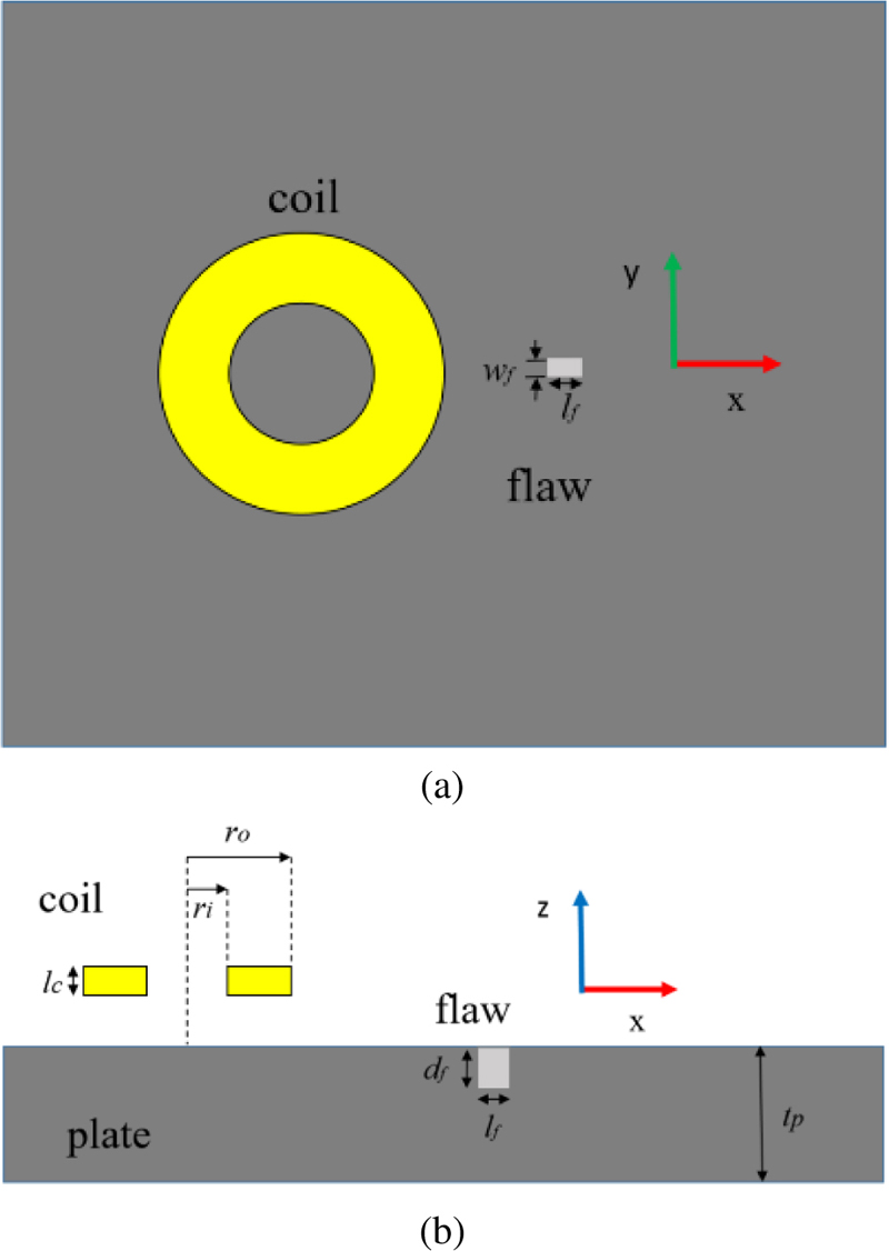
Figure 2: Sketch of ECT problem: (a) top view and (b) sectional side view.
Table 1: Distributions of the uncertain parameters
| Parameters | CASE 1 | CASE 2 | CASE 3 | CASE 4 | CASE 5 |
| Oper.Freq. (Hz) | 7000 | 7000 | 900 | 7000 | 7000 |
| x (mm) | N(13, 0.5) | U(12, 14) | N(9, 0.5) | N(14, 0.5) | U(12.5,14.5) |
| y (mm) | N(0, 0.5) | U(-1, 1) | N(0, 0.5) | U(1.5, 1.5) | U(1.5, 1.5) |
| Liftoff (mm) | N(2, 0.5) | N(2, 1) | N(2, 0.5) | U(1.83, 2.23) | N(2, 0.7) |
The relative x, y location, liftoff of the probe with respect to the flaw center, the inner and outer radius of the probe, and the tilt angle (the one between coil plane and xoy plane) are selected as the uncertain parameters with the distributions shown in Table 1. The operating frequency is 7 kHz in cases 1, 2, 4 and 5 with first setup, and 900 Hz in case 3 with second setup. In each case, 1000 MCS prediction points are generated for each flaw length/width and simulated through the KD-BEM physical model. In total (over all the flaw lengths), 5000 model responses are obtained in each case for MAPoD analysis. The model responses are the absolute values of the impedance variations which are treated in the metamodel fitting.
Convergence analysis and accuracy of proposed metamodels for surface flaw length ranges from 0.1 mm to 0.5 mm is studied in cases 1 and 2, and width ranges from 0.1 mm to 0.5 mm is studied in case 3. To test the performance of metamodels accelerated MAPoD analysis, the practical eddy current NDT cases are tested in cases 4 and 5. In cases 4 and 5, surface flaw length ranges from 1 mm to 5 mm are studied.
In case 1, to reach the predefined 1% accuracy in NRMSE and PoD metrics, the OLS-PCE method needs 500 LHS training points for each flaw length, while the LAR-PCE method needs only 150 LHS points. The computational costs are shown in Table 2. LAR-PCE only need to compute 30% physical model evaluations of OLS-PCE and the convergence of LAR-PCE is faster than OLS-PCE, which results in 72% training time savings. The NRMSE of LAR-PCE and OLS-PCE methods for flaw length ranges from 0.1 mm to 0.5 mm are shown in Fig. 3. NRMSE values are smaller than 1% for all flaw lengths. The regression line of the LAR-PCE metamodel can be found in “ vs. ” plot as shown in Fig. 4.
Table 2: Computation costs for case 1
| Model | Training Points per Flaw Length | Total TrainingTime (s) |
|---|---|---|
| OLS-PCE | 500 | 25 |
| LAR-PCE | 150 | 7 |
| Pure physicalmodel | 1000 | / |
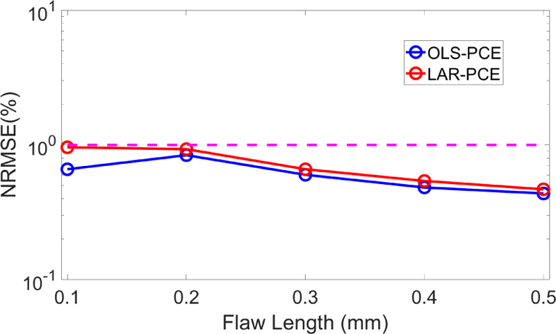
Figure 3: NRMSE of OLS-PCE with 500 LHS training points and LAR-PCE with 150 LHS training points.
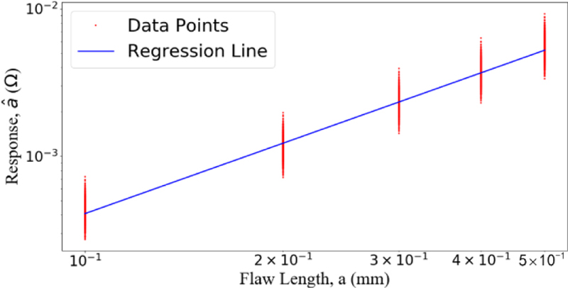
Figure 4: Case 1: “ vs. ” plot with regression line of LAR-PCE metamodel.
In Case 2, the OLS-PCE method needs 250 LHS training points, while the LAR-PCE method needs only 100 LHS training points to reach the predefined accuracy level for each flaw length. The computational costs are shown in Table 3. To reach the required accuracy level, the LAR-PCE method needs to compute 40% physical model evaluations with 63.6% training time savings over the OLS-PCE method. The regression line of the LAR-PCE metamodel can be found in “ vs. ” plot as shown in Fig. 5. Again, the LAR-PCE method accelerated physical model shows improved efficiency over the OLS-PCE method with well-maintained accuracy.
Table 3: Computation costs for case 2
| Model | Training Points per Flaw Length | Total Training Time (s) |
|---|---|---|
| OLS-PCE | 250 | 11 |
| LAR-PCE | 100 | 4 |
| Pure physical model | 1000 | / |
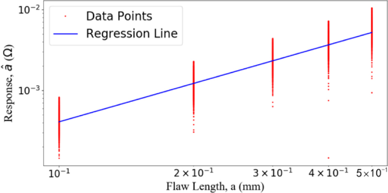
Figure 5: Case 2: “ vs. ” plot with regression line of LAR-PCE metamodel.
In case 3, flaw widths are analyzed to study the performance and accuracy of the LAR-PCE metamodel. LAR-PCE needs only 100 LHS training points while OLS-PCE needs 220 points to satisfy the accuracy level for each flaw width. Computational costs can be found in Table 4 that LAR-PCE requires 54.5% less physical model evaluations and 60% less training time than the OLS-PCE metamodel. The regression line of the LAR-PCE metamodel can be found in the “ vs. ” plot as shown in Fig. 6. Once more, the remarkable performance of the proposed LAR-PCE metamodel is demonstrated over the OLS-PCE metamodel.
Table 4: Computation costs for case 3
| Model | Training Points per Flaw Length | Total Training Time (s) |
|---|---|---|
| OLS-PCE | 220 | 15 |
| LAR-PCE | 100 | 6 |
| Pure physical model | 1000 | / |
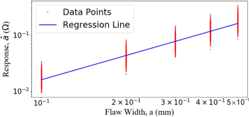
Figure 6: Case 3: “ vs. ” plot with regression line of LAR-PCE metamodel.
The LAR-PCE metamodel shows advantages over the OLS-PCE metamodel in numbers of physical model evaluation needed and training time costed with faster convergence. The performance of metamodels accelerated MAPoD analysis for practical eddy current NDT problems are considered in the following cases. Flaw lengths ranging from 1 mm to 5 mm are studied in cases 4 and 5 with different uncertain parameters. The threshold value is .
In case 4, for each flaw length, LAR-PCE and OLS-PCE need 80 and 150 training points, respectively, to reach the required accuracy level with the computational costs shown in Table 5. The OLS-PCE metamodel needs 1.88 times computational cost and 1.43 times total training time of the LAR-PCE metamodel. PoD metrics achieved by the pure physical model, LAR-PCE and OLS-PCE metamodels are shown in Table 6. The relative differences among these metrics are smaller than 1%, which satisfy the accuracy requirement. PoD curves predicted by LAR-PCE for flaw lengths are shown in Fig. 7. Both the accuracy and efficiency of the LAR-PCE metamodel over OLS-PCE are demonstrated in the practical eddy current NDT problem.
Table 5: Computation costs for case 4
| Model | Training Points per Flaw Length | Total Training Time (s) |
|---|---|---|
| OLS-PCE | 150 | 10 |
| LAR-PCE | 80 | 7 |
| Pure physical model | 1000 | / |
Table 6: PoD metrics for case 4
| Metrics | Pure Physical Model | OLS-PCE | LAR-PCE |
|---|---|---|---|
| 0.91626 | 0.91543 | 0.91564 | |
| 0.026475 | 0.027011 | 0.026402 | |
| 2.4999 | 2.4978 | 2.4984 | |
| 2.5862 | 2.5858 | 2.5844 |
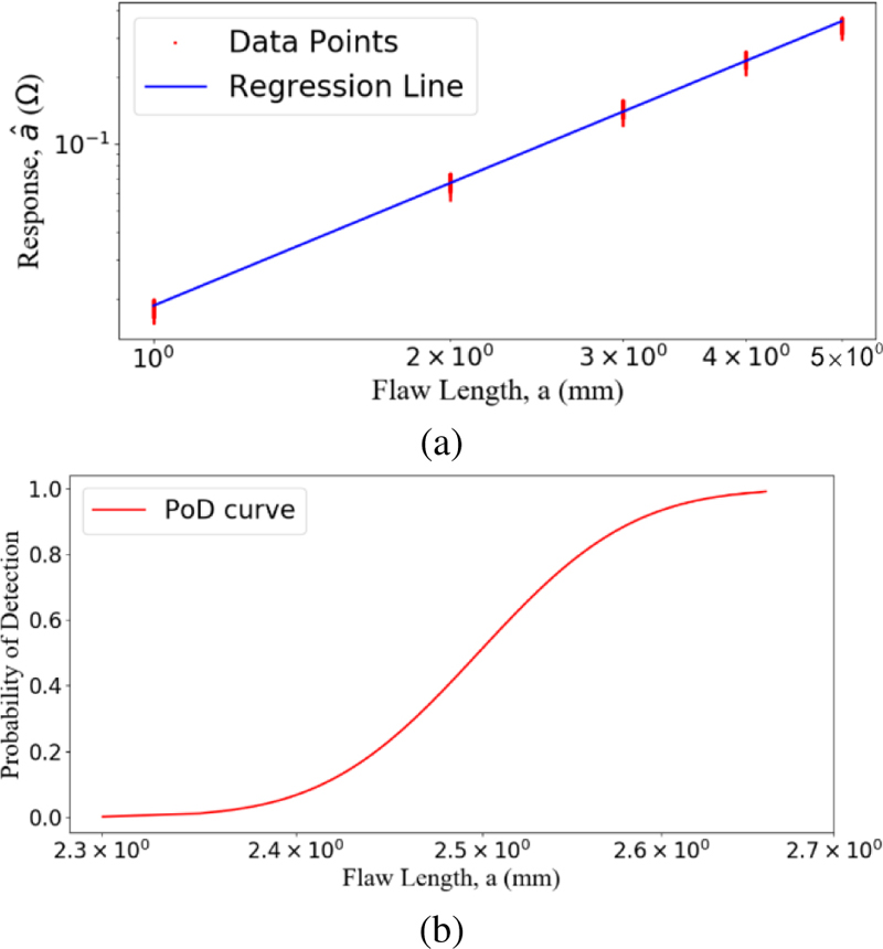
Figure 7: Case 4 (a) “ vs. ” plot with regression line of LAR-PCE metamodel and (b) PoD curves.
In case 5, PoD metrics achieved by the LAR-PCE method with 150 LHS training points, the OLS-PCE method with 500 LHS training points and the pure KD-BEM based physical model with 5000 MCS points are shown in Table 7. It can be seen that all PoD metrics predicted by the OLS-PCE and LAR-PCE agree well with those calculated by the pure physical model with the relative differences smaller than 1%. The relative differences of PoD metrics predicted by the LAR-PCE and pure physical model are 0.808%, 0.902%, 0.734% and 0.876% for , , and , respectively. The PoD curve predicted by LAR-PCE for flaw lengths is shown in Fig. 8. It can be concluded that, for case 5 to reach the required accuracy level 1% in the MAPoD analysis, the computational cost in LAR-PCE is just 30% of the OLS-PCE. This shows the advantage of applying LAR-PCE over OLS-PCE to replace the pure physical model in MAPoD analysis.
Table 7: PoD metrics for case 5
| Metrics | Pure Physical Model | OLS-PCE | LAR-PCE |
|---|---|---|---|
| 0.90845 | 0.90116 | 0.90111 | |
| 0.12531 | 0.12449 | 0.12418 | |
| 2.4805 | 2.4625 | 2.4623 | |
| 2.9126 | 2.8884 | 2.8871 |
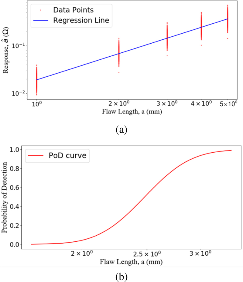
Figure 8: Case 5 (a) “ vs. ” plot with regression line of LAR-PCE metamodel and (b) PoD curves.
IV. CONCLUSION
In this paper, the LAR-PCE method is proposed to accelerate eddy current MAPoD analysis based on the KD-BEM physical model. Both the accuracy and efficiency of the LAR-PCE metamodel are demonstrated by comparing the predicted PoD metrics with the ones achieved by the OLS-PCE metamodel and the pure physical model. Through numerical tests, which include different system setups and uncertain parameters, the results show that to ensure the relative differences of PoD metrics smaller than 1.1%, the LAR-PCE metamodel needs fewer training points than the OLS-PCE model. This makes LAR-PCE more efficient than the OLS-PCE metamodel in MAPoD analysis for eddy current NDT systems. The proposed LAR-PCE metamodel should work for accelerating the MAPoD analysis regardless of achieving the physical responses from experiment or simulation only, or from both. The uncertainties considered in this study do not significantly influence the relative efficiencies of the two metamodeling techniques we compared. In other words, regardless of the uncertainties considered, the LAR-PCE based metamodel performed better than OLS-PCE, as evident from the simulation time and accuracy values. Also, it can find merits in MAPoD study in other NDT areas such as ultrasound, eddy current thermography and so on which could be the future work.
REFERENCES
[1] A. Sophian, G. Tian, D. Taylor, and J. Rudlin, “Electromagnetic and eddy current NDT: A review,” Insight, vol. 43, no. 5, pp. 302-306, 2001.
[2] J. Schijve, Fatigue of Structures and Materials. Dordrecht: Springer, 2009.
[3] M. R. Bato, A. Hor, A. Rautureau, and C. Bes, “Experimental and numerical methodology to obtain the probability of detection in eddy current NDT method,” NDT&E International, vol. 114, pp. 1-13, 2020.
[4] A. Moskovchenko, M. Švantner, V. Vavilov, and A. Chulkov, “Analyzing probability of detection as a function of defect size and depth in pulsed IR thermography,” NDT&E International, vol. 130, pp. 1-9, 2022.
[5] N. Yusa, H. Song, D. Iwata, T. Uchimoto, T. Takagi, and M. Moroi, “Probabilistic analysis of electromagnetic acoustic resonance signals for the detection of pipe wall thinning,” Nondestructive Testing and Evaluation, vol. 36, pp. 1-16, 2021.
[6] K. Tschöke, I. Mueller, V. Memmolo, M. Moix, J. Moll, Y. Lugovtsova, M. Golub, R. Sridaran, and L. Schubert, “Feasibility of model-assisted probability of detection principles for structural health monitoring systems based on guided waves for fiber-reinforced composites,” IEEE Transactions on Ultrasonics, Ferroelectrics, and Frequency Control, vol. 68, no. 10, pp. 3156-3173,2021.
[7] A. Rosell, “Efficient finite element modelling of eddy current probability of detection with transmitter–receiver sensors,” NDT&E International, vol. 75, pp. 48-56, 2015.
[8] P. Baskaran, D. J. Pasadas, A. Ribeiro, and H. Ramos, “Probability of detection modelling in eddy current NDE of flaws integrating multiple correlated variables,” NDT&E International, vol. 123, pp. 1-8, 2021.
[9] R. Miorelli, C. Reboud, T. Theodoulidis, J. Martinos, N. Poulakis, and D. Lesselier, “Coupled approach VIM–BEM for efficient modeling of ECT signal due to narrow cracks and volumetric flaws in planar layered media,” NDT&E International, vol. 62, pp. 178-183, 2014.
[10] K. Pipis, A. Skarlatos, T. Theodoulidis, and D. Lesselier, “ECT-signal calculation of cracks near fastener holes using an integral equation formalism with dedicated Green’s kernel,” IEEE Transactions on Magnetics, vol. 52. no. 4, pp. 1-8, 2015.
[11] J. Song, C. C. Lu, and W. C. Chew, “Multilevel fast multipole algorithm for electromagnetic scattering by large complex objects,” IEEE Transactions on Antennas and Propagation, vol. 45, no. 10, pp. 1488-1493, 1997.
[12] Y. Bao, Z. Liu, J. Bowler, and J. Song, “Multilevel adaptive cross approximation for efficient modeling of 3D arbitrary shaped eddy current NDE problems,” NDT&E International, vol. 104, pp. 1-9, 2019.
[13] W. Chai and D. Jiao, “An ?-matrix-based integral-equation solver of reduced complexity and controlled accuracy for solving electrodynamic problems,” IEEE Transactions on Antennas and Propagation, vol. 51, no. 10, pp. 3147-3159,2009.
[14] Y. Bao, T. Wan, Z. Liu, J. Bowler, and J. Song, “Integral equation fast solver with truncated and degenerated kernel for computing flaw signals in eddy current non-destructive testing,” NDT&E International, vol. 124, pp. 1-13, 2021.
[15] S. Bilicz, “Sparse grid surrogate models for electromagnetic problems with many parameters,” IEEE Transactions on Magnetics, vol. 52, no. 3, pp. 1-4, 2015.
[16] L. Gratiet, B. Iooss, G. Blatman, T. Browne, S. Cordeiro, and B. Goursaud, “Model assisted probability of detection curves: New statistical tools and progressive methodology,” Journal of Nondestructive Evaluation, vol. 36, no. 1, pp. 1-12,2017.
[17] G. Blatman and B. Sudret, “Adaptive sparse polynomial chaos expansion based on least angle regression,” Journal of Computational Physics, vol. 230, no. 6, pp. 2345-2367, 2011.
[18] X. Du and L. Leifsson, “Efficient uncertainty propagation for MAPOD via polynomial chaos-based Kriging,” Engineering Computations, vol. 37, no. 1, pp. 73-92, 2020.
[19] Y. Bao, “Modeling of eddy current NDT simulations by Kriging surrogate model,” Research in Nondestructive Evaluation, vol. 34, pp. 1-15, Sep. 2023.
[20] Y. Bao, Z. Liu, J. Bowler, and J. Song, “Nested kernel degeneration-based boundary element method solver for rapid computation of eddy current signals,” NDT&E International, vol. 128, pp. 1-9, 2022.
[21] S. M. Stigler, “The epic story of maximum likelihood,” Statistical Science, vol. 22, pp. 592-620, 2007.
[22] S. K. Burke, “A benchmark problem for computation of Z in eddy-current nondestructive evaluation (NDE),” Journal of Nondestructive Evaluation, vol. 7, pp. 35-41, 1988.
BIOGRAPHIES

Yang Bao was born in Nanjing, Jiangsu, China. He received the B.S. and M.S. degrees from Nanjing University of Posts and Telecommunications in 2011 and 2014, respectively, and the Ph.D. degree in Electrical Engineering from Iowa State University in 2019. Since 2019, he has been an Assistant Professor at Nanjing University of Posts and Telecommunications. His research interests focus on modeling and simulations of eddy current nondestructive evaluation.

Jiahao Qiu was born in Huai’an, Jiangsu, China. He received the B.S. degrees from Yancheng Institute of Technology in 2021. He is currently working toward the master’s degree in College of Electronic and Optical Engineering with Nanjing University of Posts and Telecommunications. His current research interests are computational electromagnetics and machine learning.

Praveen Gurrala received the B.Tech. degree from Indian Institute of Technology Madras in 2014, and the Ph.D. degree from Iowa State University in 2020, both in Electrical Engineering. He is currently a Signal Integrity Engineer at Micron Technology, Inc. His research interests include computational modeling of ultrasonic and eddy current NDE inspections, fast-multipole boundary element methods, EMI/EMC modeling and measurements, and capacitance tomography.

Jiming Song received the Ph.D. degree in Electrical Engineering from Michigan State University in 1993. From 1993 to 2000, he worked as a Postdoctoral Research Associate, a Research Scientist and Visiting Assistant Professor at the University of Illinois at Urbana-Champaign. From 1996 to 2000, he worked part-time as a Research Scientist at SAIC-DEMACO. Dr. Song was the principal author of the Fast Illinois Solver Code (FISC). He was a Principal Staff Engineer/Scientist at Semiconductor Products Sector of Motorola in Tempe, Arizona, before he joined Department of Electrical and Computer Engineering at Iowa State University as an Assistant Professor in 2002.
Dr. Song currently is a Professor at Iowa State University’s Department of Electrical and Computer Engineering. His research has dealt with modeling and simulations of electromagnetic, acoustic and elastic wave propagation, scattering, and non-destructive evaluation, electromagnetic wave propagation in metamaterials and periodic structures and applications, interconnects on lossy silicon and radio frequency components, antenna radiation and electromagnetic wave scattering using fast algorithms, and transient electromagnetic fields. He received the NSF Career Award in 2006 and is an IEEE Fellow and ACES Fellow.
ACES JOURNAL, Vol. 39, No. 5, 461–469
doi: 10.13052/2024.ACES.J.390510
© 2024 River Publishers