Study on Esophageal Tumor Detection Based on the MTV Algorithm in Electrical Impedance Imaging
Peng Ran, Wei Liu, Minchuan Li, Yingbing Lai, Zhuizhui Jiao, and Ying Zhong
1School of Bioinformatics
Chongqing University of Posts and Telecommunications, Chongqing 400065, China
LLLVVV1145@163.com, 1145059948@qq.com, s210501009@stu.cqupt.edu.cn, s220501008@stu.cqupt.edu.cn, s230501018@stu.cqupt.edu.cn
2School of Automation
Chongqing University of Posts and Telecommunications, Chongqing 400065, China
s220302003@stu.cqupt.edu.cn
Submitted On: May 16, 2024; Accepted On: September 1, 2024
ABSTRACT
This paper presents a method for detecting and locating esophageal tumors using electrical impedance tomography (EIT) based on the modified total variation (MTV) regularization algorithm, utilizing a four-layer electrode array balloon detection structure. The optimal structure of the electrode array was obtained using the uniform design (UD) method. By integrating esophageal tissue structure information, physical models containing tumors at different locations were constructed. Using the adjacent excitation mode, the study compared average voltage, voltage dynamic range, and boundary voltage changes of electrode pairs within one-quarter of a cycle to analyze esophageal tumor characteristics. By comparing the correlation coefficients, relative errors, and imaging times of three reconstruction algorithms, the MTV algorithm, which best matches the morphological characteristics of the esophagus, was selected for image reconstruction. The calculated tumor height showed an error (H) within 1 mm, indicating that EIT can provide vital information on the position, size, and electrical properties of esophageal tumors, demonstrating significant potential for clinical application in esophageal examinations.
Index Terms: Electrical impedance imaging, esophageal tumor, finite element inverse problem.
I. INTRODUCTION
Gastrointestinal tumors are a category of high-risk cancers, accounting for five of the top ten most common cancer types globally, with esophageal cancer particularly notable for its high incidence and mortality rates [1–2]. Esophageal tumors, malignant growths originating from the epithelial tissue of the esophagus, have the best treatment outcomes when detected early, hence timely detection can improve patient survival rates [3].
Traditional diagnostic methods for esophageal cancer have several limitations. For example, esophageal biopsies can cause bleeding and other complications, and CT scans are relatively expensive and involve radiation exposure. Because of the significant electrical property differences between tumor tissues and normal tissues [4], non-invasive and safe electrical impedance tomography (EIT) can reconstruct the electrical property distribution of the esophagus, obtain anatomical information, and facilitate the detection of esophageal conditions, further reflecting the positional information of pathological tissues.
EIT originated in archaeological geophysics and is characterized by functional imaging. Being non-destructive and non-invasive, it is gaining extensive application in medical diagnostics. After decades of research and innovation, EIT’s clinical utility has been confirmed in monitoring lung function [5–6] and breast cancer [7], and it has shown potential in detecting seizure zones [8], strokes [9], and cerebral edema during dehydration treatment [10]. In recent years, many research teams have started using EIT for studies on the gastrointestinal tract, primarily focusing on the stomach. Research from the Chinese Academy of Medical Sciences has shown that EIT can non-invasively detect and assess gastric motility functions [11], and scholars at home and abroad have expanded its application to studies on gastric transport, gastric emptying [12–13], and the relationship between gastric fluid pH and conductivity [14–15]. Medical diagnostics based on EIT mainly involve external monitoring devices placed outside the monitored area. Recently, intraluminal impedance tomography has also been developed. For instance, evaluating the efficacy of localized prostate cancer ablation using a multi-electrode urethral impedance probe [16], and a needle-based impedance imaging system for tissue classification [17].
However, research on esophageal wall impedance imaging is still in its early stages. In this study, utilizing the structural information and prior knowledge of the conductivity of esophageal tissues and tumors, and employing a detection balloon device with a four-layer electrode array at varying depths, we analyze esophageal tissue functions and determine the location of esophageal tumors through model design, finite element calculations, and reconstruction algorithms.
II. THEORETICAL METHOD
A. Model establishment
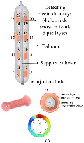
Based on the optimal structure discussed later in this paper, the model was constructed and algorithm analysis was performed using the balloon detection device shown in Fig. 1 (a). The detection balloon contains four arrays of sensing electrodes, spaced 20 mm apart, with each array consisting of six uniformly arranged electrodes. Data collection for the electric field is achieved by slowly infusing the sealed balloon, allowing the surface electrodes of the balloon to make sufficient contact with the inner wall of the esophagus.
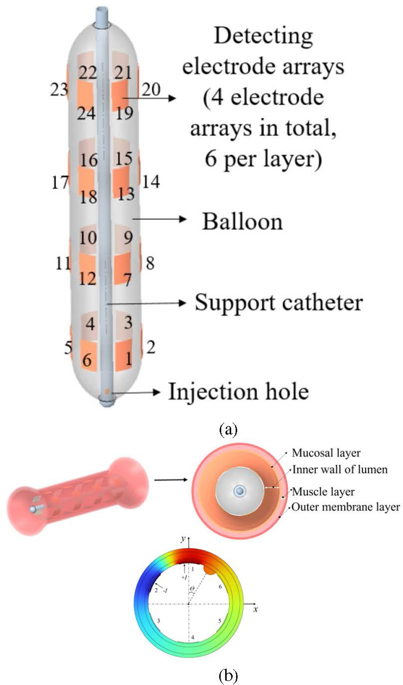
Figure 1: (a) Detection balloon and (b) esophageal model structure.
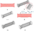
The human esophagus is approximately 25-30 cm in length, varying with individual chest lengths, has a wall thickness of 3-4 mm and a diameter of about 2 cm, and contains three narrow sections. By integrating esophageal tissue structure information, a three-dimensional EIT electric field model of a healthy esophagus and esophageal tumors was established using COMSOL to solve the forward problem. In studying the impact of the placement of a balloon within the esophagus on its morphological structure, the modeling considered two typical forms: Type 1 containing narrow sections and Type 2 without narrow sections. Healthy esophageal tissue is divided from the inside out into three layers: the mucosal layer, muscle layer, and outer layer, with respective thicknesses of 1 mm, 2 mm, and 1 mm. A two-dimensional cross-sectional structure of esophageal tissue is shown in Fig. 2 (b). The electrode-covered length of the esophagus is 10 cm, with tumors located at 5 cm (h5) and 8 cm (h8) positions in both Type 1 and Type 2, resulting in a model of the esophagus with a radius of 2, as shown in Fig. 2.

Figure 2: Three-dimensional simulation model of the esophagus: (a) Type 1 including narrow areas, (b) model 1 h5, (c) model 2 h8, (d) Type 2 excluding narrow areas, (e) model 3 h5, and (f) model 4 h8.
B. UD optimization theory
The electrode array was optimized using a uniform design (UD) method based on finite element simulation. UD was introduced by Fang and Wang [18] in 1980, utilizing number theory to uniformly distribute sampling points in space. This method enhances optimization efficiency, making it widely applicable in experiments. The general steps for multivariate optimization are as follows:
(1) Identify the variables and their search ranges, and set an appropriate number of levels for each variable.
(2) Select an appropriate UD table. Typically, a UD table is denoted as U(q), where n represents the number of experimental runs, m represents the number of variables, and each variable has q levels [19].
(3) Determine the variable combinations based on the UD table and conduct the experiments.
(4) Analyze the experimental results to identify the ”optimal” variable combination that corresponds to the maximization/minimization of the objective function.
(5) Based on the optimal variable combination, narrow down the search range for the next round of experiments. Repeat this process until the objective function stabilizes, at which point the final variable combination is obtained.
In this experiment, the standard deviation of current density is used to evaluate the uniformity of current distribution within the body. By comparing the standard deviations under different electrode array configurations, the configuration that yields the most uniform current distribution can be selected. The mathematical expression for the electrode array optimization objective function is:
| (1) |
where is the current density value at the i-th sampling point, is the mean current density, and N is the total number of sampling points.
C. Solving the forward problem
The solution to electrical impedance imaging is derived through Maxwell’s equations, which formulate a mathematical model for the electromagnetic field problem. Here, the forward problem involves knowing the conductivity distribution within a region and the boundary drive signals, and solving for the voltage distribution both inside and at the boundaries, essentially solving the boundary value problem of the electromagnetic field. The excitation current generates a specific electromagnetic field in the target area and, using electromagnetic field theory, an EIT mathematical model is constructed. The potential distribution function within the field and the conductivity distribution function satisfy the Laplace equation:
| (2) |
The boundary conditions are:
| (3) | |
| (4) |
In equations (3) and (4), represents the boundary of the field domain, represents the known boundary potential, represents the current density flowing into the field domain , and represents the outward unit normal vector of the field domain.
In the simulated esophageal model, the electrical conductivity parameters are set as follows: mucosal conductivity is 1.02 S/m, muscle conductivity is 1.16 S/m, outer layer conductivity is 0.82 S/m, and electrode conductivity is 5.9610 S/m. Tumor staging is an important means to evaluate the development of cancer, based on factors such as tumor size and depth of invasion. T1a denotes an early-stage tumor, while T2a represents an intermediate stage of cancer with a larger tumor size. To simulate different stages of tumor tissue, the esophageal lesion sizes and conductivities are set according to Table 1 in references [20–22].
Table 1: Tumor parameters of the esophagus
| Parameter | T1a | T2a |
|---|---|---|
| Radius (mm) | 2 | 3 |
| Conductivity (S/m) | 2.983.21 | 3.654.28 |
This study used 10 kHz, 5 mA alternating current for excitation. The adjacent excitation mode was employed, where current was injected between two adjacent electrode pairs, and the differential voltage was measured across other adjacent electrode pairs. This process was repeated with different electrode pairs until all pairs were used for excitation, resulting in a total of 504 boundary voltage data points used for EIT image reconstruction.
D. Image reconstruction
The inverse problem of EIT involves determining the distribution or changes in bioelectric resistivity given known voltage distributions and boundary information. A simulation was conducted using COMSOL and MATLAB, and a mesh was generated in EIDORS. The voltage data obtained from the forward simulation was used to reconstruct the esophageal EIT images using three algorithms: Laplace prior Gauss-Newton method, Tikhonov regularization, and conjugate gradient.
The Laplace prior Gauss-Newton method is performed within a Bayesian inference framework to estimate the posterior distribution of model parameters. The objective function is expressed as:
| (5) |
In this context, is the regularization factor controlling the strength of the regularization term and represents the L1 norm, which encourages sparsity in the parameters .
The motivation behind regularization methods is to address the numerical instability caused by ill-posed problems. The Tikhonov regularization method introduces a penalty term with an L2 norm to constrain the solution, and its objective function can be expressed as:
| (6) |
In equation (6), the first term is the fidelity term and the second term is the penalty term. is the regularization factor, is the estimated value obtained from prior information, and L is a specific differential operator.
Modified total variation (MTV) regularization defines the minimization objective function for three-dimensional EIT as:
| (7) |
In equation (7), represents the actual measured voltage data and represents the simulated voltage calculated based on the current conductivity distribution . and are regularization parameters that control the contribution weights of the smoothing term and the total variation term to the overall optimization problem.
This function is used with an alternating minimization method. When u is fixed in equation (8), is updated to minimize the difference with the measured voltage and the auxiliary variable. When is fixed in equation (9), u is updated to minimize the difference with and the total variation. By alternately fixing u and , the nonlinear conjugate gradient method and the split Bregman method are used to iteratively solve for and u. Convergence is checked by examining whether is less than a preset threshold or whether the maximum number of iterations has been reached:
| (8) | ||
| (9) |
The image quality is quantitatively evaluated using the correlation coefficient (CC) and relative error (RE), and the accuracy of tumor localization is assessed using the height error (H) method.
(1) Correlation coefficient
The correlation coefficient evaluates the correlation between the actual conductivity distribution and the reconstructed result, defined as:
| (10) |
(2) Image relative error
The image relative error evaluates the deviation between the reconstructed conductivity distribution and the actual conductivity distribution, assessing the deviation between the reconstructed image and the ideal image. It is defined as:
| (11) |
In this context, represents the actual distribution of electrical conductivity within the field, denotes the mean of , signifies the computed distribution of electrical conductivity, and stands for the mean of . A smaller RE and a closer CC to 1 indicate a more accurate reconstruction of the image.
(3) Height error
Establishing a coordinate system with the electrode covering the esophageal section, with the center of the bottom cross-sectional circle as the coordinate origin, let the actual height of the tumor be H and the simulated calculated height be h. Then, the height error is defined as:
| (12) |
A smaller height error, H, reflects a better reconstruction of the imaging results.
III. EXPERIMENTAL RESULTS AND ANALYSIS
A. Optimization of electrode array
Table 2 lists the five parameters to be optimized along with their respective optimization ranges. Below are the criteria and explanations for selecting these parameters:
Table 2: Electrode array optimization parameters
| Variable | Unit | Level |
|---|---|---|
| L Electrode length | mm | [5.2,14.8] |
| D Electrode width | deg | [20,32] |
| T Electrode thickness | mm | [1.2,2.4] |
| S1 Number of electrodes per layer | [3,15] | |
| S2 Number of electrode layers | [1,13] |
(1) The electrodes are attached to the surface of the balloon, with the width represented by the central angle. Furthermore, the product of the electrode unit width and the number of electrodes in a single layer must be less than 360.
(2) The product of the electrode length and the number of electrode layers must be less than the length of the target region.
(3) If the number of electrodes results in a decimal value, then it should be rounded to the nearestinteger.
Table 3 presents the UD for the first round of electrode array optimization. U(13) UD was selected, with a deviation D0.0194, indicating good uniformity that meets the design requirements of this study. The numbers in parentheses represent the sampling points of UD, and the actual optimization parameters can be calculated based on the corresponding sampling points. For example, the first sampling point combination in U(13) is (11, 6, 10, 2, 3), which corresponds to the variable combination of optimization parameters (L, D, T, S1, S2) as (13.2, 25, 2.1, 4, 3).
Table 3: UD table for the first round of electrode array parameter optimization
| No. | L | D | T | S1 | S2 |
| 1 | 13.2(11) | 25(6) | 2.1(10) | 4(2) | 3(3) |
| 2 | 9.2(6) | 27(8) | 2.4(13) | 8(6) | 10(10) |
| 3 | 8.4(5) | 32(13) | 1.4(3) | 9(7) | 2(2) |
| 4 | 6(2) | 26(7) | 1.3(2) | 13(11) | 11(11) |
| 5 | 14.8(13) | 28(9) | 1.5(4) | 12(10) | 5(5) |
| 6 | 11.6(9) | 24(5) | 1.2(1) | 7(5) | 7(7) |
| 7 | 14(12) | 21(2) | 2.3(12) | 11(9) | 1(1) |
| 8 | 6.8(3) | 22(3) | 1.9(8) | 10(8) | 12(12) |
| 9 | 7.6(4) | 31(12) | 1.6(5) | 3(1) | 9(9) |
| 10 | 5.2(1) | 29(10) | 2(9) | 6(4) | 6(6) |
| 11 | 10.8(8) | 30(11) | 1.7(6) | 5(3) | 13(13) |
| 12 | 10(7) | 20(1) | 1.8(7) | 15(13) | 4(4) |
| 13 | 12.4(10) | 23(4) | 2.2(11) | 13(12) | 8(8) |
According to the UD update method, the optimization trajectory of the electrode array is shown in Fig. 3. As can be seen from Fig. 3, after three rounds of UDs, the objective function tends to stabilize and reaches its minimum value. The optimal parameters of the electrode array are shown in Table 4.
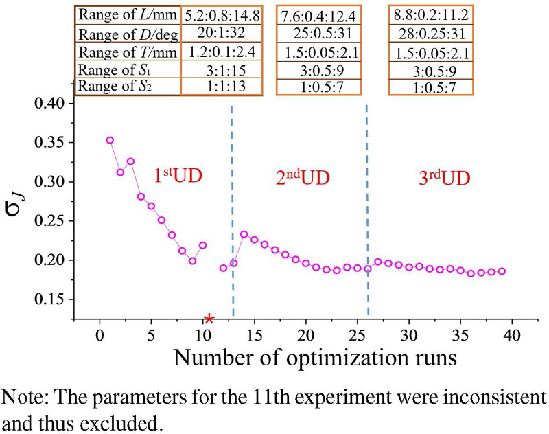
Figure 3: Trace plot of electrode array optimization.
Table 4: Optimal electrode array structural parameters
| L (mm) | D (deg) | T (mm) | S1 | S2 |
| 10 | 30 | 1.9 | 6 | 4 |
B. Positive simulation results
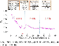
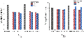
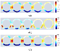
Figure 4 presents the simulation results obtained using the finite element method under uniform excitation conditions, with Fig. 4 (c) showing the two-dimensional cross-sectional electric potential distribution of esophageal tumors. There is a significant difference in the electric potential distribution between healthy esophagi and those with tumors, for the same esophageal morphology. Furthermore, when the tumor position is fixed, the electric potential distribution varies with different esophageal morphologies. Figure 5 shows the average voltage and voltage dynamic range results for six scenarios obtained by simulating the esophagus without tumors in two esophageal morphologies, and with tumors of radii 2 mm and 3 mm at positions 5 cm and 8 cm in the esophagus. The voltage dynamic range is defined as:
| (13) |
In the formula, and represent the maximum and minimum voltage, respectively.
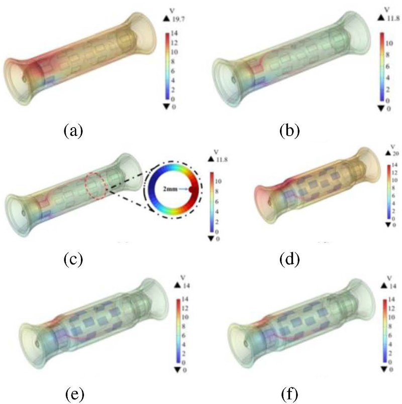
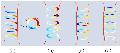
Figure 4: Simulated distribution of esophageal potential: (a) Type 1 healthy esophagus, (b) model 1, (c) model 2, (d) Type 2 healthy esophagus, (e) model 3, and (f) model 4.
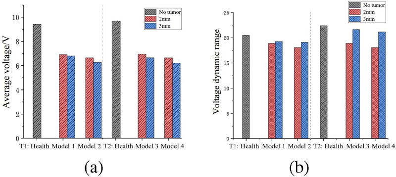
Figure 5: (a) Average voltage and (b) voltage dynamic range of different models.
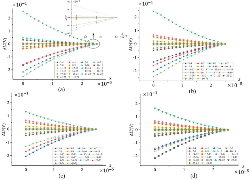
Figure 6: Relationship between changes in boundary voltage and tumor location: (a) tumor located at 30, (b) tumor located at 90, (c) tumor located at 150, and (d) tumor located at -90.
In the two types of models with tumor radii of 2 mm and 3 mm, the average voltage in the esophagus with tumors is lower than in the healthy esophagus, reflecting that the higher electrical conductivity of tumor tissue reduces the local potential. This result validates the application value of impedance imaging in distinguishing between normal and pathological esophageal tissues. Meanwhile, the smaller voltage dynamic range indicates the high quality of the model reconstruction.
To investigate the effect of tumor position at different locations on boundary voltage, Fig. 1 (b) establishes a Cartesian coordinate system for the cross-section with the tumor located at 2 cm, recording the tumor position through angles. Figure 6 shows the variation in boundary voltage during one-fourth of the excitation signal cycle when electrodes 1 and 2 are the excitation electrode pair and the tumor is located at 30, 90, 150, and -90, with the other adjacent electrodes serving as measurement electrodes. To facilitate better comparison of the data in the figure, the measurement values of electrode pair 6-7 are symmetrical about y=0. When the tumor is at 30, the adjacent electrodes are 1 and 6. It can be clearly seen from Fig. 6 (a) that the largest changes are observed in the measurement electrode pairs 5-6 and 6-7, which are adjacent to the tumor. Similarly, in Figs. 6 (b-d), it is found that the closer the electrodes are to the tumor area, the greater the changes in the relevant measurement electrode pairs. This result suggests that the trend of changes in measurement electrode pairs can be used to preliminarily locate the tumor position.
C. Reconstructed image comparison
In this study, we employed the Laplace prior Gauss-Newton method, the Tikhonov regularization algorithm, and the MTV algorithm to reconstruct EIT images of the esophageal model. The imaging results were presented as two-dimensional slices with 0.01 mm intervals. Figures 7 (a-c) illustrate the conductivity distribution of the esophagus at 4 cm, 5 cm, 6 cm, 7 cm, and 8 cm. Due to the inherent smoothness of the Tikhonov regularization algorithm, the conductivity differences between esophageal tissue and tumors were significant and had clear boundaries, resulting in a blurred boundary between the target and background regions [23]. The application of the MTV algorithm ensured the contrast of the reconstructed images, with better edge preservation, effectively mitigating the excessive smoothing issue caused by the Tikhonov algorithm. Table 2 provides a quantitative analysis of the imaging results at different layers using the correlation coefficient and relative error. Additionally, the reconstruction times for the Laplace prior Gauss-Newton method, Tikhonov regularization algorithm, and MTV algorithm were 1.163 s, 1.124 s, and 0.654 s, respectively.
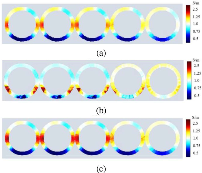
Figure 7: Reconstruction images of different layers of the esophagus: (a) GN (Laplace prior), (b) Tikhonov regularization (TK), and (c) MTV.
The results in Table 5 show that the imaging correlation coefficient of the MTV algorithm ranges from 0.797 to 0.845, and it has the smallest relative error. The imaging quality using the Laplace prior Gauss-Newton method and Tikhonov regularization algorithm is reduced by an average of 24.02% and 16.96%, respectively. Therefore, due to its superior imaging quality and real-time performance, the MTV algorithm is particularly suitable for EIT in clinical esophageal detection scenarios that require handling large-scale high-dimensional data.
Table 5: Evaluation of reconstructed images from different positions
| Algorithm | Position | CC | RE |
|---|---|---|---|
| GN | 0.706 | 0.268 | |
| TK | 4 cm | 0.814 | 0.232 |
| MTV | 0.845 | 0.196 | |
| GN | 0.723 | 0.256 | |
| TK | 5 cm | 0.784 | 0.244 |
| MTV | 0.797 | 0.213 | |
| GN | 0.687 | 0.236 | |
| TK | 6 cm | 0.765 | 0.241 |
| MTV | 0.811 | 0.217 | |
| GN | 0.715 | 0.258 | |
| TK | 7 cm | 0.782 | 0.237 |
| MTV | 0.830 | 0.193 | |
| GN | 0.692 | 0.247 | |
| TK | 8 cm | 0.812 | 0.239 |
| MTV | 0.823 | 0.201 |
Using the MTV algorithm, the conductivity was set to 3.65 S/m, 3.94 S/m, and 4.28 S/m according to the conductivity range for a tumor radius of 3 mm as shown in Table 1. Voltage data were collected for each conductivity setting, and image reconstruction was performed using the conjugate gradient algorithm. Figure 8 shows that as the conductivity increases, the color of the esophageal lesion in the reconstructed image becomes darker, which corresponds to the actual situation.
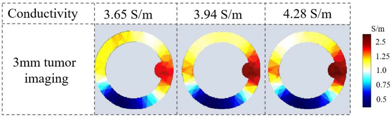
Figure 8: Tumor reconstruction image slice.
D. Positioning analysis
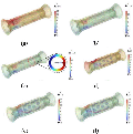
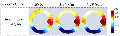
Using the MTV algorithm for EIT, the 3D reconstructions of two different esophageal shapes with 2 mm tumors located at 5 cm and 8 cm are shown in Fig. 8. The tumor locations are indicated by black arrows in Figs. 8 (b-d). Table 6 presents the tumor layer height h after imaging and the results of evaluating the 3D reconstructed esophageal tumor positions using height error H. Quantitative analysis shows that H is within 1 mm, further demonstrating that the esophageal reconstruction images obtained using this impedance imaging algorithm are closer to the original model, making tumor localization more accurate. This also proves the feasibility of using EIT for detecting esophageal tumors and its capability in localizing tumor regions.
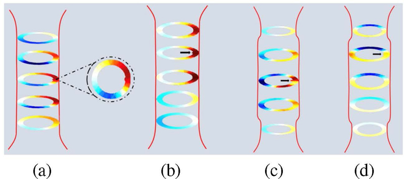
Figure 9: Results of three-dimensional reconstruction of the esophagus based on simulation data: (a) model 1, (b) model 2, (c) model 3, and (d) model 4.
Table 6: Height error of tumors at different locations
| Parameter | Model 1 | Model 2 | Model 3 | Model 4 |
|---|---|---|---|---|
| H (mm) | 50.42 | 80.90 | 40.26 | 80.86 |
| H (mm) | 0.42 | 0.90 | 0.74 | 0.68 |
IV. CONCLUSION
This study employed the UD method to optimize the electrode array and established EIT models for both healthy esophagus and esophagus with tumors at different locations. We discussed the boundary voltage changes of tumors at different positions on the same horizontal plane, noting that the measurement electrode pairs nearest to the tumor exhibited the most significant changes. This trend was used for the preliminary localization of the tumor. The Laplace prior Gauss-Newton method, the Tikhonov regularization algorithm, and the MTV algorithm were employed for image reconstruction of the esophageal model. The MTV algorithm achieved the highest imaging correlation coefficient and the smallest relative error, while requiring the least amount of time and providing the best imaging quality. MTV method was used to reconstruct the 3D structure of the esophagus, and tumor position evaluation through height error H showed that all errors were within 1 mm. This demonstrates the capability of EIT in localizing tumors.
REFERENCES
[1] R. L. Siegel, K. D. Miller, H. E. Fuchs, and A. Jemal, ”Cancer statistics, 2022,” CA: A Cancer Journal for Clinicians, vol. 72, no. 1, pp. 7-33, Jan. 2022.
[2] H. Li, J. Yu, R. Zhang, X. Li, and W. Zheng, ”Two-photon excitation fluorescence lifetime imaging microscopy: A promising diagnostic tool for digestive tract tumors,” Journal of Innovative Optical Health Sciences, vol. 12, no. 5, art. 1930009,2019.
[3] Z. Yu, X. Bai, R. Zhou, G. Ruan, M. Guo, W. Han, and H. Yang, ”Differences in the incidence and mortality of digestive cancer between Global Cancer Observatory 2020 and Global Burden of Disease 2019,” International Journal of Cancer, vol. 154, no. 4, pp. 615-625, 2024.
[4] Q. Huang, D. Lu, J. Han, H. Yu, W. Dong, K. Cai, and X. Yu, ”Comparison of dielectric properties of normal human esophagus and esophageal cancer using an open-ended coaxial probe,” Journal of Southern Medical University, vol. 41, no. 11, pp. 1741-1746, 2021.
[5] M. Xu, H. He, and Y. Long, ”Lung perfusion assessment by bedside electrical impedance tomography in critically ill patients,” Frontiers in Physiology, vol. 12, art. 748724, 2021.
[6] V. Tomicic and R. Cornejo, ”Lung monitoring with electrical impedance tomography: Technical considerations and clinical applications,” Journal of Thoracic Disease, vol. 11, no. 7, art. 3122,2019.
[7] F. Xu, M. Li, J. Li, and H. Jiang, ”Diagnostic accuracy and prognostic value of three-dimensional electrical impedance tomography imaging in patients with breast cancer,” Gland Surgery, vol. 10, no. 9, pp. 2673-2680, 2021.
[8] A. Witkowska-Wrobel, K. Aristovich, M. Faulkner, J. Avery, and D. Holder, ”Feasibility of imaging epileptic seizure onset with EIT and depth electrodes,” Neuroimage, vol. 173, pp. 311-321,2018.
[9] T. Dowrick, C. Blochet, and D. Holder, ”In vivo bioimpedance changes during haemorrhagic and ischaemic stroke in rats: Towards 3D stroke imaging using electrical impedance tomography,” Physiological Measurement, vol. 37, no. 6, pp. 765-784, 2016.
[10] B. Yang, B. Li, C. Xu, S. Hu, M. Dai, J. Xia, and F. Fu, ”Comparison of electrical impedance tomography and intracranial pressure during dehydration treatment of cerebral edema,” Neuro Image: Clinical, vol. 23, art. 101909, 2019.
[11] Z. Li and C. Ren, ”Gastric motility measurement and evaluation of functional dyspepsia by a bio-impedance method,” Physiological Measurement, vol. 29, no. 6, art. S373, 2008.
[12] M. R. Huerta-Franco, M. Vargas-Luna, J. B. Montes-Frausto, C. Flores-Hernández, and I. Morales-Mata, ”Electrical bioimpedance and other techniques for gastric emptying and motility evaluation,” World Journal of Gastrointestinal Pathophysiology, vol. 3, no. 1, pp. 10-18, 2012.
[13] R. Wicaksono, P. N. Darma, A. Inoue, H. Tsuji, and M. Takei, ”Wearable sectorial electrical impedance tomography and k-means clustering for measurement of gastric processes,” Measurement Science and Technology, vol. 33, no. 9, art. 094002, 2022.
[14] W R. Wicaksono, P. N. Darma, K. Sakai, D. Kawashima, and M. Takei, ”Imaging of gastric acidity scale by integration of pH-conversion model (pH-CM) into 3D-gastro electrical impedance tomography (3D-g-EIT),” Sensors and Actuators B: Chemical, vol. 366, art. 131923, 2022.
[15] C. S. Chaw, E. Yazaki, and D. F. Evans, ”The effect of pH change on the gastric emptying of liquids measured by electrical impedance tomography and pH-sensitive radiotelemetry capsule,” International Journal of Pharmaceutics, vol. 227, no. 1-2, pp. 167-175, 2001.
[16] J. Liu, Ö. Atmaca, and P. P. Pott, ”Needle-based electrical impedance imaging technology for Needle Navigation,” Bioengineering, vol. 10, no. 5, art. 590, 2023.
[17] Z. Cheng, D. Dall’Alba, P. Fiorini, and T. R. Savarimuthu, ”Robot-assisted electrical impedance scanning system for 2D electrical impedance tomography tissue inspection,” in Proc. 2021 43rd Annual International Conference of the IEEE Engineering in Medicine & Biology Society (EMBC), pp. 3729-3733, Nov. 2021.
[18] K. T. Fang and Y. Wang, Number-Theoretic Methods in Statistics. Boca Raton: CRC Press, 1993.
[19] K. T. Fang, D. K. Lin, P. Winker, and Y. Zhang, ”Uniform design: Theory and application,” Technometrics, vol. 42, no. 3, pp. 237-248, 2000.
[20] A. Zandi, A. Gilani, F. Abbasvandi, P. Katebi, S. R. Tafti, S. Assadi, and M. Abdolahad, ”Carbon nanotube based dielectric spectroscopy of tumor secretion; electrochemical lipidomics for cancer diagnosis,” Biosensors and Bioelectronics, vol. 142, art. 111566, 2019.
[21] D. G. Smith, S. R. Potter, B. R. Lee, H. W. Ko, W. R. Drummond, J. K. Telford, and A. W. Partin, ”In vivo measurement of tumor conductiveness with the magnetic bioimpedance method,” IEEE Transactions on Biomedical Engineering, vol. 47, no. 10, pp. 1403-1405, 2000.
[22] P. I. Wu, J. A. Sloan, S. Kuribayashi, and H. Gregersen, ”Impedance in the evaluation of the esophagus,” Annals of the New York Academy of Sciences, vol. 1481, no. 1, pp. 139-153, 2020.
[23] M. Vauhkonen, D. Vadász, P. A. Karjalainen, E. Somersalo, and J. P. Kaipio, ”Tikhonov regularization and prior information in electrical impedance tomography,” IEEE Transactions on Medical Imaging, vol. 17, no. 2, pp. 285-293, 1998.
BIOGRAPHIES
Peng Ran was born in February 1981. Ph.D., associate professor, Chongqing Innovative Young Talents Training, Chongqing smart Medical system and core technology innovation team member, Chong-qing Medical Electronics and Information Technology Engineering Research Center team member. Since 2006, he has been engaged in cutting-edge research and development of new medical equipment and detection technology.

Wei Liu was born in February 1999. Currently pursuing a master’s degree in Biomedical Engineering at the School of Bioinformatics, Chongqing University of Posts and Telecommunications. Her main research direction is the study of esophageal force electrical imaging models based on mechanical and impedance feature reconstruction.

Minchuan Li, born in September 1997, is currently a postgraduate student specializing in Biomedical Engineering at the School of Bioinformatics, Chongqing University of Posts and Telecommunications. His research is centered on advanced esophageal dynamic function detection methods, particularly focusing on piezoelectric impedance feature coupling.
Yingbing Lai was born in December 1998 and is a graduate student majoring in Biomedical Engineering at the School of Bioinformatics, Chongqing University of Posts and Telecommunications. His main research direction is the analysis of the coupling characteristics between esophageal bioelectrical impedance and mechanics.

Zhuizhui Jiao was born in February 1996. Currently a graduate student majoring in Instrument Science and Technology at the School of Automation, Chongqing University of Posts and Telecommunications. The research direction is the fluid structure coupling characteristics and dynamic functional detection methods of narrow liquid cavities.
Ying Zhong was born in October 1998. Currently studying at the School of Bioinformatics, Chongqing University of Posts and Telecommunications. Her research direction includes classification and evaluation methods for gastrointestinal diseases based on the coupling characteristics of biological impedance and biomechanics.
ACES JOURNAL, Vol. 39, No. 7, 632–641
doi: 10.13052/2024.ACES.J.390707
© 2024 River Publishers