Prediction of Antenna Performance based on Scalable Data-informed Machine Learning Methods

Yiming Chen $^{1}$ , Veysel Demir $^{2}$ , Srirama Bhupatiraju $^{3}$ , Atef Z. Elsherbeni $^{1}$ , Joselito Gavilan $^{3}$ , and Kiril Stoynov $^{3}$

¹Department of Electrical Engineering
Colorado School of Mines, Golden 80401, USA
yimingchen@mines.edu, aelsherb@mines.edu

²Department of Electrical Engineering
Northern Illinois University, Dekalb 60115, USA
vdemir@niu.edu

³Antenna Group
Nvidia, Santa Clara 95050, USA
sbhupatiraju@nvidia.com, lito.gavilan@gmail.com, kstoynov@nvidia.com

Submitted On: May 17, 2024; Accepted On: May 26, 2024

ABSTRACT

This paper proposes a scalable architecture for predicting antenna performance using various data-informed machine learning (DIML) methods. By utilizing the computation power of graphics processing units (GPUs), the architecture takes advantage of hardware (HW) acceleration from the beginning of electromagnetic (EM) full-wave simulation to the final machine learning (ML) validation. A total of 49152 full-wave simulations of a classical microwave patch antenna forms the ML dataset. The dataset contains the performance of patch antenna on six commonly used materials and two standard thicknesses in a wide frequency range from 0.1 to 20 GHz. A total of 13 base ML models are stacked and ensembled in a tabular workflow with performance as 0.970 and 0.933 F $_{1}$ scores for two classification models, as well as 0.912 and 0.819 R $_{2}$ scores for two regression models. Moreover, an image-based workflow is proposed. The image-based workflow yields the 0.823 R $_{2}$ score, indicating a near real-time prediction for all S $_{11}$ values from 0.1 to 20 GHz. The proposed architecture requires neither the fine-tuned hyperparameters in the ML-assisted optimization (MLAO) model for specified antenna design nor the pre-knowledge required in the physics-informed models. The fully automated process with data collection and the customized ML pipeline provides the architecture with robust scalability in future work where more antenna types, materials, and performance requirements can be involved. Also, it could be wrapped as a pre-trained ML model as a reference for other antenna designs.

Index Terms: Data informed, ensemble, full-wave simulation, machine learning, scalability, stacking, wide frequency range.

I. INTRODUCTION

With the unlocking of computing power, machine learning (ML) brings new prospects for non-linear and non-convex problems in higher dimensions or deeper networks. By regarding the weighting parameters as constants or a prior distribution, the Frequentist aspect [1] and Bayesian aspect [2] establish two separate systems to interpret the black-box behaviors of ML. Even though the mechanisms are different, both aspects set up similar representable matrices linking the input and output as the shared goal. Electromagnetic (EM) problems always suffer from complex input combinations, time-consuming simulations, multiple local bests, and rapid design changes. All these hindrances are exactly in line with the goal to overcome using ML. Hence, ML is undoubtedly the new perspective to explore EM problems [3, 4], and well-trained ML models could provide real-time prediction of the EM responses.

ML has been getting attention in various EM applications. For instance, at the RF system level [5–8], a customized statistical ML model combined with entropy weight theory [5] was trained by 2001 samples to predict the path loss of RF wave propagation in the very high frequency (VHF) band. ML was implemented to speed up near-field RF measurements [6] or calibrate stochastic radio propagation [7]. In [8], ML was applied to device scheduling in an over-the-air (OTA) system with lower computational loads.

From the ML point of view, as for the ML-assisted optimization (MLAO) for antenna and array designs, the traditional ML methods [9–11] demonstrated outstanding performance. For instance, the Gaussian process regression (GPR) provided the pre-knowledge guidance

to optimize array mutual coupling with low side-lobe level (SLL) [9]. The support vector regressor (SVR) was utilized to predict the magnitude and the phase of periodic units’ EM response for reflectarrays [10]. SVR also assisted in converting the polarization and reshaping the beam with an isoflux pattern [11]. Moreover, advanced deep learning (DL) and reinforcement learning (RL) were integrated into the antenna design processes [12–16]. For instance, the Bayesian neural networks (NNs) wrapping as surrogate models assisted antenna optimization with varying performance metrics [12, 13]. In [14], a computer-vision (CV) DL model combined with a traditional global optimization method, the genetic algorithm (GA), tuned the array elements for beam steering. Relying on human-like decisions with reward or penalty, RL realized automation learning in array decoupling optimization [15]. The variational autoencoders (AEs) in [16] encoded the optimum physical structure for the transmitarray design as a generativemodel.

From the antenna applications aspect, ML methods were also widely used in many antenna designs [17–20]. For example, in [17] the multiple-input multiple-output (MIMO) antenna in ultra-wideband (UWB) took advantage of the hybrid ML model to optimize the envelope correlation coefficient (ECC), diversity gain (DG), and total active reflection coefficient (TARC). This hybrid ML model was composed of SVR, GPR, and NN. Also related to the MIMO, the intelligent antenna switching, and massive MIMO in [18] achieved 18.5% higher energy efficiency over the traditional optimization methods. The RL scheme provided the optimized mapping between user elements (UE) positions and the number of active antennas during the switching in MIMO. Categorizing the information radiated from radio-frequency identification (RFID) chipless tags by utilizing ML was also a research topic. Over 99.3% accuracy was accomplished in chipless RFID measurement with five classification models [19]. Four regression models were evaluated to detect the sensing information of the 8-bit ID tag [20]. ML models also extracted high-dimensional meta-features from EM responses of on-body or implanted antennas [21–25]. For example, 1500 images in [21] were fed into convolutional neural networks (CNNs) for cancer detection.

Unlike various MLAO methods wrapped with surrogate models summarized in [26–28], data-informed machine learning (DIML) methods are explored in this paper, benefitting from a large dataset and simplicity of input/output (I/O) pairs. Data informing means all data are generated and packaged in customized formats in the first stage and then fed into the ML models in the second stage. In other words, DIMLs are regarded as “offline learning” compared to “online learning” of MLAO as a one-stage process [26]. DIML leverages generalization and scalability to include more antenna configurations with a unified format into a general model. It eliminates the consideration for the uncertain number of trials to find the local-best priori conditions in surrogate models [13, 27]. However, as a trade-off, there would be more variables from various antenna configurations to form the I/O datasets. DIML takes the fine-tuning ability of a single antenna configuration in exchange for pursuing the generalization and scalability of multiple configurations [28].

Compared with the data-informed concept, physics-informed machine learning (PIML) methods require much less data but more pre-knowledge physics. It solves the unknowns in partial differential equations (PDEs) at the high-dimensional expansions of classical EM algorithms. For example, PIMLs were applied with the Method of Moments (MoM) [29], Finite Element Method (FEM) [30], and Finite-Difference Time-Domain (FDTD) method [31, 32]. PIML mimics the behavior of numerical full-wave simulation solvers, which brings EM theoretical support to black-box prediction with the online learning surrogate. In [33], the application of PDEs transforms the classic NNs into PIML, and the proposed integral error function bypassed the pre-calculated training set with the self-learning ability. Nvidia’s “Modulus” platform provides end-to-end ML solutions for various physics problems by linking the gap between DIML and PIML methods [34].

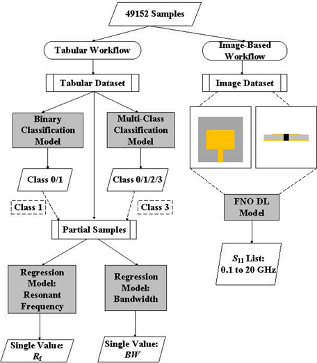
This paper presents an automated architecture utilizing the graphics processing unit (GPU) with the scalability of predicting antenna performance using DIML methods. The DIML methods are integrated with antenna design and will be necessary for our future works with PIML architecture. The general DIML architecture is presented in Fig. 1, containing two workflows utilizing a massive dataset of 49152 samples.

This paper is organized as follows. A dataset with 49152 full-wave simulations is described in Section II. The tabular workflow is demonstrated in Section III. Two classification models and two regression models based on ensemble learning are implemented to automate the predictions of antenna performance. In Section IV, the image-based workflow implements a DL NN with the Fourier Neural Operator (FNO) [35] to predict the input reflection coefficients (S $_{11}$ ) on the wide frequency range from 0.1 to 20 GHz. This neural operator is carefully designed to fit the EM frequency response with fine-tuned prediction accuracy. The conclusions and further work are presented in Section V.

Figure 1: The general architecture for the tabular and image-based workflow.

II. DATASETS

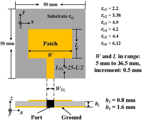
As one of the most critical parts of DIML, it is essential to construct corresponding datasets feeding into the ML models with varying prediction targets. In this paper, a classical microstrip patch antenna fed by a transmission line (TL) on various substrates is used, as shown in Fig. 2. Since the proposed architecture is for generalization purposes and not for the specific antenna fine-tuning at a pre-defined narrow band, the scalability for this architecture will be discussed in the tabular and image-based workflows in Section III and Section IV, respectively.

Figure 2: Geometry of classical patch antenna on six different substrate materials ( $ε_{r j}$ ) with two commercial thicknesses ( $h_{i}$ ), 12 combinations constitute the total dataset.

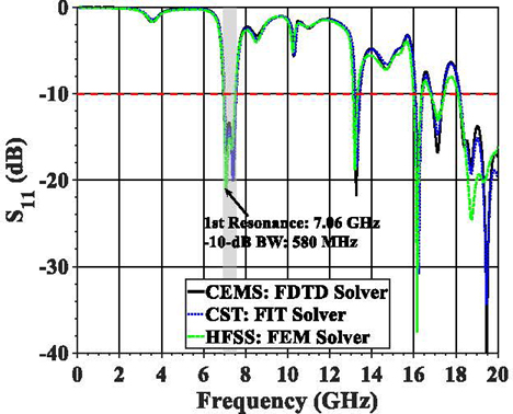
Figure 3: Simulated $S_{11}$ comparison among three full-wave simulation software with different solvers.

In Fig. 2, six materials are listed with the relative permittivity ( $ε$ $_{r}$ ) covering a relatively wide range with discrete samplings as 2.2, 3.38, 4.0, 4.2, 4.4, and 6.12. These RF materials are often commercially available as RO5880C, RO4003C, FR4 type 1, FR4 type 2, FR4 type 3, and RO4360G2 in the order mentioned. It is apparent that the $ε$ $_{r}$ sampling is denser around 4.2 because FR4 is the most commonly used material for both EM research and industry mass production by compromising material loss tangents for the low cost.

Moreover, the FR4 $ε$ $_{r}$ values 4.0, 4.2, and 4.4 are the top three values appearing in various manufacturing datasheets, considering frequency dependency, temperature dependency, material variations, and testing methods. Similarly, the thickness values 0.8 mm and 1.6 mm are two typical thicknesses on the datasheets for all six mentioned materials without extra costs of customized thickness. Six materials with two thicknesses form 12 combinations. In each combination, antenna dimensions sweep in the same way on the fixed 50 mm $\times$ 50 mm footprint size of the substrate with fully covered ground. In Fig. 2, when RO5880C is selected as the substrate (gray color) with $ε$ $_{r}$ $_{1}$ =2.2 and h $_{2}$ =1.6 mm, the 50- $Ω$ TL connects the radiating patch and the substrate edge for RF port excitation. The width W $_{TL}$ is adaptively adjusted by the substrate thickness and permittivity to achieve the 50- $Ω$ characteristic impedance. Hence, there are 12 different W $_{TL}$ values for 12 combinations of substrate. The length L $_{TL}$ is a dependent variable, making sure the TL connects the patch and the port at the substrateedge.

The radiating patch width W and length L vary from 5 mm to 36.5 mm with 0.5-mm increments, creating a 64 $\times$ 64 uniform grid-search space. Hence, there are 4096 antenna configurations in each substrate combination so, for the total dataset with 12 combinations, there are 49152 antenna configurations and, to rephrase, 49152 data samples for ML models to train and test with.

EM full-wave simulator CEMS based on FDTD method integrated with GPU acceleration [36] is used to obtain the full-wave responses for those 49152 antenna configurations at the frequency range from 0.1 to 20 GHz with 20 MHz frequency step (996 frequency points in total). Under the listed HW platform - Intel(R) Core (TM) i9-13900K; NVIDIA 4090 GPU with 24 GB memory; 128-GB DDR5 RAM at 4800 MHz - each antenna simulation takes 0.26 minutes. The time-domain (TD) solver is preset as 2000 time-steps and uniform cuboid cell sizes with increments of 0.1 mm, 0.25 mm, and 0.2 mm along x, y, and z directions, respectively. This cell size will be regarded as the image-resolution limitation in the following image-based workflow.

CEMS simulations are repeated for each of the 49152 configurations, and the input reflection coefficients are obtained as S $_{11}$ in decibel scale. For example, the result of one simulation is shown in Fig. 3. To check the consistency, simulation results from two other commercial full-wave simulation software, CST 2023 S $_{2}$ [37] and HFSS 2023 R $_{1}$ [38], are obtained to compare the simulated S $_{11}$ values as the blue dotted curve and the green dash-dotted curve in Fig. 3, respectively. As CEMS uses the TD solver (FDTD), CST also uses a TD solver but with Finite Integration Technique (FIT), while HFSS utilizes an FD solver with FEM method. The S $_{11}$ results from three simulators match with each other. Some deviations in the HFSS curve at the range higher than 18 GHz are caused by the inherent limitation of FD solvers for wide-band simulation [39].

A customized application programming interface (API) called CEMSPy is developed to automate the pipeline, from the massive generation of antenna models to the data post-processing of simulated results. Consequently, both inputs (antenna configurations) and outputs (S $_{11}$ values) are ready to feed into the black boxes to establish the I/O relationship mapping for ML models. The tabular and image-based workflows use the same dataset of 49152 samples for single value prediction in Section III and the whole S $_{11}$ curve regression in Section IV, respectively.

III. TABULAR WORKFLOW

A. Tabular datasets

For ML training based on the tabular dataset, all input features and output labels are arranged in the column-based table. The configuration information of the 49152 classical patch antenna mentioned in Fig. 2 forms 49152 rows of the tabular dataset. Five configurations, W, L, h $_{i}$ , $ε$ $_{rj}$ , and W $_{TL}$ , are regarded as five input features for the tabular workflow. This research considers S $_{11}$ values at 996 discrete points in the frequency range from 0.1 to 20 GHz as the ground-true outputs for each data sample. The output labels are the extracted observations from these simulated S $_{11}$ values. These observations could be the discrete values as the classification labels or the continuous values as the regression labels. There are two classification labels and two regression labels in the tabular workflow, which will be discussed in detail.

In a previous work related to the tabular workflow, authors have shown that more data produces higher prediction accuracy by increasing the number of samples from 256 to 4209 [40]. The authors also inspected the binary classification (BC) and single-value regression models with 20480 antenna configurations on a single substrate [41]. As a continuation of the previous work, the tabular workflow in this work extends the prediction range from 0.1 to 20 GHz to show the generalization and combines 12 different material settings to show the scalability. First, two classification models will be introduced using the 1 $^{st}$ and 2 $^{nd}$ labels in Part B of this section. Two regression models will be presented using the 3 $^{rd}$ and 4 $^{th}$ labels stored in the tabular dataset in Part C. After that, the prediction of all S $_{11}$ values at all frequencies will be discussed in Section IV.

B. Binary and multi-class classifications

As the 1 $^{st}$ output label, the BC model is trying to predict if there is a valid resonance (R $_{f}$ ) in a valid bandwidth (BW). The valid R $_{f}$ means 10% or less power reflects back to the excitation port, while the valid BW means the head and tail of -10-dB bandwidth are inside the frequency range from 0.1 to 20 GHz. The label assignments of valid R $_{f}$ and BW are packaged in CEMSPy API and can be tailored to any frequency range for specified design requirements.

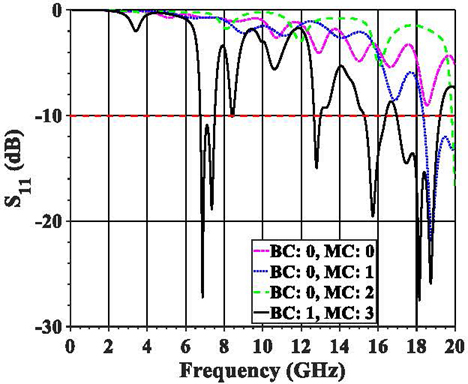
Figure 4 shows the label assignments for both the 1 $^{st}$ label of BC and 2 $^{nd}$ label of multi-class classification (MC). The same set of curves is applied to demonstrate the classification representations for both BC and 4-class MC, so there are four curves in Fig. 4.

Figure 4: Four $S_{11}$ simulation results as the classing representatives of binary classification (BC) and multi-class classification (MC).

For BC, the output at 996 frequency points having at least one valid R $_{f}$ in a valid BW can be categorized as Class 1, like the black solid curve in Fig. 4. The S $_{11}$ values in the valid band from 6.76 to 7.5 GHz are below -10 dB with two valid resonances at 6.88 and 7.36 GHz. Any other scenarios are categorized as Class 0 for BC. Under such binary strategies, 88.36% of samples in all 49152 antenna outputs are assigned in Binary Class 1 (BC: 1). The rest are assigned in Binary Class 0 (BC: 0). The definition of class assignment is demonstrated in Table 1. All 49152 samples are processed by CEMSPy and assigned the corresponding Class 0 or Class 1 for BC. The assigned binary information is stored in the tabular dataset as the 1 $^{st}$ output label. Hence, five columns as five input features (W, L, h $_{i}$ , $ε$ $_{rj}$ , and W $_{TL}$ ) and one column as the output label is poised for binary ML training and validation.

Table 1: Binary and multi-class definitions

*(R $_{f}$* , BW)**	BC	MC	Ratio of Total (%)
(0, 0)	0	0	10.38
(Valid, Invalid)	0	1	0.76
(Invalid, Invalid)	0	2	0.50
(Valid, Valid)	1	3	88.36

An automatic ML tool called “AutoGluon” builds a platform for ensemble learning on tabular datasets for both classification and regression problems [42]. Ensemble learning is a weighted strategy that combines all well-trained models as a weighted ML model to make the best predictions. Many APIs in AutoGluon provide the flexibility to customize the ensembling structure, like the selection of ML base models, the distribution of weights, etc. Associated with a customized CEMSPy script, AutoGluon is integrated into the tabular workflow to process the tabular data automatically with scalable presetting.

For BC, all 49152 samples in the total dataset are split stochastically into train/test datasets with the ratio r $_{s}$ : 80/20 under random seed 2. The same random strategy is carried through all the following work to maintain consistency and reproducibility. Those 20% samples as the test set only work for the well-trained model’s overall performance on new data after training. During the training/validation iterations, 13 base models are listed in Table 2 that are trained on 36821 samples and validated simultaneously on the remaining 2500 samples in the 39321 train dataset. Two classification metrics, F $_{1}$ score and Log loss, are used for the quantitative evaluation during the iteration of training/validation process. A total of 13 base models are updated independently towards the perfect prediction score of 1.0 and loss of 0.0 as the ideal goals. The training/validation process of 13 models will terminate when the F $_{1}$ score does not increase or Log loss no longer decreases significantly. For each sample, the F $_{1}$ score is calculated as:

F_{1} = \frac{2 T P}{2 T P + F P + F N},

(1)

where TP, often called “True Positive”, stands for the correct prediction of Class 1. Similarly, in statistical analysis, FP (False Positive) and FN (False Negative) stand for overestimation and underestimation. However, it can be noticed that TN (True Negative) is missed in the F $_{1}$ score. In other words, the scenario for the correct rejection is not counted. That is the reason why another metric Log loss is used as:

L_{\log} (y, p) = - [y \log (p) + (1 - y) \log (1 - p)],

(2)

where, p is the probability estimating label y=1 for a single sample. The averaged value F $_{1}$ score and Log loss on all test samples evaluate the general reliability of the BC model.

Table 2: Ensemble model for binary classification

Index	Model	*F $_{1}$ Score*	*LogLoss*
0	Stacked Model	0.970272	0.171912
1	KNeighborsUnif	0.968224	0.389549
2	CatBoost	0.967822	0.185379
3	KNeighborsDist	0.967149	0.386027
4	XGBoost	0.965579	0.188325
5	LightGBMLarge	0.965428	0.181846
6	ExtraTreesEntr	0.964930	0.290892
7	ExtraTreesGini	0.964856	0.286748
8	LightGBM	0.964516	0.190572
9	RandomForestEntr	0.963731	0.301912
10	RandomForestGini	0.963173	0.315406
11	NeuralNetFastAI	0.962329	0.205084
12	NeuralNetTorch	0.961868	0.185094
13	LightGBMXT	0.961072	0.197700

The final F $_{1}$ score and Log loss average on the test datasets are displayed in Table 2. The stacked model at index 0 is the weighted combination of all 13 base models from 1 to 13. As a result, when the new/unseen antenna configuration is characterized by five features, W, L, h $_{i}$ , $ε$ $_{rj}$ , and W $_{TL}$ , the stacked model can make the real-time prediction of whether there is a resonance point in a valid BW (BC: 1) or not (BC: 0). The F $_{1}$ score 0.97027 and Log loss 0.171912 indicates the ensemble model can achieve relatively reasonable prediction in the frequency range from 0.1 to 20 GHz.

For the 2 $^{nd}$ output label, the MC aims to refine the binary classes to four classes. The data categories for MC are also summarized in Table 1. For example, invalid BW means either the head or tail is out of the preset frequency range. For the blue-dotted and green-dashed curves in Fig. 4, both tails are out of 20 GHz, so these two antenna configurations are regarded as having invalid BW.

The invalid R $_{f}$ is only triggered when there is an invalid BW. According to the definition, if a valid -10-dB BW exists, at least one peak value must be inside the range. The green-dashed curve in Fig. 4 presents the antenna configuration with both invalid R $_{f}$ and BW because of the S $_{11}$ values’ monotonical decrease at the tail of the frequency range. Mirror symmetrically, if the S $_{11}$ values increase monotonically at the head range, that configuration also has invalid R $_{f}$ and BW.

An automatic pipeline has already been established for BC prediction using CEMSPy as mentioned previously. With its scalability, MC can also be implemented similarly with the slight modification of BC models. The prediction of 20% of test data achieves 0.93323 weighted F $_{1}$ and 0.2004 Log loss. However, it can also be noted in the last column of Table 1 that Class 1 (MC: 1) and Class 2 (MC: 2) have a relatively small number of samples compared to the total number of samples. As a result, it is an unbalanced MC problem in the whole frequency range, and it causes the MC model to be unbalanced and gives it an inherently high F $_{1}$ score of 0.93323. Therefore, for the unbalanced MC, an additional term called ‘balanced Acc’ is a more convincing metric to evaluate the quality of the unbalanced model:

A c c_{b a l a n c e d} = \frac{T P}{2 (T P + F N)} + \frac{T N}{2 (T N + F P)},

(3)

where TP, TN, FN, and FP follow the exact definition in (1). It gives a value of 0.55790, which is not a good score but in line with expectations due to the imbalance.

MC is not applicable for prediction in such a wide frequency range from 0.1 to 20 GHz. The application scenario would be more suitable to classify with clear objectives in narrower bands, like limiting the range to around 5.8 GHz for Wi-Fi design or around 10 GHz for space communication. In such narrow bands, the four reallocated classes will be more balanced, and the prediction will be more accurate. The CEMSPy API provides scalable functions to automate the general pipeline with the required objectives. For example, to optimize an antenna at 5.8 GHz for Wi-Fi applications, CEMSPy APIs will only simulate the models in the frequency range from 5 to 7 GHz and make the multiple-class assignment accordingly. In addition to balancing the MC, it will save significant time and computational resources to generate the I/O dataset with auto-assigned classes.

C. Single-value regressions

Unlike classification problems, single-value regression focuses on predicting a continuous value extracted from all S $_{11}$ values at 996 frequency points. In this section, the 1 $^{st}$ valid R $_{f}$ and its BW will be predicted by two regression models with similar automatic pipelines as mentioned before, but for the regression scenarios. Following the 1 $^{st}$ and 2 $^{nd}$ labels in the tabular dataset of all 49152 samples, the 3 $^{rd}$ label and 4 $^{th}$ label are assigned to the 1 $^{st}$ valid R $_{f}$ and its valid BW, respectively. Hence, the first single-value regression model could predict the 1 $^{st}$ valid R $_{f}$ for a given input set of W, L, h $_{i}$ , $ε$ $_{rj}$ , and W $_{TL}$ , and the second model for the associated BW. There is an assumption that the input antenna configuration should have a valid R $_{f}$ and valid BW. A data filter follows the class definition in Table 1. Only BC: 1 (same as MC: 3) are considered as valid samples for the two regression models. The samples in these classes are also described as “Partial Samples” in the general architecture shown in Fig. 1.

By taking 88.36% of the total 49152 samples, a truncated tabular dataset with 43431 antenna configurations is selected for two regression models. Each configuration extracts the 3 $^{rd}$ output label, R $_{f}$ in GHz, and the 4 $^{th}$ label, BW in MHz, from the corresponding S $_{11}$ values at 996 frequency points. For comparison, the 1 $^{st}$ and 2 $^{nd}$ labels are assigned as binary and multiple classes in BC and MC problems. Before the train/test splitting, 10 samples as the observers from each substrate combination (12 combinations) are dropped out randomly and stitched together as an observation dataset with 120 samples. Those samples will not be involved in any training/validation or testing process. Eventually, there are 34648, 8663, and 120 samples for training/validation, testing, and observation. The deeper reason for the observation dataset with 120 samples is that they can evenly observe the final model performance on different substrate combinations. If the model performance has a noticeable degradation in one of the 12 substrate combinations, the hyperparameters can be fine-tuned and prioritized for the respective combination separately.

Like the BC and MC pipelines, the ensemble learning method is also applied to the two single-value regression models but with deeper stacking. In the 1 $^{st}$ stacking layer, 11 base ML models produce 10 outputs as 10 new features for the 2 $^{nd}$ layer. Those 10 features are imported as the input in the 2 $^{nd}$ stacking level to predict the targeted single-value output, which is R $_{f}$ and BW, respectively. Compared with a one-layer structure with 13 flattened base models for BC and MC, each single-value regression model is weighted by 21 stacked models. One score metric called R $^{2}$ score:

R^{2} = 1 - \frac{\sum_{i = 1}^{N} (y_{i} - {\hat{y}}_{i})}{\sum_{i = 1}^{N} (y_{i} - \frac{1}{N} \sum_{i = 1}^{N} y_{i})},

(4)

and another loss metric called root-mean-squared error (RMSE):

R M S E = \sqrt{\frac{1}{N} \sum_{i = 1}^{N} {(y_{i} - {\hat{y}}_{i})}^{2}}

(5)

are enforced to increase the score and reduce the loss during each training/validation iteration. After training, (4) and (5) are applied again to evaluate the final model performance as two averaged values.

In both (4) and (5), $y_{i}$ represents the simulated value as ground true and ${\hat{y}}_{i}$ as the corresponding predicted value by regression. Theoretically, perfect regression always has a maximum score of 1.0 and a minimum loss of 0.0, like the F $_{1}$ score and Log loss for the ideal classification. The final performances for the R $_{f}$ and BW regressions are listed in Table 3. The R $^{2}$ /RMSE values for the test dataset with 8663 samples are the global representation of the well-trained models. The R $^{2}$ /RMSE ones for 120 observers are used to mimic the behavior of well-trained models when seeing new data from 12 substrate combinations evenly. The “new” here means 10 sets of (W, L, h $_{i}$ , $ε$ $_{rj}$ , and W $_{TL}$ ) from each 12 combinations that are generated randomly to observe their predicted R $_{f}$ and BW.

Table 3: Single-value regression performance

Prediction	Dataset	Samples	*R $^{2}$ Score*	*RMSE*
R $_{f}$	Test	8663	0.912440	1.171061
R $_{f}$	User	120	0.932543	1.119442
BW	Test	8663	0.818673	135.9358
BW	User	120	0.770934	162.6399

To better visualize the offset between the true value from simulation and the prediction from ML, the absolute relative error (ARE) in percentage

A R E = | \frac{y_{i} - {\hat{y}}_{i}}{y_{i}} | \times 100 %,

(6)

is used, where $y_{i}$ and ${\hat{y}}_{i}$ follow the same definition as in (4) and (5).

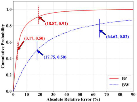
For both single-value regressions of R $_{f}$ and BW, both prediction/true offsets for 8663 samples can be calculated and stored in two ARE lists: ARE $_{R}$ $_{f}$ and ARE $_{BW}$ . The cumulative distribution function (CDF) is implemented to observe the error distribution for both regressions as shown in Fig. 5. Two markers are printed based on the cumulative probabilities of two threshold values on the solid red and the blue-dashed curves, respectively. Since the R $_{2}$ score value is a bounded value in the range [0.0, 1.0], it can be regarded as a threshold representative of the cumulative probability. The first threshold is the same as the cumulative probability 0.5 for both curves. The second threshold is the R $_{2}$ score but different for R $_{f}$ (solid red curve) and BW (blue-dashed curve). As the first vertical dashed threshold on the solid red curve, 50% of samples in total 8663 have ARE equal to or less than 3.17% for R $_{f}$ . The second threshold indicates that 91% have ARE equal to or less than 18.87%. Also, as the two thresholds on the blue-dashed curve, 50% of samples have ARE equal to or less than 17.75% for BW, and 82% have ARE equal to or less than 64.62%.

Figure 5: Cumulative distribution of absolute relative error between true and prediction for Rf and BW on 8663 test samples.

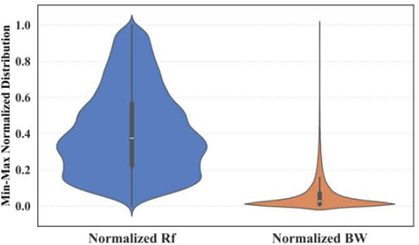
Comparing the ARE curve for BW with that for R $_{f}$ in Fig. 5, there is a dramatic degradation in BW prediction due to the resolution preset for frequency points. For the purpose of generalization, a very wide frequency range from 0.1 to 20 GHz with an incremental step of 20 MHz is utilized to show the performance on those 996 frequency points. The minimum -10 dB BW is 40 MHz because at least two values equal to or less than -10 dB could form a band. For better visualization of the value distribution, both the 3 $^{rd}$ and 4 $^{th}$ labels of all 43311 samples are normalized to the same range from 0.0 to 1.0 range based on the min-max normalization, as shown in Fig. 6. The normalized BW on the right has a much more compact distribution than that for normalized R $_{f}$ on the left. It can be expected that many antenna configurations with lower BW performance will share the same BW values (4 $^{th}$ label) under such frequency resolution.

Figure 6: Min-Max normalized distribution for both valid $R_{f}$ and valid BW on 43311 samples.

Table 4: Unique counts for R $_{f}$ and BW

Index	*R $_{f}$ (GHz)*	Counts	BW (MHz)	Counts
Top 1	8.34	118	40.0	5509
Top 2	5.80	116	60.0	4935
Top 3	7.16	111	80.0	3796
Bottom 3	19.94	1	3120.0	1
Bottom 2	3.18	1	3060.0	1
Bottom 1	3.12	1	3340.0	1

Further uniqueness analysis in Table 4 shows the extreme cases with the top-3 and bottom-3 unique counts for the 3 $^{rd}$ and 4 $^{th}$ labels of all 43311 samples. There are 839 unique R $_{f}$ values as the 3 $^{rd}$ label and 145 unique BW values as the 4 $^{th}$ label for all 43311 samples. The top-3 and bottom-3 unique counts are listed in Table 4 after sorting from largest to smallest. For example, 5509 samples of a total of 43311 have the same 40-MHz BW, which is highly concentrated compared to 118 samples with 8.34-GHz R $_{f}$ as the maximum unique counts.

From Table 4 and Fig. 6, it can be concluded that for a wide band range with such frequency resolution, the BW prediction cannot perform well due to the concentrated distribution with large identical values. As mentioned previously in the MC part, it is also a limitation of generalization, even though the BC and R $_{f}$ regression performances are reasonably good.

D. Limitation of tabular workflow

When considering generalization and scalability as the purposes, the limitation of tabular workflow is raised from two aspects. First, from the local point of view, even though the predictions are relatively good for BC and R $_{f}$ regression, the wide frequency range brings imbalance for the class definition in MC. Also, the frequency resolution limits the output uniqueness and distribution in BW regression. The first limitation can be broken by setting the narrow range for specific design requirements mentioned as the 5 to 7 GHz range for 5.8 GHz Wi-Fi antenna design in the MC part. The second limitation can be eliminated with a smaller sweeping step in the narrow range. Both concerns can be solved by utilizing the scalable CEMSPy APIs. However, it will push the model to fall into the specific local optimum and defeat the purpose of generalization. Second, from the global aspect, the tabular workflow is based on tabular datasets. Ideally, when more antenna configurations are included, users can extend the feature space along the column and the number of samples along the row to achieve scalability. However, various configurations share different parameters, and these parameters increase the complexity of constructing the tabular dataset. More configurations cause much more extensive and sparser feature space with the majority number of NaN values. Defining and unifying the variable names in tabular datasets will also be problematic. As a result, an image-based workflow is introduced in the following section. No parameter needs to be defined in the input tabular dataset; all antenna configurations will be described by the images of slice cuts from different observation planes, like magnetic resonance imaging (MRI) scanning for humantissues.

IV. IMAGE-BASED WORKFLOW

There is always a principle of DIML that post-processed data should be easy to expand at high-dimensional mapping space as the bridge connecting inputs and outputs. Inevitably, some information will be lost in the feature-extraction period from original data to post-processed data, like from the full-wave simulation model to the tabular dataset. The more information is retained from the original data, the more complicated and accurate outputs can be predicted [2]. In the tabular workflow, the original data from 49152 full-wave simulations are extracted and stored in the tabular dataset. Five input features (W, L, h $_{i}$ , $ε$ $_{rj}$ , and W $_{TL}$ ) in the five columns are applied to predict four single-value labels column by column as BC, MC, R $_{f}$ , and BW regression.

For each label in the tabular workflow, the single value is extracted from all S $_{11}$ values at 996 frequency points with presupposed conditions and assumptions. Hence, all four labels highly summarize the S $_{11}$ responses but discard lots of information in the original 996 values. It restricts the tabular workflow from achieving the purpose of generalization and scalability.

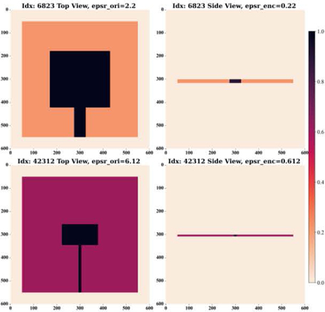
Figure 7: Encoded images of top and side views of two random samples at the index of 6823 and 42312 in total 49152 samples.

This section presents the details of the image-based workflow, showing that images carry much more input information than the tabular dataset, and the workflow will predict all the S $_{11}$ values in the whole frequency range. The same patch antenna in Fig. 2 demonstrates the image-based workflow. Two images with 600 $\times$ 600 resolutions are encoded and shown in Fig. 7. They represent two cross-sectional views of a 60 mm $\times$ 60 mm $\times$ 60 mm EM problem space. The antenna is placed at the center of the problem space based on proportional dimensions. Two cross-sectional views are selected as the observation of the patch antenna at the x-y and x-z planes in Fig. 2. All pixels in the two images are assigned the encoded values in Table 5, to represent the materials considered with EM characteristics. For instance, the pixels with values of 0.22 represent substrate material RO5880 in these pixels.

Table 5: Encoding card

Materials	Info	Encoded Value	Encoded Range
Free Space	Lossless Transmission	0.0	[0.0, 0.1]
Buffer 1	Boundary	NaN	(0.1, 0.2)
RO5880	$ε$ $_{r}$ =2.2	0.220	[0.2, 0.8]
RO4003C	$ε$ $_{r}$ =3.38	0.338	[0.2, 0.8]
FR4 Type 1	$ε$ $_{r}$ =4.0	0.400	[0.2, 0.8]
FR4 Type 2	$ε$ $_{r}$ =4.2	0.420	[0.2, 0.8]
FR4 Type 3	$ε$ $_{r}$ =4.4	0.440	[0.2, 0.8]
RO4360G	$ε$ $_{r}$ =6.12	0.612	[0.2, 0.8]
Buffer 2	Boundary	NaN	(0.8, 0.9)
Port	SMA Feed	0.9	[0.9, 1.0]
Perfect Conductor	Lossless Reflection	1.0	[0.9, 1.0]

Encoded values in the range [0.0, 1.0] are assigned to distinguish components by filling in the image pixels to represent antenna configurations with material information. Table 5 lists the encoding information for all corresponding components. There are two boundaries to split all components into three sections with enough buffering. In the middle-encoded range [0.2, 0.8], all dielectric materials are normalized in this range. Currently, the normalization factor 10 is applied on all dielectric materials, and it can be modified for scalability if the dielectric materials have relative permittivity less than 2 or larger than 8.

The two terminal values, 0.0 and 1.0, represent the free space and perfect conductor (PEC) as the lossless transmission and lossless reflection, respectively. The values can be assigned in the range [0.0, 0.1] for any lossy propagating environment. Any conducting materials with losses can be placed in the range [0.9, 1.0]. For example, the Subminiature Version A (SMA) port is assigned as 0.9. When new materials are involved, they can be designated as new values in the encoded card as new rows in Table 5. Then, new antenna configurations can pick up the values to form the images accordingly. Thus, the image-based workflow can be extended to any antenna configurations with the scalable card in Table 5.

Two encoded images for the demo configurations are displayed in Fig. 7, and they exemplify all configurations through shapes and colors. Instead of defining the variables in the tabular dataset, images carry all information in pixels, even for the different antenna types. In Fig. 7, two antenna configurations with the indices of 6823 and 42312 are selected from the total 49182 antenna samples. In the left column of Fig. 7, two top-view images embody the difference in three aspects: substrate materials, radiating patch dimensions, and width of TL. From the right column, the difference is presented in substrate thickness, width of TL, and substrate materials. Applying this encoding strategy using the integrated CEMSPy scripts, all 49152 antenna samples can be encoded and stored in a high-dimensional matrix with shape (49152, 600, 600, 2) as the ML inputs.

In the input matrix, the 1 $^{st}$ dimension shows the number of samples N $_{sam}$ , the 2 $^{nd}$ and 3 $^{rd}$ dimensions are the resolution of R $_{x}$ and R $_{y}$ , and the 4 $^{th}$ dimension is the number of the plane-cut views N $_{cp}$ . As the target of image-based workflow, all S $_{11}$ values at 996 frequency points from 0.1 to 20 GHz are predicted. Hence, the output matrix is formed in the shape (49152, 996). In the output matrix, the first dimension is the same as N $_{sam}$ for inputs, and the second dimension is the number of S $_{11}$ values at N $_{freq}$ frequency points.

So far, the I/O matrices are ready for the image-based DIML workflow. However, the I/O here is much more complicated than that for the tabular dataset. Furthermore, as the S $_{11}$ curves manifested in Figs. 3 and 4, there are correlations among adjacent points on the curves. In other words, the S $_{11}$ curve could be regarded as sequential data. Theoretically, it means for the EM response of the conjugated impedance matching at the excitation port, there should be a continuous EM response along with frequency [39]. This EM property makes the traditional ML architecture not suitable for the image-based workflow since the independent and identical distribution (i.i.d.) is often assumed in many ML models [2]. Therefore, FNO is raised as a succinct and efficient solution using an eight-layer structure with relatively faster convergence for the S $_{11}$ curve regression. It involves the EM I/O characteristics in the spectral convolutional transformations [35].

For the training/validation splitting, 152 samples are dropped out randomly only for observation purposes, as the observers mentioned in the tabular regression workflow. Then, an 80/20 splitting ratio is applied to the remaining 49000 samples. So, there are 39200 samples for training and, during the training iterations, 9800 samples are monitored to provide the performance feedback simultaneously. The model performance is optimized by evaluating the R $^{2}$ score and L $_{2}$ loss on the training and validating sets correspondingly. The R $^{2}$ score is illustrated in (4) and L $_{2}$ loss is the squared value of RMSE mentioned in (5). Second, after the training/validation process, all 152 samples are used to “observe” the well-trained models and provide the evaluation since those 152 samples are new and unseen by the well-trained model.

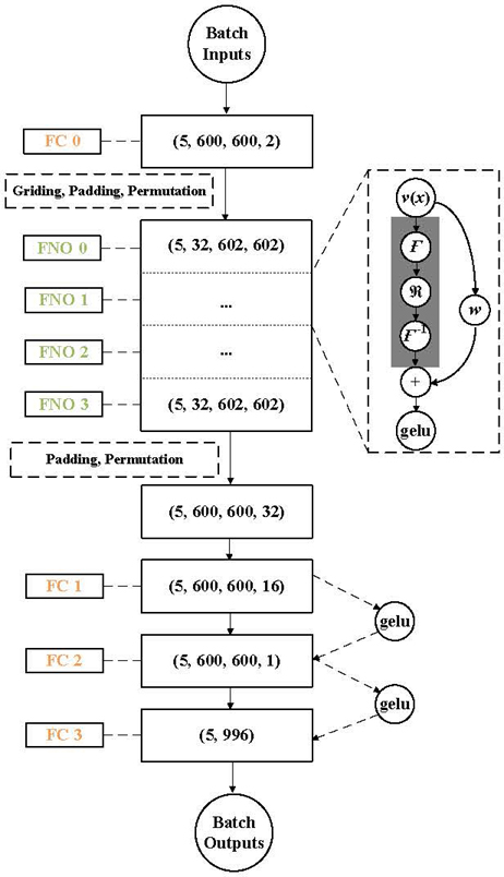
The brief NN architecture with matrix shape information is portrayed in Fig. 8, based on a single data batch with five samples. Four fully connected (FC) layers and four Fourier layers alternately construct the main skeleton of this NN used in the image-based workflow.

Figure 8: Neural network architecture with four Fourier and four fully connected layers takes five samples as a batch during optimizing the $R^{2}$ score and $L_{2}$ loss.

In the dashed zoom-in box of Fig. 8, each input v(x) processes the Fourier layers shown in the gray shadow area. The Fourier operator starts from the Fourier transform $F$ , to the linear transform $ℜ$ with a low-pass filter, then applies the inverse Fourier transform $F^{- 1}$ . During the backpropagation, the operator adjusts weights w to maximize the R $^{2}$ score and minimize L $_{2}$ loss.

By superimposing the transform and weights, the activation function Gaussian Error Linear Unit (GELU) introduces non-linearity into the model. The FNO learns the complex patterns from the images with 600 $\times$ 600 pixels. GELU provides a smooth curve, making it computationally beneficial for optimization with faster convergence during training. The same activation function is also applied to link the FC layers. Taking five samples as the batch size B $_{s}$ of a 4-D input, the variation of batch shape between NN layers is described in the intermediate flow of Fig. 8. The batch shape starts from the initial inputs with shape (B $_{s}$ , R $_{x}$ , R $_{y}$ , N $_{cp}$ ) to the final output with shape (B $_{s}$ , N $_{freq}$ ). The smoothness and nonmonotonicity of GELU bring the possibility of predicting the continuous S $_{11}$ curves at N $_{freq}$ points.

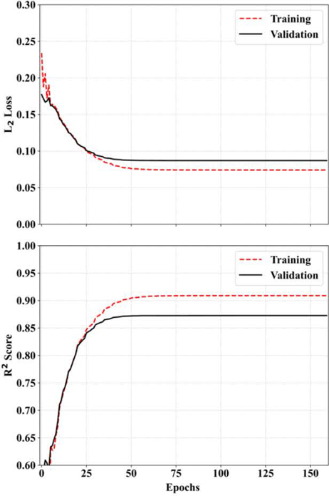
The hyperparameters in the NN architecture are fine-tuned to achieve the trade-off between the best performance of the R $^{2}$ score and L $_{2}$ loss. This workflow optimizes eight hyperparameters: learning rate L $_{r}$ , batch size B $_{s}$ , step size S $_{s}$ , gamma $Γ$ , modes N $_{\mod}$ , widths W $_{d}$ , number of FC layers N $_{FC}$ , and number of FNO layers N $_{FNO}$ . By grid searching the hyperparameter space, eight hyperparameters are selected as L $_{r}$ =0.001, B $_{s}$ =S $_{s}$ =5, $Γ$ =0.5, N $_{\mod}$ =W $_{d}$ =32, and N $_{FC}$ =N $_{FNO}$ =4. The L $_{2}$ loss and R $^{2}$ scores are achieved as 0.0742 and 0.9091 on 39200 training samples after 160 epochs and corresponding 0.0871 and 0.8728 on 9800 validation samples.

The L $_{2}$ loss and R $^{2}$ score variations with epochs are shown in Fig. 9. Both loss and score values for training and validation remain stable after 60 epochs, which indicates that the DIML model can converge and catch the prediction properly without underfitting or overfitting issues.

Figure 9: Training/validation $L_{2}$ loss and $R^{2}$ score variations with epochs.

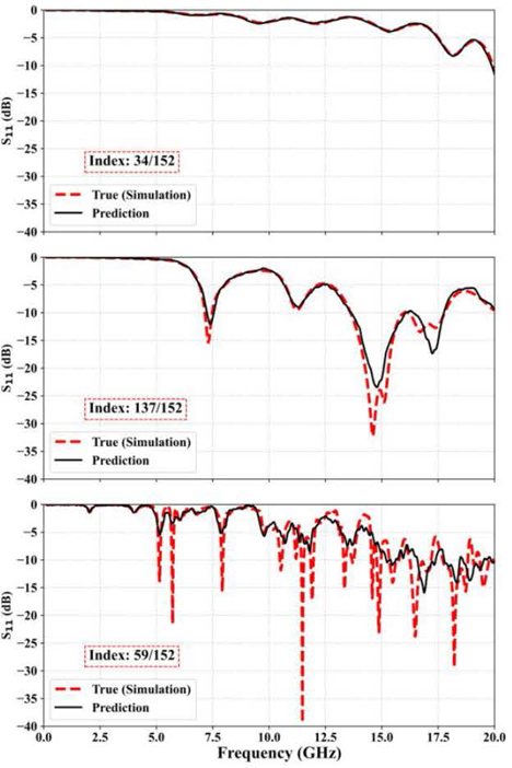
Figure 10: Representative comparison of prediction and full-wave simulation at three indexes in all 152 samples: 34, 137 and 59.

After the training/validation process with 160 epochs, 152 random samples are fed into the well-trained model to review the prediction performance on random antenna configurations. A total of 152 samples perform 0.0877 and 0.8725 for the averaged L $_{2}$ loss and R $^{2}$ score, respectively. Figure 10 compares the simulated S $_{11}$ results as ground truth and the predicted S $_{11}$ results by the FNO model on three representative antenna configurations. In each subplot of Fig. 10, the floating textbox shows the sample index in 152 total observation samples. The red-dashed curves represent the simulated S $_{11}$ results as true values. The solid black curves show the predicted S $_{11}$ when two encoded images are fed into the well-trained NNs without simulation. Moreover, for the input matrix with shape (152, 600, 600, 2), the model can make the prediction for all 152 samples in near real-time and produce an output matrix with shape (152, 996).

In the top subplot of Fig. 10, when the S $_{11}$ curve transits smoothly with less resonance along the full frequency range from 0.1 to 20 GHz, the fluctuations are relatively small. The FNO model can predict the S $_{11}$ values on all 996 frequency points very well. This case is classified as MC 0 in Table 1 with both zero R $_{f}$ and BW. In the middle subplot, this kind of S $_{11}$ response is a typical performance requirement of an alternative antenna design. The EM response has several resonances with S $_{11}$ values below -10 dB, and the impedance matching at the excitation port is conjugated harmoniously without glitches. But, in the higher frequency range, the FNO model could not predict the bands with two nearby resonances, like around 15 and 17.5 GHz. It is one topic of the authors’ following work to fine-tune the FNO model on the required narrower band. As for the bottom subplot in Fig. 10, there are more resonances and narrower BW in the whole frequency range compared to the red-dashed curves in the top and middle subplots. This causes more difficulty in prediction for the well-trained model. However, there is a tendency for the FNO model to catch all ripples on the curve. A similar observation is that the prediction at the lower frequency range is better than that at the higher frequency range.

The image-based workflow is backward compatible with all four models in the tabular workflow: BC, MC, regression for R $_{f}$ , and BW. More than that, it breaks the limitation of the tabular dataset. The plane-cut images reserve much more information from the original antenna model. The dataset is no longer bothered by pre-defined labeling and imbalanced sampling issues. The FNO model could provide a near real-time prediction close to the simulation results for a given antenna described by the encoded image. CEMSPy developers and users could customize or truncate the frequency ranges based on specific applications and then fine-tune the antenna designs.

Furthermore, the I/O data formats allow generalization and scalability when more antenna configurations are involved. As the input matrix follows the shape (49152, 600, 600, 2), sample numbers at the 1 $^{st}$ dimension will be increased if there are more configurations. More complicated configurations add more plane-cut views at the 4 $^{th}$ dimension. Those views describe the antenna structure from different observation directions. The 4 $^{th}$ dimension will always consider the maximum number of views compatible with different antennas. If some antennas don’t need specific views, those images will be filled with NaN values to keep the uniform number of views at the 4 $^{th}$ dimension. A total of 600 $\times$ 600 pixels at the 2 $^{nd}$ and 3 $^{rd}$ dimensions could accommodate the 0.1-mm dimension changes in the design. When considering the fabrication tolerance, this resolution is adequate in antenna design, and users can refine it. This 0.1-mm dimension is also the limitation of the CEMS cell size setting. In the current simulations, the minimum cell size is 0.1 mm along the x direction, and the other two cell sizes are 0.25 mm and 0.2 mm along the y and z directions, respectively. The image resolution and the CEMS cell size both ensure that the simulation results can be relied on as the true values in ML regression.

In the view of input encoded images, colors will hold all material information in the images with 600 $\times$ 600 resolution. Users can pick the color from the encoded card in Table 5 and then fill all pixels using the CEMSPy API for all plan-cut views. In the case there is no required material in the card, users can define the encoded values derived from the corresponding encoded ranges with solid boundaries. From another view of the output shape (49152, 996), the 1 $^{st}$ dimension keeps the one-on-one mapping with the 1 $^{st}$ dimension of inputs. The 2 $^{nd}$ dimension reserves a list of predicted values for each sample. In this general workflow, it is an S $_{11}$ list with 996 frequency points. Similarly, it can be the list like voltage standing wave ratio (VSWR), maximum gain (G), minimum axial ratio (AR), and so on. By modifying the final FC layer structure in the FNO model presented in Fig. 8, the pipeline could also predict the 2D matrix, like the whole spherical radiation pattern at defined frequency points.

However, there are also limitations to this image-based workflow. First, as for the input, since it only demonstrates the generalization and scalability purpose, only a classic patch antenna is utilized as the proof of concept. The authors’ following work will generate a more diverse dataset in which there are more antenna configurations as input. Second, only S $_{11}$ values are predicted as output in the current image-based workflow, and no other antenna performance is involved. It will be the extended work of this pipeline to consider more radiation parameters as output. For any developers or users applying the tabular or image-based workflow, except for customizing the antenna configuration and performance requirements, all parts will remain the same as the proposed workflow by applying the automatic pipeline with integrated CEMSPy APIs. The scalable pipeline will handle all work from simulation, data post-processing, and ML training to validation. Unlike the MLAO models, both tabular and image-based workflows are freed from the cost function customized by the trial-and-error approach, and neither need to calibrate the parameters with ML assistance during the iteration. CEMSPy packages all work inside the DIML black box in the training/validation process. With the well-trained model, users could get near-real-time predictions based on tabular or image inputs.

V. CONCLUSION

This paper proposes an automated architecture to predict the antenna performance S $_{11}$ values using the DIML methods in different data-format levels. The tabular and image-based workflows take the same 49152 samples with 12 different material combinations but utilize different dataset formats. Both exhibit the properties of scalability and generalization from various points of view. In the tabular workflow, the binary and multi-class classifications achieved 0.970 and 0.933 F $_{1}$ scores on the test dataset with 9831 samples. The single-value regression models for R $_{f}$ and BW accomplished 0.912 and 0.819 R $_{2}$ scores on 8663 test samples. In the image-based workflow, the 9800 validation samples reached a 0.873 R $_{2}$ score for prediction after hyperparameter optimization in the FNO DL model. The scalable workflows and the easy-to-append dataset format give the architecture great potential to accommodate other antenna types and more diverse performance needs. It can be regarded as a pre-trained model for other projects. This DIML is also a necessary part of the future PIML work, with much fewer samples required.

ACKNOWLEDGMENT

The author would like to thank Dr. Zhiwei Fang for providing valuable technical support related to deep learning architecture applied in the image-basedworkflow.

REFERENCES

[1] C. M. Bishop and M. N. Nasser, Pattern Recognition and Machine Learning. New York: Springer, 2006.

[2] K. P. Murphy, Machine Learning: A Probabilistic Perspective. Cambridge, MA: MIT Press, 2012.

[3] M. Martínez-Ramón, A. Gupta, J. L. Rojo-Álvarez, and G. C. Christos, Machine Learning Applications in Electromagnetics and Antenna Array Processing. London: Artech House, 2021.

[4] M. Li and S. Marco, Applications of Deep Learning in Electromagnetics: Teaching Maxwell’s Equations to Machines. London: IET, 2023.

[5] J. Wang, Y. Hao, and Y. Cheng, “A comprehensive prediction model for VHF radio wave propagation by integrating entropy weight theory and machine learning methods,” IEEE Transactions on Antennas and Propagation, vol. 71, no. 7, pp. 6249-6254, Apr. 2023.

[6] R. R. Alavi, R. Mirzavand, J. Doucette, and P. Mousavi, “An adaptive data acquisition and clustering technique to enhance the speed of spherical near-field antenna measurements,” IEEE Antennas and Wireless Propagation Letters, vol. 18, no. 11, pp. 2325-2329, Aug. 2019.

[7] R. Adeogun, “Calibration of stochastic radio propagation models using machine learning,” IEEE Antennas and Wireless Propagation Letters, vol. 18, no. 12, pp. 2538-2542, Sep. 2019.

[8] A. Bereyhi, A. Vagollari, S. Asaad, R. R. Müller, W. Gerstacker, and H. V. Poor, “Device scheduling in over-the-air federated learning via matching pursuit,” IEEE Transactions on Signal Processing, vol. 71, pp. 2188-2203, June 2023.

[9] Q. Wu, W. Chen, C. Yu, H. Wang, and W. Hong, “Knowledge-guided active-base-element modeling in machine-learning-assisted antenna-array design,” IEEE Transactions on Antennas and Propagation, vol. 71, no. 2, pp. 1578-1589, Feb. 2023.

[10] M. Salucci, L. Tenuti, G. Oliveri, and A. Massa, “Efficient prediction of the EM response of reflectarray antenna elements by an advanced statistical learning method,” IEEE Transactions on Antennas and Propagation, vol. 66, no. 8, pp. 3995-4007, May 2018.

[11] D. R. Prado, P. Naseri, J. A. López-Fernández, S. V. Hum, and M. Arrebola, “Support vector regression-enabled optimization strategy of dual circularly-polarized shaped-beam reflectarray with improved cross-polarization performance,” IEEE Transactions on Antennas and Propagation, vol. 71, no. 1, pp. 497-507, Oct. 2022.

[12] B. Liu, M. O. Akinsolu, C. Song, Q. Hua, P. Excell, Q. Xu, Y, Huang, and M. A. Imran, “An efficient method for complex antenna design based on a self adaptive surrogate model-assisted optimization technique,” IEEE Transactions on Antennas and Propagation, vol. 69, no. 4, pp. 2302-2315, Jan. 2021.

[13] Y. Liu, B. Liu, M. Ur-Rehman, M. A. Imran, M. O. Akinsolu, P. Excell, and Q. Hua, “An efficient method for antenna design based on a self-adaptive Bayesian neural network-assisted global optimization technique,” IEEE Transactions on Antennas and Propagation, vol. 70, no. 12, pp. 11375-11388, Oct. 2022.

[14] V. Loscrí, C. Rizza, A. Benslimane, A. M. Vegni, E. Innocenti, and R. Giuliano, “BEST-RIM: A mm wave beam steering approach based on computer vision-enhanced reconfigurable intelligent metasurfaces,” IEEE Transactions on Vehicular Technology, vol. 72, no. 6, pp. 7613-7626, Feb.2023.

[15] Z. Wei, Z. Zhou, P. Wang, J. Ren, Y. Yin, G. F. Pedersen, and M. Shen, “Fully automated design method based on reinforcement learning and surrogate modeling for antenna array decoupling,” IEEE Transactions on Antennas and Propagation, vol. 71, no. 1, pp. 660-671, Jan. 2023.

[16] P. Naseri and S. V. Hum, “A generative machine learning-based approach for inverse design of multilayer metasurfaces,” IEEE Transactions on Antennas and Propagation, vol. 69, no. 9, pp. 5725-5739, Sep. 2021.

[17] D. Sarkar, T. Khan, and A. A. Kishk, “Machine learning assisted hybrid electromagnetic modeling framework and its applications to UWB MIMO antennas,” IEEE Access, vol. 11, pp. 19645-19656, Feb. 2023.

[18] M. Hoffmann and K. Pawel, “Reinforcement learning for energy-efficient 5G massive MIMO: Intelligent antenna switching,” IEEE Access, vol. 9, pp. 30329-130339, Sep. 2021.

[19] F. Villa-Gonzalez, J. J. F. Sokoudjou, O. Pedrosa, D. Valderas, and I. Ochoa, “Analysis of machine learning algorithms for USRP-based smart chipless RFID readers,” 2023 17th European Conference on Antennas and Propagation (EuCAP), Florence, Italy, pp. 1-5, May 2023.

[20] N. Rather, R. B. Simorangkir, J. Buckley, B. O’Flynn, and S. Tedesco, “Evaluation of machine learning models for a chipless RFID sensor tag,” 2023 17th European Conference on Antennas and Propagation (EuCAP), Florence, Italy, pp. 1-5, May 2023.

[21] S. Costanzo, A. Flores, and G. Buonanno. “Fast and accurate CNN-based machine learning approach for microwave medical imaging in cancer detection,” IEEE Access, vol. 11, pp. 2169-3536, June 2023.

[22] Y. Kim and Y. Li, “Human activity classification with transmission and reflection coefficients of on-body antennas through deep convolutional neural networks,” IEEE Transactions on Antennas and Propagation, vol. 65, no. 5, pp. 2764-2768, Mar. 2017.

[23] S. K. Singh and A. N. Yadav, “Machine learning approach in optimal localization of tumor using a novel SIW-based antenna for improvement of ablation zone in hepatocellular carcinoma,” IEEE Access, vol. 11, pp. 26964-26978, Mar. 2023.

[24] E. N. Paulson, H. Park, J. Lee, and S. Kim, “Machine learning-based joint vital signs and occupancy detection with IR-UWB sensor,” IEEE Sensors Journal, vol. 23, no. 7, pp. 7475-7482, Feb. 2023.

[25] F. Zardi, M. Salucci, L. Poli, and A. Massa, “SbD-driven microwave imaging for biomedical diagnosis,” 2023 17th European Conference on Antennas and Propagation (EuCAP), Florence, Italy, pp. 1-4, May 2023.

[26] Q. Wu, Y. Cao, H. Wang, and W. Hong, “Machine-learning-assisted optimization and its application to antenna designs: Opportunities and challenges,” China Communications, vol. 17, no. 4, pp. 152-164, Apr. 2020.

[27] H. M. El Misilmani, T. Naous, and S. K. Al Khatib, “A review on the design and optimization of antennas using machine learning algorithms and techniques,” International Journal of RF and Microwave Computer-Aided Engineering, vol. 30, no. 10, pp. e22356, Oct. 2020.

[28] H. M. El Misilmani and T. Naous, “Machine learning in antenna design: An overview on machine learning concept and algorithms,” 2019 International Conference on High Performance Computing & Simulation (HPCS), Dublin, Ireland, pp. 600-607, Sep. 2019.

[29] H. M. Yao, L. J. Jiang, and Y. W. Qin, “Machine Learning based Method of Moments (ML-MoM),” in 2017 IEEE International Symposium on Antennas and Propagation & USNC/URSI National Radio Science Meeting, San Diego, CA, pp. 973-974, July 2017.

[30] T. Özdemir, D. N. Aloi, K. Bi, and R. J. Burkholder, “Numerical mesh truncation boundary conditions optimized via machine learning,” in 2019 International Applied Computational Electromagnetics Society Symposium (ACES), Miami, FL, pp. 1-2, Apr. 2019.

[31] H. M. Yao and L. J. Jiang, “Machine-learning-based PML for the FDTD method,” IEEE Antennas and Wireless Propagation Letters, vol. 18, no. 1, pp. 192-196, Jan. 2019.

[32] H. M. Yao and L. J. Jiang, “Machine learning based neural network solving methods for the FDTD method,” in 2018 IEEE International Symposium on Antennas and Propagation & USNC/URSI National Radio Science Meeting, Boston, MA, pp. 2321-2322, July 2018.

[33] S. Barmada, P. D. Barba, A. Formisano, M. E. Mognaschi, and M. Tucci, “Physics-informed neural networks for the resolution of analysis problems in electromagnetics,” ACES Journal, vol. 38, no. 11, pp. 841-848, Nov. 2023.

[34] https://docs.nvidia.com/deeplearning/modulus/modulus-v2209/index.html.

[35] Z. Li, N. Kovachki, K. Azizzadenesheli, B. Liu, K. Bhattacharya, A. Stuart, and A. Anandkumar, “Fourier neural operator for parametric partial differential equations,” [Online]. Available: arXiv:2010.08895, Oct. 2020.

[36] V. Demir and A. Z. Elsherbeni, “Computational Electromagnetics Simulator (CEMS),” Available: veysdemir@gmail.com, version 5, Oct. 2023.

[37] Simulia CST Microwave Studio, ver. 2023 S $_{2}$ , Dassault Systems Simulia Corp, Framingham, MA, 2023.

[38] Ansys High Frequency Structure Simulation (HFSS), ver. 2023 R $_{1}$ , Ansys Inc, Canonsburg, PA, 2023.

[39] A. Z. Elsherbeni and V. Demir, The Finite-Difference Time Domain Method for Electromagnetics with MATLAB Simulations, 2nd ed. Raleigh: SciTech Publishing, pp. 169-184, Nov. 2015.

[40] Y. Chen, A. Z. Elsherbeni, and V. Demir, “Machine learning for microstrip patch antenna design: Observations and recommendations,” in 2022 United States National Committee of URSI National Radio Science Meeting (USNC-URSI NRSM), Boulder, CO, pp. 256-257, Jan. 2022.

[41] Y. Chen, A. Z. Elsherbeni, and V. Demir, “Machine learning design of printed patch antenna,” in 2022 IEEE International Symposium on Antennas and Propagation and USNC-URSI Radio Science Meeting (AP-S/URSI), Denver, CO, pp. 201-202, July 2022.

[42] https://auto.gluon.ai/stable/index.html.

BIOGRAPHIES

Yiming Chen received the M.S. degree in Electrical Engineering from the China University of Mining and Technology, Xuzhou, China, in 2019. Currently, he is a Ph.D. candidate from the ARC group at the Department of Electrical Engineering, Colorado School of Mines, Colorado, USA. His interests are in antenna design with machine learning, metasurface array optimization, on-body antenna, and RFID.

Veysel Demir is an Associate Professor at the Department of Electrical Engineering at Northern Illinois University, USA. He received his Bachelor of Science degree in Electrical Engineering from Middle East Technical University, Ankara, Turkey, in 1997. He studied at Syracuse University, New York, where he received both a Master of Science and Doctor of Philosophy degrees in Electrical Engineering in 2002 and 2004, respectively. During his graduate studies, he worked as a Research Assistant for Sonnet Software, Inc., Liverpool, New York. He worked as a visiting Research Scholar in the Department of Electrical Engineering at the University of Mississippi from 2004 to 2007. He joined Northern Illinois University in August 2007 and served as an Assistant Professor until August 2014. He has been serving as an Associate Professor since then.

Srirama Bhupatiraju received his master’s degree in telecommunication engineering from the University of Texas, Dallas, USA, in 2012. He is a Senior Antenna Engineer with the Wireless and Radio Group at Nvidia, Santa Clara, USA. He has 10+ years of experience in the consumer electronics industry and his areas of interests are high performance computing, Desense, EMI, Antenna, and RF system design.

Atef Z. Elsherbeni received an honor B.Sc. degree in Electronics and Communications, an honor B.Sc. degree in Applied Physics, and a M.Eng. degree in Electrical Engineering, all from Cairo University, Cairo, Egypt, in 1976, 1979, and 1982, respectively, and a Ph.D. degree in Electrical Engineering from Manitoba University, Winnipeg, Manitoba, Canada, in 1987. He started his engineering career as a part time Software and System Design Engineer from March 1980 to December 1982 at the Automated Data System Center, Cairo, Egypt. From January to August 1987, he was a Post-Doctoral Fellow at Manitoba University. Dr. Elsherbeni joined the faculty at the University of Mississippi in August 1987 as an Assistant Professor of Electrical Engineering. He advanced to the rank of Associate Professor in July 1991, and to the rank of Professor in July 1997. He was the Associate Dean of the College of Engineering for Research and Graduate Programs from July 2009 to July 2013 at the University of Mississippi. He then joined the Electrical Engineering and Computer Science (EECS) Department at Colorado School of Mines in August 2013 as the Dobelman Distinguished Chair Professor. He was appointed the Interim Department Head for EECS from 2015 to 2016 and from 2016 to 2018 he was the Electrical Engineering Department Head. He spent a sabbatical term in 1996 at the Electrical Engineering Department, University of California at Los Angeles (UCLA) and was a visiting Professor at Magdeburg University during the summer of 2005 and at Tampere University of Technology in Finland during the summer of 2007. In 2009 he was selected as Finland Distinguished Professor by the Academy of Finland and TEKES. Dr. Elsherbeni is an IEEE Life Fellow and ACES Fellow. He is the Editor-in-Chief for ACES Journal, and a past Associate Editor to the Radio Science Journal. He was the Chair of the Engineering and Physics Division of the Mississippi Academy of Science, the Chair of the Educational Activity Committee for IEEE Region 3 Section, and the general Chair for the 2014 APS-URSI Symposium and the President of ACES Society from 2013 to 2015. Dr. Elsherbeni is selected as Distinguished Lecturer for IEEE Antennas and Propagation Society for 2020-2023. He is the recent recipient of the 2023 IEEE APS Harington-Mittra Award for his contribution to computational electromagnetics with hardware acceleration.

Joselito Gavilan holds a B.S. degree in Electrical Engineering and a master’s in engineering degree with a focus on Electromagnetics and Wireless Communication, both earned from the University of Illinois at Chicago in ’98 and ’04 respectively. Joselito has over 20 years of product design experience, ranging from base station antenna products to mobile phones, tablets, laptops, gaming devices, and high-performance edge computers. His interest is product integration and simulation. He enjoys the challenges of tight integration and learning the constraints of cross-functional disciplines to make the right tradeoffs. Currently, he is at NVIDIA, leading efforts to reimagine computational simulations given the accessibility of high-performance supercomputers and AI technologies.

Kiril Stoynov received the M.S. degree in Electrical Engineering with concentration in Computational Electromagnetics from the University of Akron in 2008. Currently he is an EPM in the Systems Products Team at Nvidia working on Industrial and Embedded Products. Kiril has interests in antenna design, simulations, HPC, AI and simulations on a large scale.