Deep Learning-Based Hybrid Multivariate Improved ResNet and U-Net Scheme for Satellite Image Classification to Detect Targeted Region
P. Pabitha Muthu, S. Siva Ranjani, and M. Manikandakumar
1Sethu Institute of Technology
Kariapatti, Virudhunagar District-626115, Tamil Nadu, India
pabithapraveen@gmail.com, Sivaranjani222@gmail.com
2Department of AIML and Data Science
Christ University, Kengeri Campus, Karnataka-560074, India
manikandakumar.m@christuniversity.in
Submitted On: June 13, 2024; Accepted On: July 25, 2025
ABSTRACT
In the field of remote sensing, the process of segmentation and classification of satellite images is a challenging task attributable to different types of target detection. There are problems in recognizing a target and clutter region. Then, there is a necessity to consider these problems regarding the classification of satellite image using an effectual approach. In this approach, a deep learning dependent automated segmentation, detection, and classification of satellite images is carried with artificial intelligence methods. Initially, the input image is preprocessed, segmented using Edge-ROI and YOLO v3 based segmentation in which the parameter is tuned by means of multi-heuristic tuna swarm optimization (MH-TSO) approach and is classified using hybrid multivariate improved residual network (ResNet) and U-Net classifier approach. The stage of Edge-ROI segmentation and YOLO v3 based segmentation is employed to extract regions. The preprocessing is carried using median average filtering along with adaptive histogram equalization. A scheme of deep learning-based multivariate improved residual neural network for classification of satellite images is proposed effectively. The proposed technique performance is estimated for three kinds of dataset, namely Salinas, Pavia University, and Indian Pines satellite image datasets, and the results obtained are shown, which proves the efficiency of the suggested mechanism.
Index Terms: Hybrid multivariate improved residual neural network and U-Net, multi-heuristic tuna swarm optimization, remote sensing, satellite image, YOLO v3 segmentation.
I. INTRODUCTION
At present, scholars have focused on image classification which is thus regraded as a pivotal technology for the recognition of pattern and a computer vision scheme. Usually, the satellite images are in a digital form [1]. The technique of image processing could be employed for the retrieval of precise set of data from the stored images [2][3]. Therefore, this technique will be obliging in improving the visual perception and to modify or repair an image which depends on blurring of image, image deformation, or image deterioration [4]. Few methods are still available to analyze the image which relies on some specified issue requirements [5-7]. Image segmentation and classification algorithms are utilized in various regions of image in a thematic group. The kinds of image segmentation are categorized as four types from varied range of angles like feature space clustering, region-based, model-driven, and threshold-based [8,9]. Presently, the feature space clustering approach is regarded as the most significant and popular method for image segmentation due to its easy calculation, simple principle, and good segmentation. Furthermore, the images are normally segmented using a single clustering technique, and it is probable to get stuck in a local optimum since the boundaries are blurred and this displays unclear boundaries with deprived visual effects.
The primary problems are not only lies in capturing images, it also lies in processing the captured information in a fast manner and disseminating them at any instant of stated target classification and detection which is estimated with their accuracy range [10]. The key technique for such issue which is associated to the target recognition was thus to separate several mechanisms of target by recognizing the one which is fascinating from a residual one. The method of classification is still a complex task and it is a valid concern for the detection of target satellite systems [11,12]. There are problems in recognizing target and clutter regions. Thus, it is a necessity to consider these problems regarding the classification of satellite image using an effectual approach.
This paper is systematized as follows. Section II is the portrayal of several traditional techniques that are prevailing. Section III offers a brief explanation regarding the overall work of the proposed methodology and novel mechanism. Section IV is the performance and comparative estimation of the proposed technique with traditional ones. Section V concludes the entire work objective.
II. RELATED WORKS
This section is a study of several techniques currently available. The author in [13] proposed Deep Convolutional Neural Network (DCNN) for the purpose of classifying the targeted regions from the input images with the utilization of convolution layers and without fully connected layers. In [14], the author presented an architecture that has limited training data that were termed a deep CNN highway unit intended for target classification in remote sensing images. The technique presented was found to be better in attaining a targeted region with a better range of specificity.
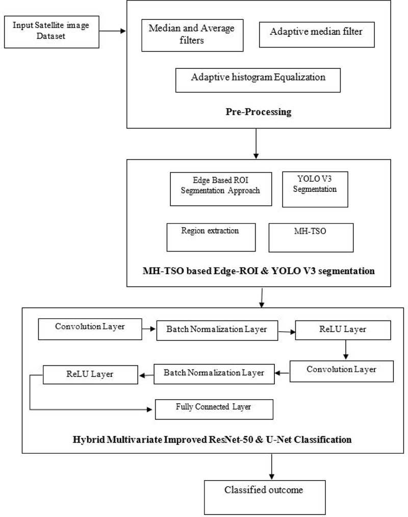
Figure 1: Overall flow depiction of suggested scheme.
A target recognition model was presented in [15] that has some additional features that were dependent on CNN architecture with features for the remote sensing images. The suggested CNN technique consists of two steps. First is the extraction of features using max-pool and average pooling functions. Then training was performed with fully-connected layers. The suggested technique attains high recognition accuracy of about 94.38% for about 10 classes in the military target’s detection in the MSTAR dataset.
An automatic target detection of satellite images was projected in [16] with the use of two kinds of machine learning schemes which offers better classification accuracy. Primarily, the support vector machine (SVM) was utilized along with a proper optimization approach for developing a set of local features. Then, the novel structure of CNN was implemented and both methods were analyzed with practical aspects.
A new technique of target recognition was suggested in [17] for the purpose of target recognition using CNN. Initially, from MSTAR datasets the targeted images are classified with the use of CNN. Then, the features were extracted from CNN output from convolution layer from which the position of targets were located in the image with the use of clustering and sampling approach. The suggested technique not only comprehends detection of target efficiently but also offers contented accuracy similarly in classifier function.
A multi feature-based convolution neural network (MFCNN) was presented in [18] for the recognition of targets from input image. First, from the satellite images the features were extracted. Then it was aggregated by the complementary relations as a single column vector. Finally, the target was identified with the use of fully connected networks. The suggested method has the advantage that it has the capability to recognize targets of MSTAR dataset images accurately on comparing other existing methods and was capable of offering information regarding the pose.
A speckle-noise-invariant CNN was projected in [19] along with regularization for decreasing the noise present in image and so as to recognize targets from images. Image despeckling was performed using Lee sigma filter to extract features. Then, the targets were recognized from the despeckled images using CNN training. The suggested CNN along with approach of regularization improves the recognition accuracy on relating traditional methods.
A recurrent neural network (RNN) [20] was proposed for automatic target recognition (ATR). Once electromagnetic waves from a radar incident on the targets, scattering of the incident energy might rise and this scattered signal was recognized as a target radar signature. The anticipated RNN based technique offers an accuracy of 93% in terms of classification.
Remote sensing image classification was a typical application [21]. In an attempt to augment the remote sensing image classifier outcomes, multiple classifiers combinations were utilized for classifying the Landsat-8 Operational Land Imager (Landsat-8 OLI) images. Few classifier techniques and algorithms combinations were scrutinized. The combined classifier encompassing of five classifiers adherent was made. The consequences of member in both classifiers were evaluated. The voting strategy was examined to take part the classification consequences of classifier member. The results exemplifies that the classifiers have unrelated performances and the grouping of several classifiers brings enhanced outcome on comparing the single classifier, thereby this approach conquers overall higher accuracy of classification. An approach was supported in [22] regrading the flexible multiple-features hashing learning context which is meant for LSRSIR which took several features that were balancing as an input which acquires the function of feature mapping hybrid approach [23].
A pre-trained convolution neural network (CNN) was presented in [24] for ATR. The main shortcoming of ATR was that there was an availability of only limited datasets for training purposes and for this reason a deep learning model was employed. The projected scheme was dependent on employing a pre-trained CNN specifically AlexNet which was employed for feature extraction and after which the output features were trained using multiclass SVM classifier. The pre-trained network proposed offers an accuracy of about 99.4% for three targeted modules or classes.
An approach in [25] aims at tackling problems associated with ATR. The suggested scheme depends on the approach of transfer learning at which three varied CNN that were pretrained are employed as feature extractors along with the integration of SVM. In this approach, the suggested classifier models are AlexNet, Google Net, and VGG16. On analyzing the performance, those three CNNs were capable of competing the issues of ATR at which AlexNet offers accuracy of about 99.27%.
A comparison was made in [26] among pre-trained CNN and SVM for the recognition of target so as to extract features and it was found that CNN offers better accuracy than others. Since there were several techniques employed for the classification and recognition of target in satellite images, there is a need to enhance the accuracy level so as to attain better detection of targets.
III. PROPOSED WORK
Our proposed methodology is explained briefly in this section. The overall flow depiction of the suggested method is given in Fig. 1. A deep learning-based model is implemented in this work for the better recognition and classification of targets from the satellite images. Initially, the input image is preprocessed, segmented using Edge-ROI and YOLO v3 based segmentation at which the parameter is tuned by means of multi-heuristic tuna swarm optimization (MH-TSO) approach and was classified using hybrid multivariate improved residual network (ResNet) and U-Net classifier approach. The stage of Edge-ROI segmentation and YOLO v3 based segmentation is employed to extract regions. The preprocessing is supported using median, average filtering along with adaptive histogram equalization. A scheme of deep learning-based multivariate improved residual neural network for classification of satellite images is proposed.
A. Input image pre-processing
Once the input image is collected, preprocessing is the initial and significant step for classifying satellite images. The process of preprocessing is employed so as to confirm the accessibility and reliability of the input images. In this, every step is significant since it aims at reducing the workload of further functions. This preprocessing step is carried out with the use of filters, histogram equalization techniques for detecting unintentional errors which could impair the capability of artifacts to prevent noise in the image. The abnormality areas are extracted from the satellite images. A non-linear filtering system is termed as adaptive median filter that is most widely employed in eradicating noise present in image. The major benefit of this noise reduction process is that it is an archetypal step to yield better performance. Figure 2 shows the input image and noisy input image.
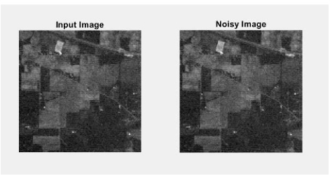
Figure 2: Input image and noisy image.
This is the preliminary step of the suggested approach which eliminates background noises. Salt and pepper along with Gaussian noise will be present in satellite images which should be removed to attain a high-quality image. The preprocessing step is accomplished to delete these redundant noises in the image. Unnecessary errors are identified by employing filtering and histogram techniques. In this phase, the extracted noise is filtered through an adaptive filtering technique which is employed for the purpose of isolating noise from the image and it acts as a non-linear optical filterer. A typical approach for noise eradication is carried for improving the efficiency of the system and thus to augment the image contrast. Gaussian noise will be rectified by means of adaptive Wiener filter (AWF). The filtering process aids in offering bright and clear images. The use of this AWF aids in offering smooth and less variant images.
A non-linear spatial filter that is most widely employed is the median filter which in turn replaces the pixel values by the gray level medians in the desired neighborhood of that pixel. The adaptive median filter is a kind of statistic order since their response depends on pixel ranking of the image area covered by means of a filter. It is widely employed since this offers reduction of noise by blurring fewer edges. This noise reducing effect depends on two major factors: number of noise pixels involved in the computation of median and the spatial extent of their neighborhood.
Normally, for augmenting the consistency of the system, histograms are equalized. Histogram equalization is regarded as the computerized process of enhancing the image contrast. The most significant values of sensitivity are increased by this. The spectrum strength of the image is widened. After this process the average image contrast is augmented.
Let us assume q signifies the normalized histograms for intensities that are all possible. This can be expressed as:
| (1) |
where x 0, 1…, x-1.
Thus, the histogram equalized image is signified as:
| (2) |
Here, base signifies the adjacent integer and is equivalent in transforming the intensity of pixel. The probability distribution function PDF of this is expressed as:
| (3) |
The probability distributed standardization function can be signified as .
At the time of preprocessing, the grayscale channel is blocked. Usually, the poor contrast image appears with satellite objects. The process of preprocessing is employed for augmenting the greyscale channel’s contrast. Histogram equalization is a technique employed for escalating the image contrast and is followed by growing usual values of intensity effectively. This is expressed as:
| (4) |
This approach not only enhances image quality but also augments the performance of the system.
B. Edge-ROI and YOLO-V3 based segmentation approach for extraction of regions
Detection of boundaries in the image border is carried out in this step. Understanding the characteristics of image edge detection is the most crucial step since edges comprise significant and necessary information and features. An image size is reduced considerably after filtering process so as to retain indispensable functional properties of an image. Typically, edge detection is employed for extracting boundaries or edges of image and is extensively used in image segmentation process. In the initial derivatives of the image, edges are sensed by gradient approach at which the edges are minimal. For this reason, suitable thresholding is employed to attain sharp edge isolation. Region of Interest (RoI) is evaluated that is divided to compute dimensions at which target edges will be extracted from the desired region. Figures 3 and 4 show the segmented image at frame 0 and frame 30.
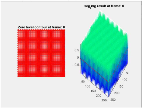
Figure 3: Segmented image at frame 0.
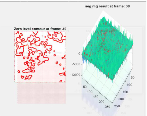
Figure 4: Segmented image at frame 30.
The approach of segmentation determines whether the neighbor of the region should be included or not. A regional mechanism is employed for combining the sub regions or pixels as bordered areas. A pixel aggregation is the simpler one which begins with collection of seed point from grown regions once the neighbor pixel has same features which will be attached to every seed points. This is expressed as:
| (5) |
where refers to region of interest segmentation, velocity gradient is represented by , denotes the lower and higher pixel values of image, M signifies pixel numbers block of the image, denotes the image’s spatial size, signifies the image’s frequency coefficient, denotes the pixel distance.
The image frequency co-efficient is thus tuned by means of MH-TSO technique. The optimal features selection thus enhances the segmentation outcome. The optimal range of features are thus selected using MH-TSO algorithm.
Initial step is the spiral foraging model at which tuna will swim once it is nursed thus forming spiral ones for derivation of shallow water feed which is simply attacked. Next step is the parabolic foraging at which corresponding tuna thus swims subsequently making a parabola shape for enclosure of its prey. Using these techniques, tuna forage successfully. Mathematical modeling of this optimization technique is:
| (5) |
where refers to the ith initial individual, ub and lb are the upper and lower boundaries of search space, NP refers to the number of tuna population and rand signifies the random vector which is uniformly distributed and ranges from 0 to 1.
The anticipated mathematical modelling of spiral foraging is:
| (8) |
where signifies the reference point which is randomly generated at search space. Specifically, typical algorithms that are metaheuristic might transmit wide global exploration at a previous stage and then transfer to exact local exploitation slowly.
The anticipated mathematical modelling of parabolic foraging is:
| (12) |
where TF refers to the random number having the value 1 or -1. The tuna hunt cooperates over two approaches of foraging and identifies the prey.
Deep learning-based YOLO v3 is employed for the segmentation process to get accurate segmented regions. Typical versions of YOLO do not have localization error resolution. The newer version of this was not capable of identifying the smaller objects. YOLO v3 is designed for handling the existing limitations and thus offers an enhanced output during testing phase. Version 3 offers enhanced outcome for small size objects. It does not offer precise output for huge objects. The YOLO v3 architecture depends on Darknet-53 strategy that utilizes 33 and 11 convolutional filters having scarce shortcut connections with convolution layers which is twice as fast as ResNet-152. YOLO v3 is stimulated through Feature Pyramid Network (FPN) that covers heuristics like up-sampling, residual blocks and skip connections. It provides Darknet53 as a ground network, that integrates 53 more layers to detect objects more easily. Like FPN, YOLO v3 utilizes 11 convolution to detect objects. Feature maps are produced at three different levels. It down samples the input by a factor of varied levels. On employing a stride of 32, in the the result tensor is feature map which is used to detect with the help of 11 . After applying a stride of 16, the detection is done after the 94th layer. Adding some convolutions on the 79th layer is done and then combined with 61st layer on to get a 26x26 feature map. After applying a stride of 8, detection is made in the 106th layer with the help of feature map. Some convolutions are combined to 91st layer and then integrating with the 36th layer with the help of , the down-sampled feature maps are integrated with the up-sampled maps at various locations to get fine grained features to detect the smaller objects of different sizes. The varied feature maps 5252, 2626, and 1313 are employed for detecting huge, medium, and smaller objects correspondingly.
C. Classification using hybrid multivariate improved ResNet and U-Net classification
A ResNet and U-Net classifier is employed in this section after the segmentation process. The satellite image is recognized and is classified so as to recognize areas of vegetative lands from the input satellite images. This is the method employed for pre-trained convolution. CNN permits the valuation of inconsistencies among one or two objective variable quantity and one or both of them. The hybrid multivariate improved residual network and U-Net classifier offers a likelihood and the statistical distributions are usable. First, CNN reads the input thereby performing a resizing operation by measuring class likelihoods of validation phase. CNN in scrips a substantial development in the analysis and identification of images.
A hybrid multivariate improved ResNet and U-Net classifier is well-organized in the following layer forms: Convolution layers, Pooling layers, ReLU layers, Fully connected layers. This has predetermined pre-processing procedures, taking into consideration other images for classification purposes. This hybrid multivariate improved ResNet and U-Net classifier is employed for several determinations in many fields.
Hyperparameter selection is done manually or automatically. In this model, manual selection is carried out due to the highly complex nature and computational cost of the automatic models. The dataset is evaluated by the suggested ResNet classifier model by employing an optimization approach. The hyperparameters that are needed for estimating the model parameters are hidden layers, activation functions, data augmentation, kernel size, padding, and stride. The hyperparameters that are employed for controlling the training algorithm behavior are learning rate, batch size, momentum, and number of epochs. In this model, batch normalization is employed after the convolution layer and before the activation function. This technique is employed with suitable optimizer like stochastic gradient descent (SGD) optimizers at which learning rate and weight decay of ResNet system provides an improved stage of final trainings and validation accuracy that overcomes issue of overfitting thereby reducing the computational complexity of training process. Hyperparameter tuning parameters for the presented ResNet system are shown in Table 1.
Table 1: Hyperparameter tuning parameters for the presented ResNet system
| Hyperparameter | Value |
| Batch size | 128 |
| Epochs | 200 |
| Rate of learning | 0.04 |
| Momentum | 0.9 |
| Weight decay | 5e-4 |
| Drop out fully connected | 50% |
| Optimizer | Stochastic gradient descent |
| Activation function | ReLU |
This classifier makes it possible to estimate the inconsistency among one or more of the variables. The multipath improved ResNet classifier estimates the probabilities. In this method, the classifier will initially calculate, redistribute, and then interpret the class probability of the image:
| (13) |
where Fea signifies the feature, p denotes the pointed feature. The following expressions are made:
| (14) | ||
| (15) |
where represents the features classified. The CNN classification was concluded as:
| (16) |
where L is the empirical constant.
U-Net architecture comprises a constricting growing lower side and upper side. The constricting side consist of two 33 convolution layers intended for the iterative model. These two convolutional layers are the modified U-Net layer, and the down sampling layer has a function of 22 extreme pooling with two steps. The count of channel attributes becomes twice in every down sampling step. At the growing path, every step comprises of upsampling attributes that are tracked through a 22 convolution layer which in turn halves the counts of attributes. Finally, the block of 11 convolution is thus employed for mapping the sets of 64 attributes vectors for the class number. Moreover, normalization is added to the input layer at the actual U-Net structure. It was assured that input data dispersion at each layer is stable at the time of input normalization. The entire data is utilized to learn the full convolution through the computation of feed forward and the back propagation process.
Classification is performed using hybrid multi-variate improved ResNet and U-Net classifier. As a result of the classification process, vegetative land covers are identified effectively. The performance investigation of the anticipated system is revealed in the performance analysis section.
IV. PERFORMANCE ANALYSIS
This section is the presentation of comprehensive elucidation of the performance analysis of the projected system. The proposed methodology performance is enumerated by calculating several metrics of performance including accuracy, specificity, precision, recall, F-measure and sensitivity.
A. Accuracy
Accuracy Ai depends on the number of targets that are classified correctly and is evaluated by:
| (17) |
where TP is True Positive, TN is True Negative, FP is False Positive, FN is False Negative.
B. Recall sensitivity
Sensitivity measures how many positives are correctly identified as positives and is defined as
Specificity measures how many non-targets are correctly identified as non-targets and is defined as
| (19) |
D. Precision
Precision is defined as the ratio of the number targets that are classified to the number of targets present in an image
| (20) |
E. F-Measure
F-Measure is obtained by combining precision and recall
| (21) |
The datasets employed in this work are listed below.
F. Dataset description
This is the segmentation of hyperspectral image dataset. The input source data encompasses of hyperspectral bands over a sole scenery in Indiana, USA (Indian Pines) dataset that has pixels of about 145145. In support of each pixel, data set encompasses of bands with spectral reflectance of around 220 which indicates several portions of electromagnetic spectrum in the range of wavelength 0.42.510-6.
Denoted as the dataset of hyperspectral image which is gathered through 224-band AVIRIS sensor over the Salinas Valley, California, and is characterized over high spatial resolution (about 3.7-meter pixels). The enclosed area encompasses of 512 lines having the sample of around 217, and the water absorption bands of about 20 were being discarded. This image is being accessible as the data of senor radiance and it includes bare soils, vegetables, and vineyards fields. The ground truth Salinas encompasses of 16 classes.
The dataset Pavia University is a hyperspectral image type which is accumulated by a labelled sensor as a system of reflective optics imaging spectrometer (ROSIS-3) over Pavia City, Italy. It encompasses of pixels 610340 by 115 spectral bands. The image is thus divided as nine classes having total labelled samples of about 42,776, with trees, meadows, gravel, bitumen, asphalt, bare soil, brick, metal sheet, and shadow.
G. Performance analysis of suggested system
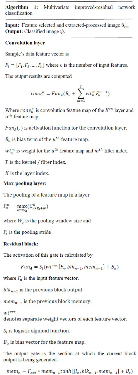
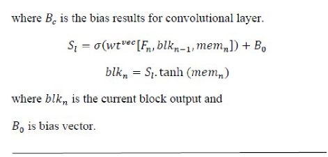
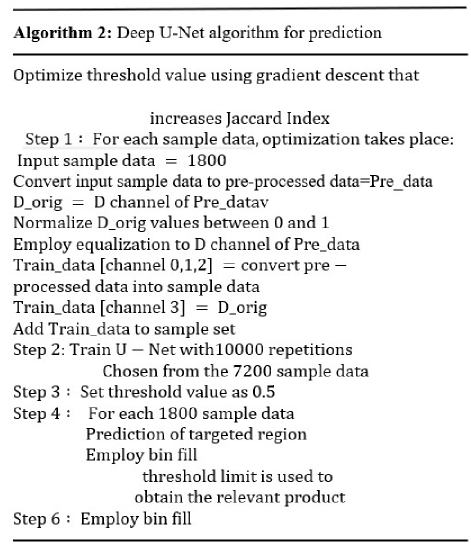
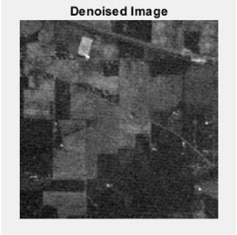
Figure 5: Denoised image.
Performance assessment of the anticipated result is revealed in Fig. 5. This shows the denoising process effect on the input image. Likewise, Fig. 6 indicates the segmentation outcome obtained as a result of the effective segmentation process by varying the level of iterations. The range of iteration set are 100, 200, and 500.
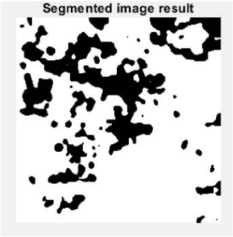
Figure 6: Segmented outcome.
The segmented outcome with various iteration values (100, 200 and 500) is shown. Figure 7 is the segmented outcome attained for 100 iterations. Figure 8 is the segmented outcome attained for 200 iterations. Figure 9 is the segmented outcome for 500 iterations.
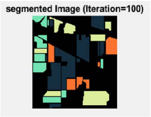
Figure 7: Segmented image at iteration 100.
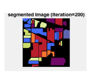
Figure 8: Segmented image at iteration 200.
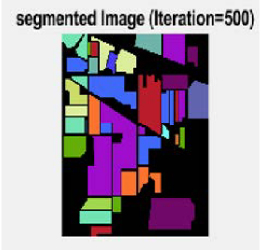
Figure 9: Segmented image at iteration 500.
Classified outcomes are illustrated in Fig. 10 which is assessed for the dataset Salinas. The identified and classified regions from the satellite image Salinas dataset is revealed. Each color signifies one parameter or area of vegetative land categorization. The categorization is labelled in Fig. 10 for clarity.
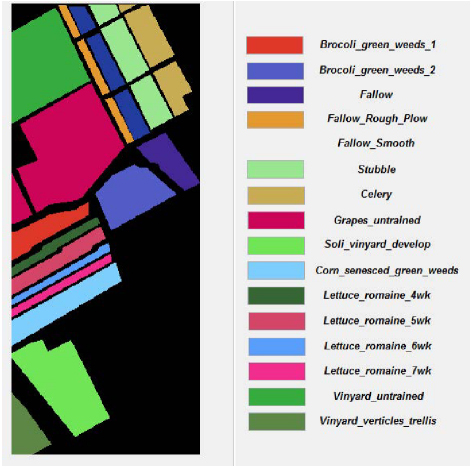
Figure 10: Classified outcomes for Salinas dataset.
The portrayal of classified consequence for Pavia University dataset is projected in Fig. 11. The recognized and classified regions from the satellite image Pavia University dataset are exposed. Each color indicates one parameter or area of different vegetative land category. The categorization is labelled in Fig. 11 for clarity.
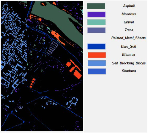
Figure 11: Classified outcomes for Pavia University dataset.
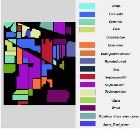
Figure 12: Classified outcomes for Indian Pines dataset.
The representation of classified result for Indian Pines dataset is given in Fig. 12. The classified and recognized regions from the satellite image Indian Pines dataset are given. Each color implies one parameter or area of vegetative land categorization. The categorization is labelled in Fig. 12 for clarity.
Table 2: Performance analysis of proposed system error measure
| Measure | Proposed Method |
| Peak signal to noise ratio (PSNR) | 46.4019 |
| Mean Square Error (MSE) | 1.2202 |
| Structure Similarity Index (SSIM) | 0.999 |
| Normalized Cross Correlation (NCC) | 1.003 |
| Image Enhancement Factor (IEF) | 0.9717 |
Table 2 illustrates performance investigation of anticipated methodology in terms of PSNR, SSIM, MSE, NCC and IEF.
H. Comparative analysis of proposed system
The classifier function is estimated and the outcomes for each dataset taken are given and the outcome is compared with existing algorithms for exposing the efficiency of proposed system. Table 3 shows the Salinas dataset performance analysis. The epochs are varied and the activation function is increased to estimate the outcomes of proposed system classifier.
Table 3: Salinas dataset performance analysis
| Salinas Dataset | ||||
| Epochs | 50 | 150 | 250 | 350 |
| Activation Function | ||||
| Tanh | 98.75 | 98.16 | 99.32 | 99.78 |
| Leaky ReLU | 97.12 | 97.28 | 97.34 | 98.91 |
| ReLU | 96.27 | 96.39 | 96.51 | 96.36 |
Table 4 shows the Pavia University dataset performance analysis. The epochs are varied and the activation function is increased to estimate the outcomes of proposed system classifier.
Table 4: Pavia University dataset performance analysis
| Pavia University Dataset | ||||
| Epochs | 50 | 150 | 250 | 350 |
| Activation Function | ||||
| Tanh | 96.24 | 96.75 | 97.36 | 97.28 |
| Leaky ReLU | 95.87 | 95.48 | 95.37 | 96.71 |
| ReLU | 94.25 | 94.58 | 94.68 | 94.12 |
Table 5: Indian Pines dataset performance analysis
| Indian Pines Dataset | ||||
| Epochs | 50 | 150 | 250 | 350 |
| Activation Function | ||||
| Tanh | 91.72 | 91.57 | 92.38 | 92.66 |
| Leaky ReLU | 90.28 | 91.24 | 92.34 | 93.51 |
| ReLU | 91.45 | 92.35 | 92.68 | 93.11 |
Table 5 shows the Indian Pines dataset performance analysis. The epochs are varied and the activation function is increased to estimate the outcomes of proposed system classifier.
Table 6: Comparative analysis of proposed classifier outcome
| Measures | Deep CNN | VGG-16 | ResNet-50 | Hybrid Multivariate Improved ResNet-50 and U-Net |
| Accuracy | 84.6579 | 87.9083 | 91.1588 | 96.0345 |
| Sensitivity | 5.6000 | 7.0000 | 9.3333 | 18.6667 |
| Specificity | 100 | 100 | 100 | 100 |
| Precision | 100 | 100 | 100 | 100 |
| Recall | 5.6000 | 7.0000 | 9.3333 | 18.6667 |
| F-Measure | 0.1061 | 0.1308 | 0.1707 | 0.3146 |
Table 6 shows the comparative analysis of proposed system classifier result. The performance of projected algorithm is related with prevailing performances like Deep CNN, VGG-16, and ResNet-50 to demonstrate the effectiveness of anticipated mechanism hybrid multivariate improved ResNet-50 and U-Net classifier. The classifier’s elapsed time is 54.064668 sec, OA (total accuracy) is 72.91%, AA (average accuracy is 89.83%), and kappa value is 0.684.
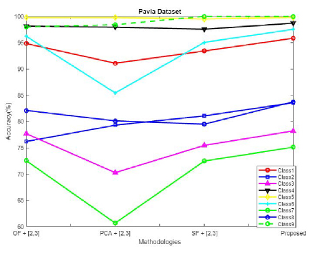
Figure 13: Comparative analysis of accuracy for Pavia University dataset.
The performance of projected algorithm is compared with existing techniques like OF (original spectral feature), PCA (principle component analysis), and SF (sparse feature) [27] in Fig. 13 to demonstrate the effectiveness of anticipated mechanism for varied classes in terms of accuracy for Pavia University dataset.
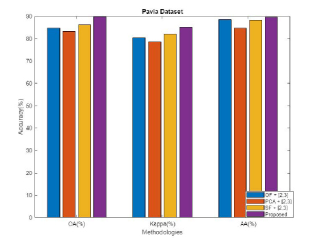
Figure 14: Comparative analysis for Pavia University dataset in terms of OA, kappa, and AA.
The performance of the projected algorithm is compared with existing techniques like OF, PCA, and SF in Fig. 14 to demonstrate the effectiveness of the anticipated mechanism for varied classes in terms of OA, kappa, and AA for Pavia University dataset.
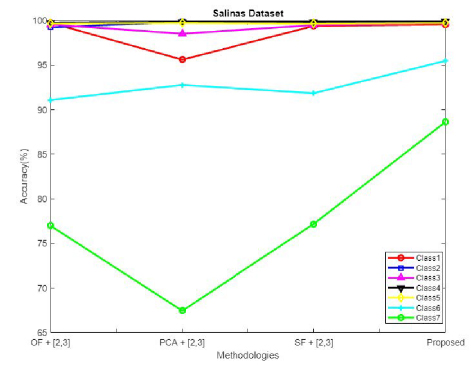
Figure 15: Comparative analysis of accuracy for Salinas dataset.
The performance of the projected algorithm is compared with existing techniques like OF (original spectral feature), PCA (principle component analysis), and SF (sparse feature) in Fig. 15 to demonstrate the effectiveness of the anticipated mechanism for varied classes in terms of accuracy for the Salinas dataset.
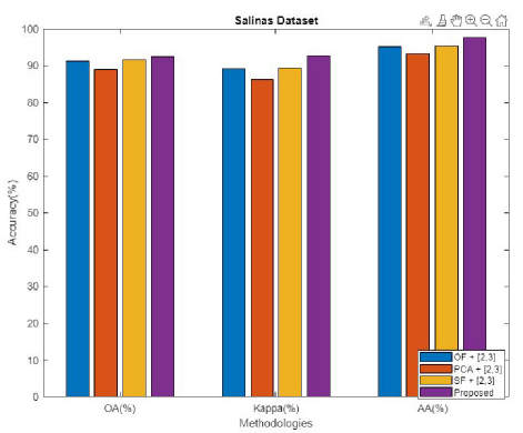
Figure 16: Comparative analysis for Salinas dataset in terms of OA, kappa, and AA.
The performance of the projected algorithm is compared with existing techniques like OF, PCA, and SF in Fig. 16 to demonstrate the effectiveness of the anticipated mechanism in terms of OA, kappa, and AA for Salinas dataset.
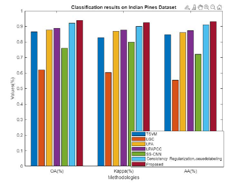
Figure 17: Comparative analysis for Indian Pines dataset in terms of OA, kappa, and AA.
The performance of the projected algorithm is compared with existing techniques [28] like TSVM, LGC, LPA, LPACC, SS-CNN, consistency regularization and pseudo-labelling in Fig. 17 to demonstrate the effectiveness of the anticipated mechanism in terms of OA, kappa, and AA for Indian Pines dataset.
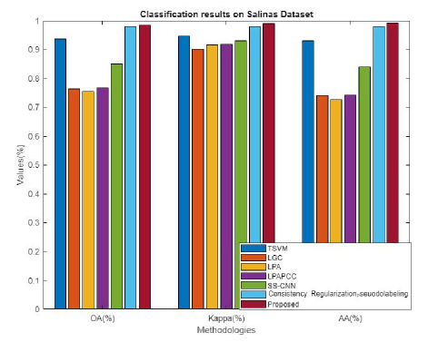
Figure 18: Comparative analysis for Salinas dataset in terms of OA, kappa, and AA.
The performance of the projected algorithm is compared with existing techniques like TSVM, LGC, LPA, LPACC, SS-CNN, consistency regularization, and pseudo-labelling in Fig. 18 to demonstrate the effectiveness of the anticipated mechanism in terms of OA, kappa, and AA for Salinas dataset.
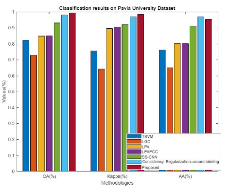
Figure 19: Comparative analysis for Pavia University dataset in terms of OA, kappa, and AA.
The performance of the projected algorithm is compared with existing techniques like TSVM, LGC, LPA, LPACC, SS-CNN, consistency regularization, and pseudo-labelling in Fig. 19 to demonstrate the effectiveness of the anticipated mechanism in terms of OA, kappa, and AA for Pavia University dataset.
Table 7: Accuracy comparison with existing models
| Model | Accuracy |
| Deep CNN | 88.412 |
| VGG-16 | 90.9150 |
| ResNet-50 | 92.5727 |
| MS-RPNet | 99.6500 |
| MFFCG | 98.9400 |
| Proposed | 99.8050 |
The accuracy of the existing model is compared with the proposed accuracy in Table 7, which shows enhancement over other compared models [29,30]. The accuracy of the proposed model is attained as 99.8050%.
Table 8: Performance comparison of different models on Indian Pines dataset
| Metrics | MS-RPNet | MFFCG-2 | Proposed |
| OA (%) | 98.8700 | 94.2500 | 99.3800 |
| AA (%) | NA | 93.9900 | 99.0600 |
| kappa (%) | 98.0500 | 93.2900 | 99.7800 |
Table 8 shows the performance comparison of various models on the Indian Pines dataset. The metrics analyzed are OA, AA, and kappa for proposed and existing schemes MS-RPNet and MFFCG-2 [29,30]. The proposed model shows the following results: OA99.38%, AA99.06%, and kappa99.78%, which is higher than existing values.
Table 9: Performance comparison of different models on Pavia University dataset
| Metrics | MS-RPNet | MFFCG-2 | Proposed |
| OA (%) | 99.7600 | 90.3400 | 99.8700 |
| AA (%) | NA | 94.1400 | 98.8600 |
| kappa (%) | 99.6800 | 93.5200 | 99.7300 |
Table 9 shows the performance comparison of various models on the Pavia University dataset. The metrics analyzed are OA, AA, and kappa for proposed and existing schemes MS-RPNet and MFFCG-2. The proposed model shows the following results: OA99.87%, AA99.86%, and kappa99.73%, which is higher than existing values.
Table 10: Performance comparison of different models on Salinas dataset
| Metric | MFFCG-2 | Proposed |
| OA (%) | 87.1700 | 98.6700 |
| AA (%) | 86.4900 | 99.0500 |
| kappa (%) | 85.1600 | 99.7100 |
Table 10 shows the performance comparison of various models on the Salinas dataset. The metrics analyzed are OA, AA, and kappa for proposed and existing scheme MFFCG-2. The proposed model shows the following results: OA98.67%, AA99.05%, and kappa=99.71%, which is higher than existing values. From analysis, it was obvious that the proposed model shows enhancement over other existing models.
V. CONCLUSION
In this approach, a deep learning-based automated technique for the detection, segmentation, and classification of satellite images was carried out. Initially, the input image was preprocessed, segmented using Edge-ROI and YOLO v3 model at which parameters are tuned by means of multi-heuristic tuna swarm optimization (MH-TSO), and was classified using hybrid multivariate improved residual network and U-Net classifier approach. The analysis was compared with traditional methods to validate the effectiveness of the proposed scheme. The proposed technique performance is estimated for three kinds of dataset: Salinas, Pavia University, and Indian Pines satellite image datasets. The analysis shows that the proposed system offers better rate of recall, precision, and F-measure than existing techniques. The outcomes show that the designed method overcomes the issues of existing satellite image classification methods through classifying the satellite image in an effective manner. In future, this work can be extended by integrating attention mechanisms or transformer based models to further improve feature representation, and also by applying this framework to other domains like urban planning, agricultural monitoring, and disaster assessment for evaluating their broad applicability.
REFERENCES
[1] X. Zhang and J. Xiang, “Moving object detection in video satellite image based on deep learning,” in Proc. SPIE LIDAR Imaging Detection and Target Recognition, Xi’an, China, vol. 10605, p. 106054H, 2017.
[2] F. A. Mianji, Y. Gu, Y. Zhang, and J. Zhang, “Enhanced self-training superresolution mapping technique for hyperspectral imagery,” IEEE Geoscience and Remote Sensing Letters, vol. 8, no. 4, pp. 671-675, 2011.
[3] M. J. Khan, H. S. Khan, A. Yousaf, K. Khurshid, and A. J. I. A. Abbas, “Modern trends in hyperspectral image analysis: A review,” IEEE Access, vol. 6, pp. 14118-14129, 2018.
[4] J. Chen and A. Zipf, “Deep learning with satellite images and volunteered geographic information,” in Geospatial Data Science Techniques and Applications, J. Chen and A. Zipf, Eds. Boca Raton, FL: CRC Press, p. 63, 2017.
[5] C. Avolio, M. Á. M. Armenta, A. J. Lucena, M. J. F. Suarez, P. V. Martin-Mateo, and F. L. González, “Automatic recognition of targets on very high resolution SAR images,” in 2017 IEEE International Geoscience and Remote Sensing Symposium (IGARSS), pp. 2271-2274, 2017.
[6] R. J. Soldin, “SAR target recognition with deep learning,” in 2018 IEEE Applied Imagery Pattern Recognition Workshop (AIPR), Washington, DC, USA, pp. 1-8, 2018.
[7] Y. E. García-Vera, A. Polochè-Arango, C. A. Mendivelso-Fajardo, and F. J. Gutiérrez-Bernal, “Hyperspectral image analysis and machine learning techniques for crop disease detection and identification: A review,” Sustainability, vol. 16, no. 14, p. 6064, 2024.
[8] P. Ilamathi and S. Chidambaram, “Integration of hyperspectral imaging and deep learning for sustainable mangrove management and sustainable development goals assessment,” Wetlands, vol. 45, no. 9, 2025.
[9] N. Dahiya, G. Singh, S. Singh, and V. Sood, “Crop land assessment with deep neural network using hyperspectral satellite dataset,” in Hyperautomation in Precision Agriculture. Cambridge, MA, USA: Academic Press, pp. 159-167,2025.
[10] P. Sevugan, V. Rudhrakoti, T. H. Kim, M. Gunasekaran, S. Purushotham, and R. Chinthaginjala, “Class-aware feature attention-based semantic segmentation on hyperspectral images,” PLoS One, vol. 20, no. 2, p. e0309997, 2025.
[11] R. Luo, P. Lu, P. Chen, H. Wang, X. Zhang, and S. Yang, “Hyperspectral classification of ancient cultural remains using machine learning,” Remote Sensing Applications: Society and Environment, vol. 37, p. 101457, 2025.
[12] Q. Zhe, W. Gao, C. Zhang, G. Du, Y. Li, and D. Chen, “A hyperspectral classification method based on deep learning and dimension reduction for ground environmental monitoring,” IEEE Access, 2025.
[13] S. Chen, H. Wang, F. Xu, and Y.-Q. Jin, “Target classification using the deep convolutional networks for SAR images,” IEEE Transactions on Geoscience and Remote Sensing, vol. 54, no. 8, pp. 4806-4817, 2016.
[14] Z. Lin, K. Ji, M. Kang, X. Leng, and H. Zou, “Deep convolutional highway unit network for SAR target classification with limited labeled training data,” IEEE Geoscience and Remote Sensing Letters, vol. 14, no. 7, pp. 1091-1095, 2017.
[15] J. H. Cho and C. G. Park, “Multiple feature aggregation using convolutional neural networks for SAR image-based automatic target recognition,” IEEE Geoscience and Remote Sensing Letters, vol. 15, no. 12, pp. 1882-1886, 2018.
[16] I. Fedorchenko, A. Oliinyk, A. Stepanenko, T. Zaiko, S. Shylo, and A. Svyrydenko, “Development of the modified methods to train a neural network to solve the task on recognition of road users,” Eastern-European Journal of Enterprise Technologies, vol. 2, no. 9, pp. 46-55, 2019.
[17] H. He, S. Wang, D. Yang, and S. Wang, “SAR target recognition and unsupervised detection based on convolutional neural network,” in Proc. 2017 Chinese Automation Congress (CAC), pp. 435-438, 2017.
[18] I. M. Gorovyi and D. S. Sharapov, “Comparative analysis of convolutional neural networks and support vector machines for automatic target recognition,” in Proc. 2017 IEEE Microwaves, Radar and Remote Sensing Symposium (MRRS), pp. 63-66, 2017.
[19] Y. Kwak, W.-J. Song, and S.-E. Kim, “Speckle-noise-invariant convolutional neural network for SAR target recognition,” IEEE Geoscience and Remote Sensing Letters, vol. 16, no. 4, pp. 549-553, 2018.
[20] B. Sehgal, H. S. Shekhawat, and S. K. Jana, “Automatic target recognition using recurrent neural networks,” in Proc. 2019 Int. Conf. on Range Technology (ICORT), Chandipur, India, pp. 1-5, 2019.
[21] H. Shen, Y. Lin, Q. Tian, K. Xu, and J. Jiao, “A comparison of multiple classifier combinations using different voting-weights for remote sensing image classification,” International Journal of Remote Sensing, vol. 39, no. 11, pp. 3705-3722, 2018.
[22] D. Ye, Y. Li, C. Tao, X. Xie, and X. Wang, “Multiple feature hashing learning for large-scale remote sensing image retrieval,” ISPRS International Journal of Geo-Information, vol. 6, no. 11, p. 364, 2017.
[23] M. Häberle, M. Werner, and X. X. Zhu, “Geo-spatial text-mining from Twitter: A feature space analysis with a view toward building classification in urban regions,” European Journal of Remote Sensing, vol. 52, no. 2, pp. 2-11, 2019.
[24] M. Al Mufti, E. Al Hadhrami, B. Taha, and N. Werghi, “SAR automatic target recognition using transfer learning approach,” in Proc. 2018 Int. Conf. on Intelligent Autonomous Systems (ICoIAS), Singapore, pp. 1-4, 2018.
[25] M. Al Mufti, E. Al Hadhrami, B. Taha, and N. Werghi, “Using transfer learning technique for SAR automatic target recognition,” in Proc. SPIE Future Sensing Technologies, Tokyo, Japan, vol. 11197, p. 111970A, 2019.
[26] A. Khan, A. Sohail, U. Zahoora, and A. Qureshi, “A survey of the recent architectures of deep convolutional neural networks,” Artificial Intelligence Review, vol. 53, pp. 5455-5516, 2020.
[27] W. NanLan and Z. Xiaoyong, “Hyperspectral data classification algorithm considering spatial texture features,” Mathematical Problems in Engineering, vol. 2022, p. 901234, 2022.
[28] X. Hu, T. Zhou, and Y. Peng, “Semisupervised deep learning using consistency regularization and pseudolabels for hyperspectral image classification,” Journal of Applied Remote Sensing, vol. 16, no. 2, p. 026513, 2022.
[29] H. Chen, T. Wang, T. Chen, and W. Deng, “Hyperspectral image classification based on fusing S3-PCA, 2D-SSA and random patch network,” Remote Sensing, vol. 15, no. 13, p. 3402, 2023.
[30] U. A. Bhatti, M. Huang, H. Neira-Molina, S. Marjan, M. Baryalai, and H. Tang, “MFFCG: Multi feature fusion for hyperspectral image classification using graph attention network,” Expert Systems with Applications, vol. 229, p. 120496,2023.
BIOGRAPHIES

P. Pabitha Muthu is currently serving as an Assistant Professor in the Department of Computer Science and Engineering at Sethu Institute of Technology, located in Kariapatti, Virudhunagar District 626115, Tamil Nadu, India. She earned her undergraduate degree in Computer Science and Engineering from Pandian Saraswathi Yadav Engineering College. She completed her postgraduate studies in the same field at the same institution in 2014. Her research is focused on satellite image processing and wireless sensor networks.

S. Siva Ranjani is a Professor at Sethu Institute of Technology, Pulloor, Kariapatti Taluk, Virudhunagar District, India. She completed her post-graduation in Computer Science and Engineering from Kalasalingam University in 2007. She was awarded a Ph.D. in the same discipline in 2015, with her research focusing on Wireless Sensor Networks. Her areas of interest include data mining, wireless sensor networks, remote sensing, and image processing.
M. Manikandakumar is currently an Assistant Professor in the department of AIML and Data Science, Christ University, Kengeri Campus, Bangalore, India. He completed his post-graduation in Computer Science and Engineering in 2013 from Anna University, Chennai, where he completed the Ph.D in Information and Communication Engineering in 2023. He is currently an Assistant Professor in the department of AIML and Data Science, Christ University, Kengeri Campus, Bangalore. His research interests include data science, wireless networking, and machine learning, image processing and computer vision.
ACES JOURNAL, Vol. 40, No. 8, 679–693
doi: 10.13052/2024.ACES.J.400801
© 2025 River Publishers