Parameter Optimization of Electromagnetic Sensing and Driving Scheme of a Compact Falling-body Viscometer

Kun Zhang $^{1}$ , Hongbin Zhang $^{2}$ , Yuan Xue $^{3}$ , Jinyu Ma $^{2}$ , Jiqing Han $^{1}$ , and Xinjing Huang $^{2}$

¹Shandong Non-Metallic Materials Institute
Jinan 250031, China
zhangkun8185@163.com, qddxhjq@163.com

²State Key Laboratory of Precision Measurement Technology and Instruments
Tianjin University, Tianjin 300072, China
1360387520@qq.com, jinyu.ma@tju.edu.cn, huangxinjing@tju.edu.cn

³National Institute of Measurement and Testing Technology
Chengdu 610021, China
383622356@qq.com

Submitted On: July 3, 2024; Accepted On: September 9, 2024

ABSTRACT

In order to achieve automatic fast reset of the falling-body (FB) viscometer, and reduce the volume of the device and the amount of sample used, this paper proposes to use a single coil to reset the FB and use another single coil to measure the FB position. In this paper, the characterization ability of the sensing coil impedance to the FB position and its influencing factors, and the reset ability of the driving coil to the FB and its enhancement factors, are studied via electromagnetic finite element simulations and experiments. There is a linear zone between the FB position and the sensing coil impedance, with the slope being largest. The lower limit of the FB motion should be designed in this linear zone to accurately determine the moment when the FB reaches the lower limit point. Increase in the FB height, and in the number of turns of the sensing coil, and decrease in the wire diameter are beneficial to the FB positioning. There is a maximum force point when the FB approaches the driving coil, and the FB’s motion range needs to cover this point for reliable reset. Using iron plugs allows the FB to obtain greater electromagnetic attraction and ensure its successful reset. Experimental results show that the device requires only 1 mL of sample to measure liquid viscosity. For 9.5-1265 mPa $\cdot$ s dimethyl silicone oil, the average absolute value of the relative measurement error is 0.22% and the maximum value is 4.3%.

Index Terms: Electromagnetic coil, electromagnetic force, falling-body method, impedance measurement.

I. INTRODUCTION

Viscosity is an inherent physical property of fluid that reflects the friction between molecules when the fluid is subjected to external force [1]. Measuring the viscosity of a high-temperature and high-pressure liquid can assess the flow characteristics of the liquid, which is of great importance in the fields of oil and gas exploitation [2], coal liquefaction [3][4], the chemical industry and the operation of power equipment. At present, commonly used methods for measuring high-temperature and high-pressure liquids are the capillary method [5][6], the resonance string method [7][8], the rotation method [9][10] and the falling-body (FB) method.

Due to the small diameter of the capillary tube, the capillary viscometer has a high risk of clogging when measuring high-viscosity liquids. The resonant string viscometer necessitates the utilization of a long container in order to facilitate the vibration of the metal wire, thereby increasing the demand for liquid samples. The structure of the rotary viscometer is relatively complex and there is rotary transmission friction. The rotary viscometer requires a great number of components and has a large volume. It necessitates a considerable quantity of samples for measurement of liquids, which render it unsuitable for the viscosity measurement of expensive liquids.

Compared with the capillary method, the resonance string method and the rotation method, the FB method exhibits distinctive advantages. Its structure is simple, and it is easy to form a closed cavity to carry out viscosity measurements under high temperature and high pressure.

Development of the FB viscometer can be traced back to Bridgman [11][12] who used a falling cylinder to test the viscosity of 43 different fluids under high pressure. Bridgeman pointed out that the viscosity of the fluid is positively related to the falling time of the falling cylinder. The theory of measuring liquid viscosity using the FB method has been continuously improved. As the FB descends, the liquid is displaced, forcing it through the annular area between the tube wall and the FB. This displacement of the liquid creates considerable resistance to the FB movement. Lohrenz et al. [13] conducted a theoretical analysis of laminar flow in the ring of a FB viscometer and determined the calibration constant of the viscometer based on the analysis results. Ashare et al. [14] compared the difference in viscosity measurement using the FB method between non-Newtonian fluids and Newtonian fluids and gave an approximate expression for the viscosity of non-Newtonian fluids. Cristescu et al. [15]obtained the velocity profiles of liquid flow in open tubes and closed tubes, simplified the influence of various parameters of the FB on the fluid flow, obtained the formula for measuring the viscosity coefficient, and designed a FB viscometer with an ultrasonic transducer that measures the falling time of the FB. Gui et al. [16] obtained the numerical solution of the flow field around the cylindrical FB, determined the end correction factor, and gave the relevant equations for the end correction factor. Irving and Barlow [17] pointed out that when the diameter of the falling cylinder is less than 93% of the pipe diameter, the FB will fall eccentrically, resulting in unstable fall-time measurement. They therefore developed a high-pressure automatic falling cylinder viscometer using a solid cylinder and a FB with a central hole adapted to liquids of different viscosities. The falling time of the FB is measured by a series of detection coils on the viscometer tube.

In the measurement of viscosity of high-temperature and high-pressure liquids, the FB method has been applied often. Průša et al. [18] studied the measurement of viscosity of liquids of variable viscosity values with a FB viscometer and derived a modification of the classical formula for fluids with pressure-dependent viscosity. The systematic error introduced by the classical formula in measuring fluids with pressure-dependent viscosity is analyzed. Bair et al. [19][20] developed a compact and easy-to-operate viscometer using the FB method. Two concentric cylinders are used to form a pressure vessel. High temperature conditions are achieved by heating the air in the gap between the two cylinders. The inner cylinder and the plug are connected through threads to form a sealing device. The inner cylinder is connected to an external pressure-generating device to achieve high-pressure conditions. This device can be used to measure the viscosity of lubricants under high-temperature and high-pressure conditions of 1 GPa and 100 $^{\circ}$ C. Bair measured the viscosity of two compressor oils at 1.2 GPa using the same device and provided correlations between compressor oil viscosity and temperature as well as between compressor oil viscosity and pressure [20]. This correlation has broad applicability and can be generalized to other liquids. Harris [21] designed a FB viscometer to operate in the pressure range 0.1-400 MPa. A hollow cylinder with a hemispherical surface was used as the FB, and it was verified through experimental data that the relationship between the calibration constant (A) of this shape of FB and the gap (c) between the FB and the cylinder conforms to the dependenceof A $\propto$ c $^{-}$ $^{3}$ .

When applying the FB method to measure the viscosity of high-temperature and high-pressure liquids, two problems need to be solved: the non-contact detection of the FB position and control of the FB reset for the next measurement.

The commonly used method for detecting the FB position is to construct a Wheatstone bridge using two sensing coils. When the FB passes through the two sensing coils, it will cause an imbalance of the bridge signal. The imbalance signal is then amplified and shaped in order to control the opening and closing of the timer. By measuring the time of the FB passing through the two sensing coils, the stable speed of the FB and the viscosity of the liquid can be calculated. Harris [21] developed a high-pressure FB viscometer using this method. Due to the need to distinguish the unbalanced signals of the two sensing coils, the inductance change of the two coils cannot be affected simultaneously during the falling process of the FB. Consequently, the distance between the two sensing coils exceeds 100 mm, which results in a significant range of motion for the FB, a long detection period and the necessity for a large amount of liquid sample. Seung-Ho Yang et al. [22][23]developed a non-contact position sensor based on the change of magnetic core position using a single detection coil, but not for the FB viscometer. When the movable magnetic core is inserted into the detection coil, the change of the coil impedance is measured to indicate the change of magnetic core position, and the factors affecting the linearity and sensitivity of the sensor are studied. Compared with the method of using two sensing coils to construct a Wheatstone bridge to detect the FB position, this method can make the device more compact by delicately designing the coil size and position. Wang [24] developed a high-pressure liquid viscosity test system based on the FB method. However, they do not provide a FB reset scheme and the system can only measure once. The high-pressure FB viscometer developed by Bair [19][20] and Schaschke et al. [25][26] uses the reset method of rotating the entire pressure vessel by 180 $^{\circ}$ , which requires a large space and a considerable length of time for detection. Due to the large range of movement of the FB, it cannot be reset by the electromagnetic force of a single driving coil.

In order to utilize the electromagnetic force of a single energized coil to achieve the FB reset, this paper proposes to use the impedance of a single sensing coil to detect the position of the FB to reduce the distance of travel of the FB, that is, to reduce the maximum distance between the driving coil and the FB. This can also reduce the length and volume of the sealing cavity. However, it is necessary to study the ability of a single sensing coil’s impedance to characterize the position of the FB and its influencing factors. It is necessary to study the ability of a single driving coil to attract and reset the FB as well as the factors that can enhance this ability.

In this paper, the electromagnetic drive and sensing device of the FB viscometer with a single sensing coil are studied and optimized. The device to be optimized comprises a closed stainless steel tube sealed by a plug within which an iron FB moves. Two coils are wound externally. One is the driving coil, which is used to control the reset motion of the FB after energization, and the other is the sensing coil, which is used to measure the positional change of the FB. Via finite element simulation, the number of turns, wire diameter and size of the sensing coil are optimized in order to improve the positioning ability of the FB. In order to enhance the reset force obtained by the FB, the distance between the two coils and the material of the plug are optimized. The feasibility of using the designed device to measure liquid viscosity is experimentally verified with dimethyl silicone oil of different viscosities.

II. MEASUREMENT PRINCIPLE

The developed FB viscometer device based on electromagnetic drive and sensing is shown in Fig. 1. It is expected that the designed device size will not exceed $Φ$ 40 mm*H80 mm. A stainless steel tube and a plug create a closed chamber filled with the liquid to be tested. The iron FB moves inside the closed cavity, and the movement range is the upper and lower limits of the closed cavity. The upper limit is the base of the plug, while the lower limit is the base of the chamber. The exterior of the steel tube is wrapped with two identical-sized coils serving distinct purposes: one for driving the FB to reset and the other for sensing the FBposition.

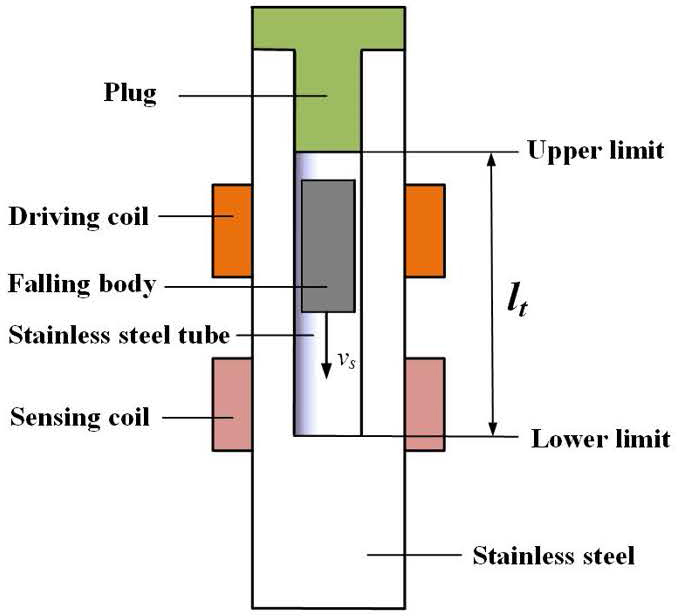
Figure 1: Schematic diagram of liquid viscosity measuring device.

The driving coil generates a magnetic field after being passed through current, which is used to attract the FB to move vertically upward until the FB reaches the upper limit to complete the reset of the FB. After the driving coil is powered off, the magnetic field disappears, and the FB falls coaxially in the tube under the action of gravity. When the FB reaches force balance under the combined action of gravity, buoyancy and viscous force that increases with speed, the FB’s speed reaches a stable value $v_{s}$ . The formula for calculating the liquid viscosity $η$ is presented in equation (1) [25]:

\begin{matrix} η = \frac{m g}{2 π v_{s} h_{1}} (1 - \frac{ρ_{l i q}}{ρ_{s}}) [\ln \frac{r_{2}}{r_{1}} - \frac{r_{2}^{2} - r_{1}^{2}}{r_{2}^{2} + r_{1}^{2}}] . \end{matrix}

(1)

In this equation, $r_{1}$ is the radius of the FB, h $_{1}$ is its length, $r_{2}$ is the radius of the tube within which the FB is falling, m is the mass of the FB, $ρ_{l i q}$ is the density of the liquid to be measured, and $ρ_{s}$ is the density of the FB. Replacing the stable speed $v_{s}$ of the FB with the moving distance $l_{t}$ of the FB divided by the falling time t, equation (1) can be rewritten as:

\begin{matrix} η = A t (1 - \frac{ρ_{l i q}}{ρ_{s}}) . \end{matrix}

(2)

A is the instrument coefficient, and its expression is:

\begin{matrix} A = \frac{m g [\ln \frac{r_{2}}{r_{1}} - \frac{r_{2}^{2} - r_{1}^{2}}{r_{2}^{2} + r_{1}^{2}}]}{2 π l_{t} l_{s}} . \end{matrix}

(3)

It can be seen from equation (2) that the liquid viscosity $η$ is proportional to the time t for the FB to fall over a fixed distance $l_{t}$ with a stable speed.

It was found through experimental observation that when the radius r $_{1}$ of the FB is close to the radius r $_{2}$ of the tube, the FB will quickly reach the stable speed $v_{s}$ in the falling initial stage. Reasonable design of r $_{1}$ and r $_{2}$ can make the acceleration process very short. The FB can be regarded as falling at a stable speed $v_{s}$ . By measuring the change in the impedance value of the sensing coil, the falling process of the FB is monitored and the time difference between the upper and lower limits of the FB movement is obtained. After calibrating the instrument coefficient A using a standard liquid with known viscosity, the liquid viscosity to be tested can be calculated according to equation (2) by measuring the ratio of the falling time t of the FB.

In order to achieve more accurate FB position detection, in section III an electromagnetic finite element simulation study is conducted to reveal the relationship between the FB position and the coil impedance with different coil parameters and FB parameters, and appropriate combination of parameters is provided. In order to increase the reset force and achieve more reliable FB reset, in section IV the law of electromagnetic force generated by the driving coil is simulated and studied, the upper and lower limit positions are designed, and the material of the plug is optimized.

III. SENSING SCHEME DESIGN

The finite element simulation software COMSOL was used to conduct a simulation study on the relationship between the position of the FB and the coil impedance. A 2D rotational axial symmetry model was constructed as shown in Fig. 2 (a). The stainless steel tube’s inner wall r ${}_{2}=$ 4 mm, thickness is 5 mm, length is 100 mm; the FB’s radius r ${}_{1}=$ 3.5 mm, height h ${}_{1}=$ 20 mm. The coil width WH $=$ 16 mm, the coil thickness is calculated by the coil width WH, the number of the coil turns N and the wire diameter d. The distance between section A-A and the center of the sensing coil is D ${}_{1}=$ 30 mm, the distance between the centers of the sensing coil and the driving coil is D ${}_{2}=$ 18 mm, the material of the FB is pure iron, the relative magnetic permeability is set to 300, and the electrical conductivity is set to 1.12 $\times$ 10 $^{7}$ S/m. The relative magnetic permeability of stainless steel is set to 1.2, and the electrical conductivity is set to 4.03 $\times$ 10 $^{6}$ S/m. The coil material is copper, the relative magnetic permeability is set to 1, and the electrical conductivity is set to 5.99 $\times$ 10 $^{7}$ S/m. The physical field is a magnetic field. The coil model is set to “uniform multi-turn”. The number of turns N $=$ 400, and it is the parameter to be swept. The wire diameter d $=$ 0.25 mm, and it is the parameter to be swept. The excitation voltage is set to 5 V. The mesh is set to “Physics Control Mesh” and the unit size is selected to “Ultra-Fine”. A frequency domain study is set and the frequency is set to 500 Hz. The position of the FB is described by the distance S from the center of the FB to the section A-A. In order to study the electromagnetic law between the FB position and the sensing coil regardless of travel distance limit, in the simulation in section III, the driving coil is set to “disabled”, the position of the FB is not restricted by upper and lower limits, and parameterized sweeping can be performed. A parametric sweeping on the FB position S is carried out, with a sweeping range of 0 $\sim$ 60 mm and a sweeping interval of 1 mm. Among them, the magnetic flux density distributions when S $=$ 0 mm, S $=$ 15 mm, and S $=$ 30 mm are shown in Figs. 2 (b-d).

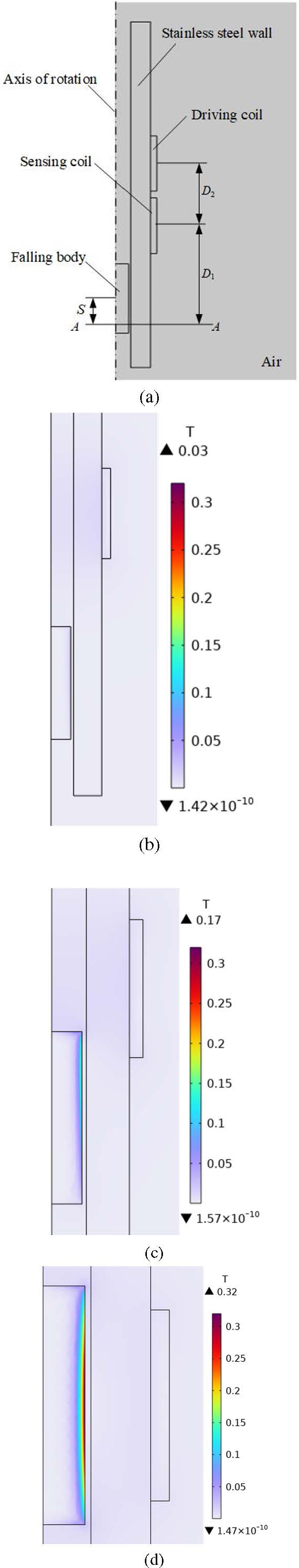
Figure 2: Magnetic flux density distributions generated by energizing the sensing coil when measuring the impedance of the sensing coil: (a) simulation model, (b) magnetic flux density distribution when S $=$ 0 mm, (c) magnetic flux density distribution when S $=$ 15 mm, and (d) magnetic flux density distribution when S $=$ 30 mm.

The sensing coil is energized and excited due to the need to measure its impedance. It can be observed from Figs. 2 (b-d) that the magnetic field generated is mainly concentrated on the surface of the FB. The FB at different locations will have a significant impact on the magnetic flux density distribution. When S $=$ 0 mm, the distance between the falling object and the sensing coil is far, and the magnetic field generated by the coil’s energization excitation has very little impact. When S $=$ 15 mm, as the distance between the FB and the sensing coil decreases, the magnetic field intensity on the FB increases and the magnetic induction lines become denser. When S $=$ 30 mm, the FB is located at the center of the sensing coil, and the magnetic field intensity on the falling object is the largest among the above three scenarios. As the FB moves toward the coil, it gathers magnetic flux, causing the inductance and impedance values of the coil to increase.

When measuring liquid viscosity by monitoring the impedance change of the sensing coil, the falling process of the FB can be monitored and the time difference of the FB falling from the upper limit to the lower limit can be obtained. The moment when the FB starts to fall at the upper limit is the moment when the driving coil is powered off, and the moment when the FB reaches the lower limit is the moment when the coil impedance value suddenly stops changing. Subsequently, parametric sweeping simulation will be used to optimize the number of the coil turns N, the wire diameter d, the length of the FB h $_{1}$ , the upper and lower limits of the FB, and the plug material of the closed tube, to ensure the accuracy of the falling time measurement and the reliability of reset.

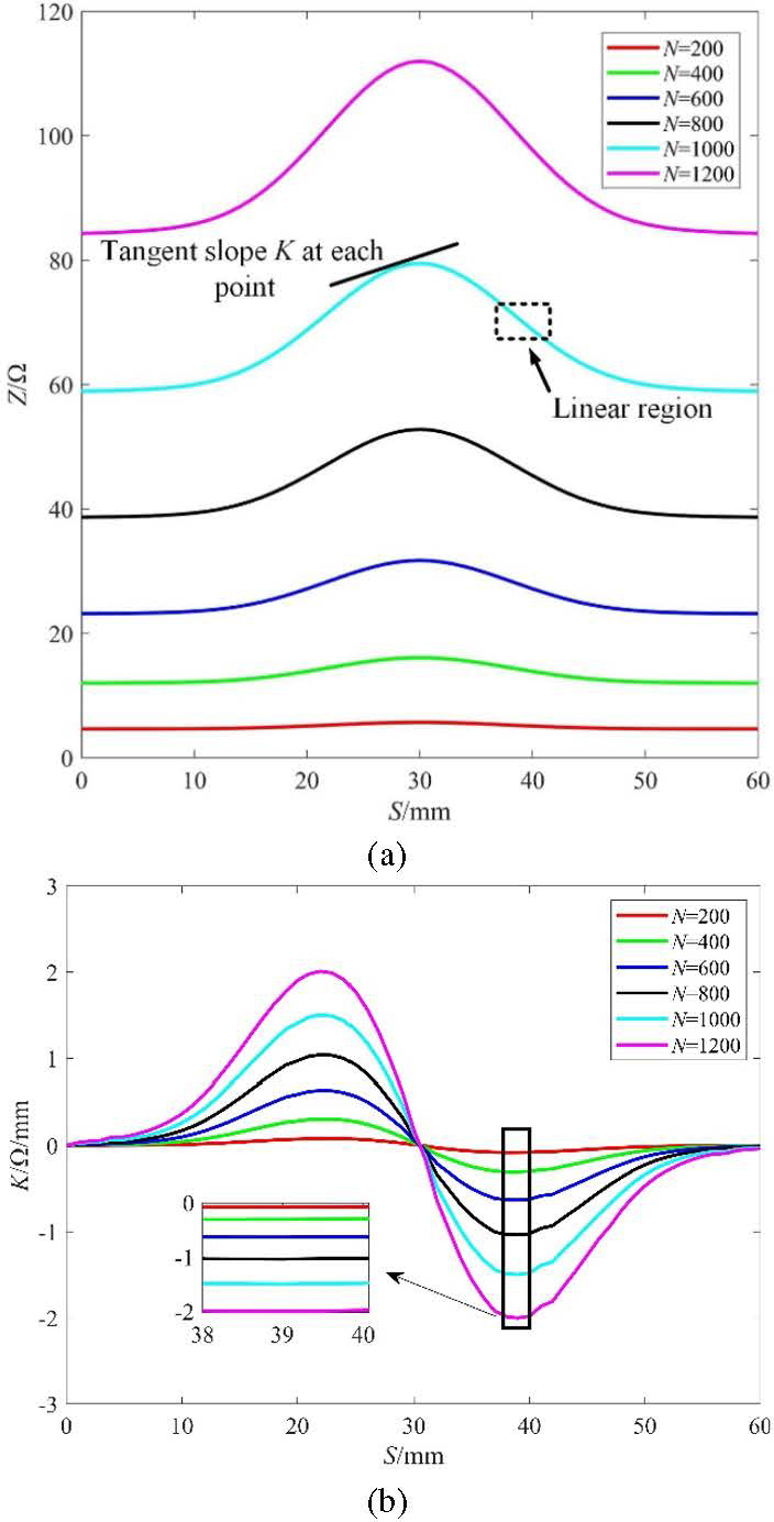
Figure 3: Impedance simulation results of different sensing coil turns N: (a) Z-S diagram for different turns N and (b) K-S diagram for different turns N.

A. Number of turns of sensing coil N

Based on the above simulation model and parameters, the number of turns of the sensing coil N is parametrically swept, the sweeping range is 200 $\sim$ 1200, the sweeping interval is 200, and the law of coil impedance value Z changing with the change of S is obtained. The simulation results are shown in Figs. 3 (a) and (b).

In Figs. 3 (a) and (b), the horizontal coordinate is the position S of the FB. The vertical coordinate of Fig. 3 (a) is the impedance value Z. The vertical coordinate of Fig. 3 (b) is the slope K of the tangent line at each point of the Z-S curve, that is, the change rate of Z with S. It can be observed from Figs. 3 (a) and (b) that there is a stable and regular correspondence between the position of the FB and the impedance of the sensing coil. There is a part of the Z-S curve where the changes in coil impedance and position represent an approximately linear change pattern, which is called the linear zone. Moreover, the slope of Z-S diagram in the linear region is the largest, that is, the change rate of the impedance value of the sensing coil is the largest. It can be observed from Fig. 3 (b) that in the process of decreasing the relative distance between the FB and the sensing coil, the change rate of the impedance value increases first. In the linear region, the change rate of the impedance value is basically unchanged, and then the change rate of the impedance value begins to decrease.

As the number of turns of coil N increases from 200 to 1200, the impedance value Z of the coil increases, the change of impedance value Z increases, and the slope of the linear region increases. Because the subsequent liquid viscosity measurement process needs to use a circuit to detect the coil impedance, in order to facilitate the circuit design, it is appropriate to use the impedance value of 50 $\sim$ 100 $Ω$ , and too many turns of the coil will lead to an increase in the volume of the coil, so the number of turns N $=$ 1000 is preferred.

B. Wire diameter d

Based on the simulation model and parameters mentioned above, the sensing coil’s turns N $=$ 1000 is set, and the wire diameter d is parametrically swept. The sweeping parameters are 0.1, 0.25, 0.5 and 1 mm, and the simulation results are obtained as shown inFig. 4.

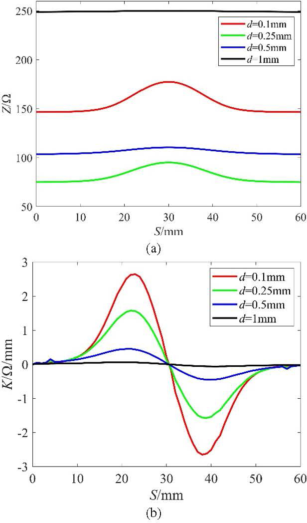
Figure 4: Simulation results of sensing coil impedance with different wire diameters d: (a) Z-S diagram of different wire diameters d and (b) K-S diagram of different wire diameters d.

It can be observed from Fig. 4 (a) that the impedance value of the sensing coil is the largest when d $=$ 1 mm, followed by the impedance value of d $=$ 0.1 mm. This is because the coil resistance value of d $=$ 0.1 mm is much larger than the resistance value of other wire diameter coils, and the coil reactance value of d $=$ 1 mm is much larger than the reactance value of other wire diameter coils, resulting in the coil impedance value of these two wire diameters being larger. It can be observed from Fig. 4 (b) that the impedance value of the sensor coil with d $=$ 0.1 mm and d $=$ 0.25 mm has a larger change rate. The smaller the wire diameter, the easier the wire is to break, increasing the difficulty of assembly. Moreover, the smaller the wire diameter, the higher the heat generated in the driving part, the greater the temperature change, and the greater the influence on the viscosity measurement results. Therefore, the wire diameter is optimized to d $=$ 0.25 mm.

C. Dimensions of the FB

The FB height h $_{1}$ should not be too large, because the higher the FB, the greater the electromagnetic force required to reset the FB and the longer the closed chamber. The height of the FB should not exceed 1/4 of the overall size of the device. The sensing coil’s wire diameter is set to 0.25 mm, and the FB height h $_{1}$ is parametrically swept. The sweeping range of h $_{1}$ is 12-20 mm, and the sweeping interval is 2 mm. The simulation results are shown in Fig. 5.

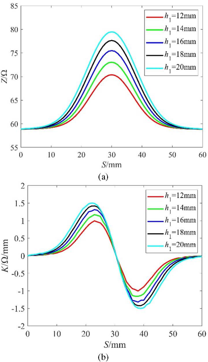
Figure 5: (a) Z-S diagrams of different FB heights h $_{1}$ and(b) K-S diagrams of different FB heights h $_{1}$ .

It can be observed from Figs. 5 (a) and (b) that as the height of the FB increases, the change of the impedance value of the sensing coil increases, and the length of the linear region also increases, which is conducive to the measurement of the FB velocity. The height of the FB is preferably set to h $_{1}$ $=$ 20 mm.

According to experience, the closer the FB’s radius r $_{1}$ is to the radius r $_{2}$ of the stainless steel tube, the smaller the stable velocity of the FB, and the longer the measurement time. Therefore, it is necessary to design falling bodies with different radii according to liquids with different viscosity ranges to ensure that the measurement time is adequate. The design is as follows: for liquid of 1-20 mPa $\cdot$ s, the FB radius r $_{1}$ is 3.9 mm; for liquid of 20-50 mPa $\cdot$ s, the FB radius r $_{1}$ is 3.85 mm; for liquid of 50-100 mPa $\cdot$ s, the FB radius r $_{1}$ is 3.8 mm.

IV. DRIVING SCHEME DESIGN

A. Upper and lower limit design

Through the simulation mentioned above, the dimensions of the FB and sensing coil are determined. Considering the ease of manufacturing and the aesthetics of the device, the drive coil and the sensing coil are of the same size. A 2D rotational axisymmetric model is constructed, as shown in Fig. 2 (a), to carry out a simulation study on the electromagnetic force of a FB generated by the driving coil. Set falling radius r $_{1}$ $=$ 3.8 mm and height h $_{1}$ $=$ 20 mm. Set coil width WH $=$ 16 mm, number of turns N $=$ 1000, wire diameter d $=$ 0.25 mm, and coil spacing D $_{2}$ $=$ 18 mm. Other simulation parameters are the same as those set in section III. Steady state study is carried out, current source is used to excite the driving coil, and the current value is set at 1 A. The parametric sweeping of position S of the FB is carried out, and the law of change of the electromagnetic force F with change of S is obtained. Voltage source is used to excite the sensing coil and the excitation voltage is set at 5 V. Frequency domain study is added and the frequency is set at 500 Hz. The parametric sweeping of the position S of the FB is carried out, and the law of coil impedance changing with change of S is obtained. The simulation results are shown in Fig. 6.

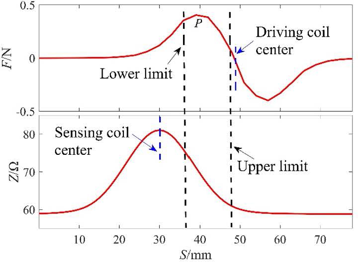
Figure 6: Upper and lower limits.

It can be observed from Fig. 6 that the electromagnetic force received by the FB in the process of approaching the driving coil increases first and then decreases, and there is a maximum force position P. When the FB is far away from the driving coil or close to the center of the driving coil, the electromagnetic force FB received is 0. Therefore, it is most appropriate to set the moving range of the FB to cover point P. When the FB approaches the center of the sensor coil, the impedance value increases. The impedance change rate increases first and then decreases, and reaches maximum value in the linear region. When liquid viscosity is measured, the process of falling is monitored by measuring the change of the impedance value of the sensing coil, and the time difference of the FB passing through the upper and lower limits is obtained. The moment when the FB begins to fall at the upper limit is the moment when the driving coil is powered off, and the moment when the FB reaches the lower limit is the moment when the coil impedance value no longer changes. Therefore, it is most appropriate to set the lower limit in the linear region with the largest impedance change rate. The movement range of the FB is set as l $_{t}$ $=$ 9 mm, and the position of the upper and lower limits is shown in Fig. 6.

B. Plug material

A 2D rotation axis symmetric model is constructed as shown in Fig. 7 (a). Set the FB radius r $_{1}$ $=$ 3.8 mm and height h $_{1}$ $=$ 20 mm. The width of the driving coil and the sensing coil is set WH $=$ 16 mm, the number of turns N $=$ 1000, and the wire diameter d $=$ 0.25 mm. Other simulation parameters are the same as the simulation parameter settings in section III. Current source is used to excite the driving coil, and the excitation current is 1 A. The mesh is set to “Physical Field Controlled Grid” and the unit size is selected as “Super Fine”. The plug material is set to iron and stainless steel, respectively, and a steady-state study is added. For iron, the relative magnetic permeability is set to 300. For stainless steel, the relative magnetic permeability is set to 1.2. The FB position S $_{1}$ is parametrically swept with a sweeping range of 0-9 mm. The law of the change of the electromagnetic force F with the change of S $_{1}$ is obtained. The simulation results are shown in Figs. 7 (b-d).

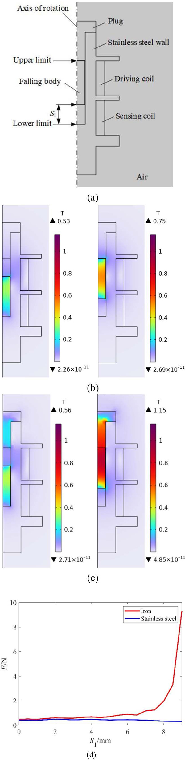
Figure 7: Electromagnetic simulation results of plug material: (a) diagrammatic figure, (b) magnetic flux density distributions of stainless steel plug, (c) magnetic flux density distributions of iron plug, and (d) comparison diagram of electromagnetic forces of different plug materials.

Figures 7 (b) and (c) show the distribution of magnetic field generated by the driving coil when plugs of different materials are at different positions. It can be seen from Figs. 7 (b) and (c) that, whether it is an iron plug or a stainless steel plug, the closer the distance between the FB and the driving coil, the stronger the magnetic field intensity around the FB. When the FB is far away from the driving coil, and the bottom surface of the FB is at the lower limit, whether it is an iron plug or a stainless steel plug, the maximum magnetic field intensity near the FB is about 0.3 T and, near the plug, the magnetic field intensity of the iron plug is much higher than that of the stainless steel plug. When the FB is close to the driving coil, and the top surface of the FB is at the upper limit, the magnetic field intensity near the FB and the plug is significantly higher for the iron plug than for the stainless steel plug.

Figure 7 (d) shows the electromagnetic force exerted on plugs of different materials at different positions. It can be observed from Fig. 7 (d) that when the FB is far away from the driving coil, and the bottom surface of the FB is close to the lower limit, whether an iron plug or a stainless steel plug is used, the electromagnetic force generated by the driving coil on the FB is similar, and the iron plug is slightly higher. When the FB is close to the driving coil, and the top surface of the FB is close to the upper limit, the electromagnetic force generated by the driving coil on the FB using an iron plug is significantly higher than that using a stainless steel plug, which is consistent with the conclusion obtained about the magnetic field strength in Figs. 7 (b) and (c). Therefore, iron is selected as the material of the plug.

V. EXPERIMENTS

A. Electromagnetic sensing and driving function verification

The liquid viscosity measuring device is designed and manufactured according to the parameters determined by the above simulations. The inner diameter r $_{2}$ of the stainless steel tube is 4.05 mm and the wall thickness is 5 mm. The number of turns of the driving coil and the sensing coil is N $=$ 1000, the width WH $=$ 16 mm, and the wire diameter d $=$ 0.25 mm. The center distance between the sensing coil and the driving coil is D $_{2}$ $=$ 18 mm. The thermocouple model used is GG-K-30-SLE, with an accuracy of 1.1 $^{\circ}$ C. In order to obtain a more accurate temperature, a higher precision thermocouple, such as the PT100, can be used. The distance between the thermocouple and the liquid is 10.45 mm. This distance can be changed by changing the depth distance of the thermocouple. The cross-sectional view of the device is shown in Fig. 8. An image of the device is shown in Fig. 9.

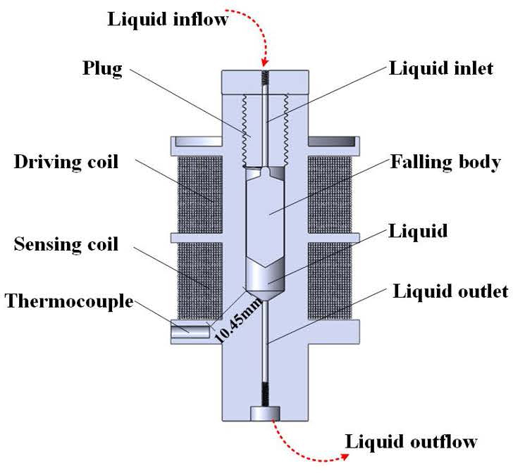
Figure 8: Cross-sectional view of the device.

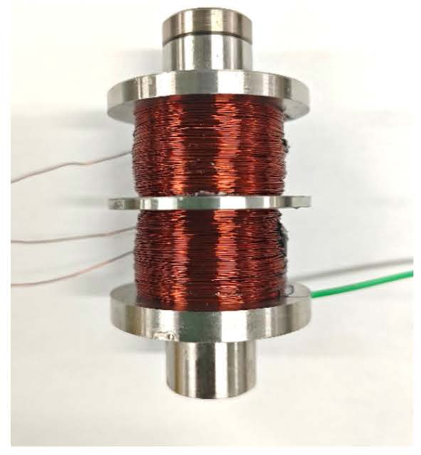
Figure 9: Image of the device.

The top of the FB is designed as an arc surface to prevent the possibility that the top of the FB cannot freely fall due to a large viscous force after resetting. The bottom of the FB is designed as a conical surface, which is matched with the bottom of the stainless steel chamber to ensure that the movement of the FB in the chamber is coaxial during each measurement. The height of the FB h $_{1}$ is 20 mm. The size of the FB is as follows: for liquids with viscosities 1-20 mPa $\cdot$ s, the radius of the FB r $_{1}$ is 3.93 mm; for liquids with viscosities 20-50 mPa $\cdot$ s, the radius of the FB r $_{1}$ is 3.88 mm; for liquids with viscosities 50-100 mPa $\cdot$ s, the radius of the FB r $_{1}$ is 3.79 mm; for liquids with viscosities 100-1265 mPa $\cdot$ s, the radius of the FB r $_{1}$ is 3.72 mm. The FB model diagram is shown in Fig. 10.

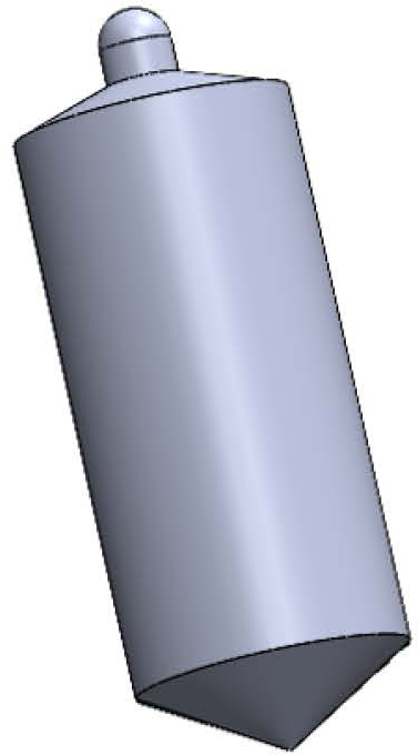
Figure 10: FB model diagram.

The measuring system is shown in Fig. 11, which includes the measuring device, the thermocouple, the measurement circuits, and the computer software.The microcomputer in the measurement circuits outputs a DC signal via internal DAC. This DC signal is amplified by a power amplifier and reaches the drive coil to generate a magnetic field. The iron plug and the coil form an electromagnet which generates electromagnetic force to reset the FB. The impedance detection circuit outputs the impedance value Z of the sensing coil in real time, which is collected by the microcontroller through the ADC to detect the position of the FB. The microcontroller sends the collected impedance data to the computer software for further analysis and calculation. A thermocouple is used to measure the liquid temperature and display it.

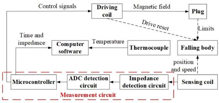
Figure 11: System block diagram.

In this experiment, dimethyl silicone oils with different viscosities are mixed in different proportions to provide 10 kinds of dimethyl silicone oils with different viscosities as test liquids covering the viscosity range of 9.5-1265 mPa $\cdot$ s. The viscosity of each test liquid is measured by the standard viscometer SV-10. Liquid #1 and liquid #2 are taken as experimental samples for showing falling impedance curves and are respectively loaded into the device for viscosity measurement. The radius of the FB used is r $_{1}$ $=$ 3.93 mm. In the experiment, the timing is started when the driving coil is powered off, and the impedance value of the sensing coil is recorded at each moment. The impedance value data and time data are plotted, and the results are shown in Fig. 12.

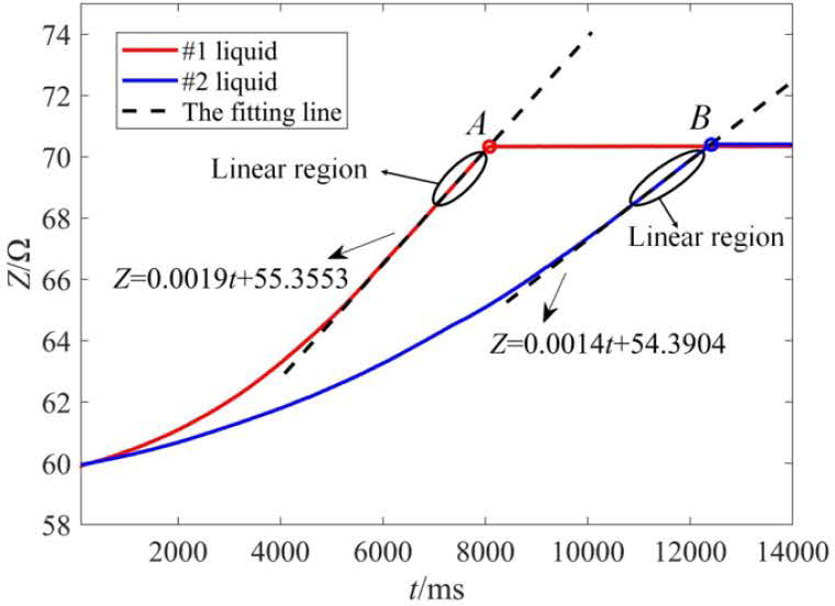
Figure 12: Tested impedance change curves of the sensing coil during the falling process of the FB when two liquids are respectively loaded for viscosity measurement.

It can be observed from Fig. 13 that when the FB falls in two different liquids, the impedance value Z no longer changes at points A and B, indicating that the FB has reached the lower limit at these two moments. In the Z-t curve, when verifying whether the linear region exists, starting from point A and point B, the program extracts data of 1/10 of the total falling time of the FB for verification of the linear zone. The program performs a linear fit on the data in the linear region. The linear region fitting results in Fig. 12 are as follows: Z $=$ 0.0019t $+$ 55.3553, R $^{2}$ $=$ 1 and Z $=$ 0.0013t $+$ 54.3903, R $^{2}$ $=$ 0.9998. The linearity is very good. The correctness of the detecting scheme of the FB position through the sensing coil is verified.

Figure 13: Experimental verification results of the FB reset scheme.

Figure 13 shows the curves of the impedance of the sensing coil changing with time after the driving coil is energized when the FB is in two different liquids. It can be observed from Fig. 13 that when the FB is in two different liquids, the driving coil generates electromagnetic force after the current is passed through the driving coil. The FB moves upward under the action of electromagnetic force, liquid viscous force, gravity and buoyancy, and the impedance value Z decreases. The impedance value Z of the sensing coil no longer changes at points C and D, indicating that the FB has been reset to the upper limit at these two moments. The feasibility of the scheme of resetting the FB through the electromagnetic force of an energized coil is experimentally verified.

B. Viscosity measurement results

To obtain the reference viscosity of different liquids, the SV-10 viscometer was used as a reference. The SV-10 viscometer has a measurement accuracy of $\pm$ 3% and a repeatability of 1% in the viscosity range 1-1000 mPa $\cdot$ s. First, the SV-10 sine wave vibration viscometer was used to measure the viscosity of 10 test liquids at different temperatures, and a linear function was used to fit the temperature and viscosity data. The viscosity-temperature curves of these 10 test liquids in the temperature range 20-35 $^{\circ}$ C were obtained. Then, the 10 blends of dimethyl silicone oils were divided into four groups according to their viscosity, corresponding to the FBs in the four measuring ranges. Four types of FBs needed to be calibrated separately. Taking the first group as an example, the #2 liquid was put into the experimental device, and the falling time t of the FB was recorded. At the same time, the temperature of the liquid at this time was recorded, and the viscosity $η$ of the liquid at this time through the viscosity-temperature curve of #2 liquid is obtained. Since the temperature does not change much, it is believed that the density of dimethyl silicone oil only changes slightly, and 1- $ρ_{l i q} / ρ_{s}$ is a determined calculated value of 0.8718. The calibration coefficient A is calculated according to equation (2). An image of the SV-10 viscometer is shown in Fig. 14, and the fitting results are shown in Fig. 15. The grouping and resulting instrument coefficients A are shown in Table 1.

Figure 14: SV-10 sine wave vibration viscometer.

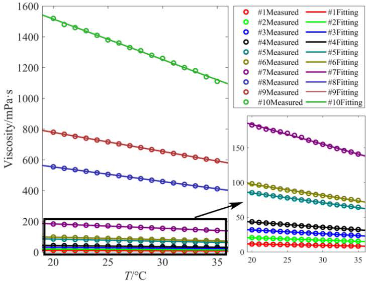
Figure 15: Viscosity measurements and results of different initial viscosities at different temperatures.

Table 1: Instrument coefficients

Number	1- $ρ_{l i q} / ρ_{s}$	*r $_{1}$ /mm*	*A/mPa*
#1	0.8718	3.93	1.5293195
#2
#3		3.88	4.1635895
#4
#5		3.79	16.399665
#6
#7		3.72	40.345561
#8
#9
#10

Table 2: Viscosity measurement results

Liquid Number	*T/ ${}^{\circ}C$*	$η_{r}$ /mPa $\cdot$ s	*t/s*	$η_{m}$ /mPa $\cdot$ s	Relative Error
#1	30.3	9.52	7.11	9.483	-0.4%
#2	29.5	17.29	12.56	16.74	-3.2%
#3	30.3	26.14	7.44	27.00	-3.3%
#4	30.2	35.58	9.64	34.99	1.6%
#5	30.1	70.81	4.76	68.07	-3.8%
#6	30.1	81.42	5.54	79.16	2.7%
#7	32.1	149.3	4.44	156.17	4.3%
#8	31.8	442.2	12.81	450.57	1.9%
#9	30.1	653.4	18.72	658.44	0.8%
#10	29.5	1265	36.56	1285.93	1.6%

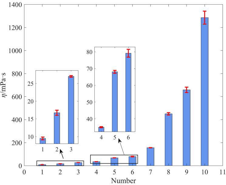
Figure 16: Error bar plot of the test results.

Using the manufactured FB viscosity measuring device, the viscosity of 10 liquids was measured. The liquid temperature during measurement was obtained through the thermocouple, and the viscosity value of the liquid to be measured at the temperature was obtained according to the viscosity-temperature fitting curve as the reference viscosity value $η_{r}$ . The time t of the FB falling in liquids of different viscosities is measured through the sensing coil, and the measured value $η_{m}$ of the liquid viscosity is calculated according to equation (2). The movement range of the FB is only 9 mm, which can make the closed cavity in the stainless steel tube very small. Only 1 mL of liquid is needed to completely fill the closed cavity containing the FB. The falling time of the FB is between 4 and 37 seconds. The falling time of the FB in each liquid was measured three times and the average value was calculated. The viscosity was calculated using the FB method formula and recorded in Table 2. According to Table 2, it can be calculated that the average absolute value of the relative error is 0.22%, and the maximum value is 4.3%. In order to visually display the error results, the error bar plots for the 10 test liquids are shown in Fig. 16. It can be observed in Fig. 16 that the error bar length is short, which verifies the accuracy of the device.

VI. HIGH-TEMPERATURE AND HIGH-PRESSURE TOLERABILITY ANALYSIS

A. Theoretical analysis of high-temperature tolerability

Our measuring system consists of 304 stainless steel cylinders, two enameled wire electromagnetic coils, an iron plug, an iron FB and measuring circuit. The stainless steel cylinder, iron plug and iron FB are in direct contact with the high-temperature and high-pressure liquid to be measured. Two electromagnetic coils are placed near the high-temperature and high-pressure liquid. The measuring circuit is at a distance from the high-temperature and high-pressure liquid. For general industrial applications, 304 stainless steel is generally safe to use in the temperature range up to 800 $^{\circ}$ C. The Curie temperature of iron is 770 $^{\circ}$ C. Within this temperature range, iron can maintain strong magnetism. The temperature resistance of enameled wire electromagnetic coils mainly depends on the type of insulating paint used. The temperature resistance grade of ordinary polyester enameled wire is 130 $^{\circ}$ C. The temperature resistance grade of modified polyester enameled wire is 155 $^{\circ}$ C. The temperature resistance grade of polyimide enameled wire is 240 $^{\circ}$ C. The enameled wire we use can tolerate high temperatures of 130 $^{\circ}$ C. Therefore, the working temperature range of this device can reach 130 $^{\circ}$ C.

B. Simulation analysis of high-pressure environment tolerability

Simulation verification of pressure resistance capability of the developed closed chamber device for measuring liquid viscosity was carried out with COMSOL software. A 2D rotational axial symmetry model is constructed, as shown in Fig. 17 (a). Model dimensions are the same as those in section IV, part B. The closed cavity material is stainless steel whose density is 7850 kg/m $^{3}$ , Young’s modulus is 200 GPa, and Poisson’s ratio is 0.3. Solid mechanics was chosen as the physics field. The model is set to linear elastic material. Wherein, the density, Young’s modulus and Poisson’s ratio are all determined by “from material” option. The outer boundary of the model is set to “free”, and boundary loads are added to the inner boundary of the model. The load diagram is shown in Fig. 17 (b). The pressure is the parameter to be swept, the bottom boundary of the model is set as a fixed constraint, and the “rigid body motion suppression” condition is added to the entire model. The mesh is set to “Physics Control Mesh” and the unit size is selected to “Ultra-Fine”. A steady state study is added, the pressure sweeping range is 10 $\sim$ 100 MPa, and the sweeping interval is 10 MPa. The sweeping simulation results of the deformation and stress distribution of the device under different loads are obtained, as shown in Figs. 17 (c) and (d). The inner boundary stress distribution results are shown inFig. 17 (e).

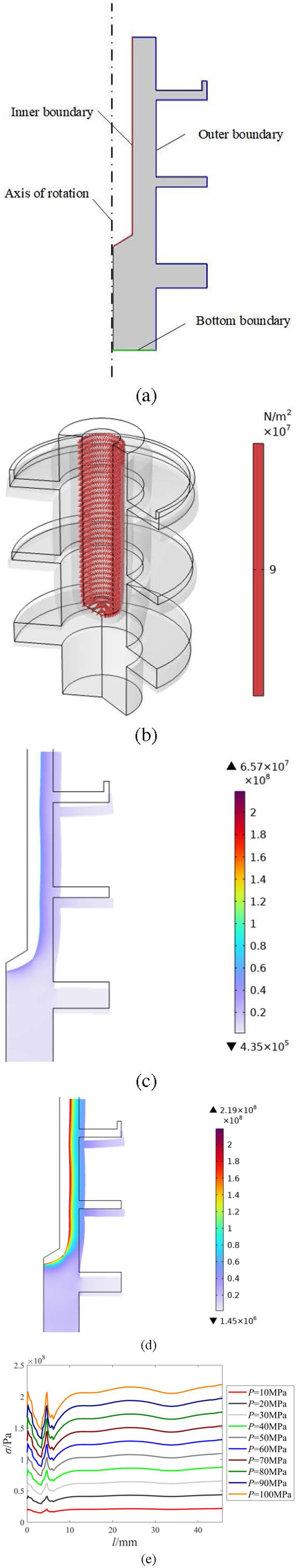
Figure 17: Closed cavity pressure simulation: (a) simulation model, (b) boundary load diagram, (c) device deformation and stress distribution under 30 MPa load, (d) device deformation and stress distribution under 100 MPa load, and (e) internal surface stress distribution.

It can be observed from Figs. 17 (c) and (d) that as the boundary load increases, the stress of the sealed cavity device increases. Under a load of 30 MPa, the maximum stress of the device is 65.7 MPa. Under a load of 100 MPa, the maximum stress of the device is 219 MPa. It can be observed from Fig. 17 (e) that there is a large stress concentration at the intersection of the inner boundary cylindrical surface and the conical surface (at l $=$ 5 mm). On the cylindrical surface, the stress distribution is relatively uniform, and the stress on the cylinder surface is roughly the same as the stress at the intersection. When the boundary load increases to 100 MPa, the stress on the device may be greater than the allowable stress of the adopted 304 stainless steel, whose yield strength is 205 $\sim$ 215 MPa. Therefore, the device can tolerate liquid pressure of 100 MPa.

VII. CONCLUSION

This paper proposes a FB-based device for measuring liquid viscosity in a closed cavity with simple structure, small size, small amount of sample required, and fast FB reset speed. It includes a stainless steel closed tube with an iron FB, an iron plug, one driving coil, and one sensing coil. Through electromagnetic finite element simulation, the characterization ability of a single sensing coil impedance on the position of a FB and its influencing factors are studied, and the ability of a single driving coil to attract and reset a FB and its enhancement factors are studied. Dimethyl silicone oil viscosity measurement experiments are carried out to prove the feasibility of the designed device. The following conclusions can be obtained.

(1) There is a stable correspondence between the position of the FB and the impedance of the sensing coil; there is a region where the coil impedance and position show an approximately linear change pattern. Via elaborative size design, the lower limit of the FB’s motion is set in this linear zone, so that the moment when the FB reaches the lower limit point can be accurately determined, and then the time difference method can be used to conveniently and accurately measure the steady speed of the FB.

(2) As the number of turns of the sensing coil increases and the wire diameter decreases, the coil impedance value and its variation increase, which is beneficial to determining the moment when the FB reaches the upper and lower limit positions. As the height of the FB increases, the change in the impedance of the sensing coil increases, and the length of the linear zone also increases, which is beneficial to the detection of the moment when the FB moves to the lower limit point.

(3) The electromagnetic force received by the FB when approaching the driving coil first increases and then decreases, and there is a maximum force position. Designing the movement range of the FB to make this range cover this point and setting the plug material to iron can make the FB gain greater electromagnetic attraction force and ensure its successful reset.

(4) Based on the simulation results, a FB viscosity measuring device is produced. Experiments have verified that a single driving coil can reliably reset the FB, and a single sensing coil can measure the position of the FB and characterize the liquid viscosity. The size of the closed cavity is very small, and the moving distance of the FB is only 9 mm. For dimethyl silicone oil with a viscosity range of 9.5-1265 mPa $\cdot$ s, only 1 mL of liquid sample is needed to measure the viscosity. The average absolute value of the relative measurement error is 0.22%, and the maximum value is 4.3%.

ACKNOWLEDGEMENT

This work was supported in part by National Natural Science Foundations of China under Grant No. 62073233.

REFERENCES

[1] H. L. Wang, Z. Li, and J. W. Zhao, “Discussion of viscosity measurement of liquids,” Physical Experiment of College, vol. 7, no. 2, pp. 33-35, June 1994.

[2] B.-H. Shi, S. Chai, L.-Y. Wang, X. Lv, H.-S. Liu, H.-H. Wu, W. Wan, D. Yu, and J. Gong, “Viscosity investigation of natural gas hydrate slurries with anti-agglomerants additives,” Fuel, vol. 185, pp. 323-338, Dec. 2016.

[3] S. Gautam, C. Guria, and L. Gope, “Prediction of high-pressure/high-temperature rheological properties of drilling fluids from the viscosity data measured on a coaxial cylinder viscometer,” SPE Journal, vol. 26, no. 05, pp. 2527-2548, Oct. 2021.

[4] Y. F. Guo, “Research on the current situation and high-quality development path of coal-to-liquid: research on the high-quality development of coal direct liquefaction technology,” Inner Mongolia Petrochemical Industry, vol. 47, no. 9, pp. 4-8, Sep. 2021.

[5] R. Wiśniewski, R. M. Siegoczyński, and A. J. Rostocki, “Viscosity measurements of some castor oil based mixtures under high-pressure conditions,” High Pressure Research, vol. 25, no. 1, pp. 63-68, Mar. 2005.

[6] A. Miyara, Md. J. Alam, K. Yamaguchi, and K. Kariya, “Development and validation of tandem capillary tubes method to measure viscosity of fluids,” Transactions of the Japan Society of Refrigerating and Air Conditioning Engineers, vol. 36, no. 1, pp. 18-47, Mar. 2019.

[7] M. E. Kandil, K. N. Marsh, and A. R. H. Goodwin, “Vibrating wire viscometer with wire diameters of (0.05 and 0.15) mm: Results for methylbenzene and two fluids with nominal viscosities at T $=$ 298 K and p $=$ 0.01 MPa of (14 and 232) mPa $\cdot$ s at Temperatures between (298 and 373) K and Pressures below 40 MPa,” Journal of Chemical Engineering Data, vol. 50, no. 2, pp. 647-655, Mar. 2005.

[8] J. B. Zhang, X. Y. Meng, G. S. Qiu, and J. Wu, “Development of vibrating-wire viscometer for liquid at high pressure,” Journal of Xi’an Jiaotong University, vol. 46, no. 11, pp. 30-34, Nov. 2012.

[9] M. Hosoda, Y. Yamakawa, and K. Sakai. “Electromagnetically spinning viscometer designed for measurement of low viscosity in low shear rate region,” Japanese Journal of Applied Physics, vol. 63, no. 4, Mar. 2024.

[10] X. W. Zhang and P. He, “A high-temperature and high-pressure oil-coal slurry viscosity determination device,” CN. Patent 200952994, 26 Sep. 2007.

[11] P. W. Bridgman, “The viscosity of liquids under pressure,” Proceedings of the National Academy of Sciences, vol. 11, no. 10, pp. 603-606,1925.

[12] P. W. Bridgman, “The effect of pressure on the viscosity of forty-three pure liquids,” Proceedings of the American Academy of Arts and Sciences, vol. 61, no. 3, p. 57, 1926.

[13] J. Lohrenz, G. W. Swift, and F. Kurata, “An experimentally verified theoretical study of the falling cylinder viscometer,” AIChE Journal, vol. 6, no. 4, pp. 547-550, 1960.

[14] E. Ashare, R. B. Bird, and J. A. Lescarboura, “Falling cylinder viscometer for non-Newtonian fluids,” AIChE Journal, vol. 11, no. 5, pp. 910-916, 1965.

[15] N. D. Cristescu, B. P. Conrad, and R. Tran-Son-Tay, “A closed form solution for falling cylinder viscometers,” International Journal of Engineering Science, vol. 40, no. 6, pp. 605-620, Mar. 2002.

[16] F. Gui and T. F. Irvine, “Theoretical and experimental study of the falling cylinder viscometer,” International Journal of Heat and Mass Transfer, vol. 37, pp. 41-50, Mar. 1994.

[17] J. B. Irving and A. J. Barlow, “An automatic high pressure viscometer,” Journal of Physics E: Scientific Instruments, vol. 4, no. 3, pp. 232-236, Mar. 1971.

[18] V. Průša, S. Srinivasan, and K. R. Rajagopal, “Role of pressure dependent viscosity in measurements with falling cylinder viscometer,” International Journal of Non-Linear Mechanics, vol. 47, no. 7, pp. 743-750, Sep. 2012.

[19] S. Bair, “A routine high-pressure viscometer for accurate measurements to 1 GPa,” Tribology Transactions, vol. 47, no. 3, pp. 356-360, July 2004.

[20] S. Bair, “A new high-pressure viscometer for oil/refrigerant solutions and preliminary results,” Tribology Transactions, vol. 60, no. 3, pp. 392-398, May 2017.

[21] K. R. Harris, “A falling body high-pressure viscometer,” International Journal of Thermophysics, vol. 44, no. 12, p. 184, Dec. 2023.

[22] S. Yang, K. Hirata, T. Ota, Y. Mitsutake, and Y. Kawase, “Impedance characteristics analysis of the non-contact magnetic type position sensor,” Electronics and Communications in Japan, vol. 94, no. 3, pp. 33-40, Mar. 2011.

[23] S.-H. Yang, K. Hirata, T. Ota, and Y. Kawase, “Impedance linearity of contactless magnetic-type position sensor,” IEEE Transactions on Magnetics, vol. 53, no. 6, pp. 1-4, June 2017.

[24] X. Wang, S. Zhu, and X. Wang, “Experimental system for high-pressure viscosity measurement based on the falling-body method,” Journal of Engineering Thermophysics, 2020.

[25] C. J. Schaschke, S. Allio, and E. Holmberg, “Viscosity measurement of vegetable oil at high pressure,” Food and Bioproducts Processing, vol. 84, no. 3, pp. 173-178, Sep. 2006.

[26] C. J. Schaschke, S. Abid, I. Fletcher, and M. J. Heslop, “Evaluation of a falling sinker-type viscometer at high pressure using edible oil,” Journal of Food Engineering, vol. 87, no. 1, pp. 51-58, July2008.

BIOGRAPHIES

Kun Zhang received her master’s degree in analytical chemistry from Jilin University (Changchun) in 2008. She is currently working at Shandong Non-Metal Materials Research Institute. Her research interests mainly involve chemical measurement and viscosity and density detection technology.

Hongbin Zhang (corresponding author) received the B.Sc. degree in measurement and control technology and instrument from Hebei University of Technology, Tianjin, China, in 2022. He is currently pursuing the M.Sc. degree in Tianjin University, under the guidance of Associate Professor Xinjing Huang. His research interests include pipeline stress measurement, signal feature extraction, and the application of magnetic sensors.

Yuan Xue has his bachelor’s degree, and works as an engineer, first-class registered metrology, national laboratory qualification accreditation assessor, metrology standard evaluator. He entered the China Institute of Testing Technology in 2004, and since then he has been mainly engaged in metrology and testing technology research and reference material research.

Jinyu Ma received her B.E. and M.E. degrees in Instrument Science and Technology from Shandong University of Science and Technology, Qingdao, China, in 2010 and 2012, respectively. She received her Ph.D. degree in Instrument Science and Technology from Tianjin University, Tianjin, China, in 2016. In 2016, she joined the Sensor and Electronic Testing Laboratory of Tianjin University as a lecturer and engineer. She also works at State Key Laboratory of Precision Measurement Technology and Instrument, Tianjin University. Her research topics mainly cover electric sensing and measurement, precision measuring circuit, measurement and control based on embedded system.

Jiqing Han received his master’s degree in chemical engineering from Qingdao University in 2015. Currently, he works at Shandong Nonmetallic Materials Research Institute as an associate researcher. His research interests are mainly in oil property measurement.

Xinjing Huang (corresponding author) received the B.E. and Ph.D. degrees in instrument science and technology from Tianjin University, Tianjin, China, in 2010 and 2016, respectively. He is currently an Associate Professor with the School of Precision Instrument and Opto-Electronics Engineering, Tianjin University, where he also works with the State Key Laboratory of Precision Measurement Technology and Instruments. His research topics mainly cover acoustic and/or electromagnetic sensing and measurement technologies.