Design of Ultra-Wideband Antenna Based on Gaussian Process Regression and Genetic Algorithms

Da Li Mi¹, Xi Wang Dai^{1, 2}, Jun Shi Zhao¹, Ze Li¹, Gang Li³, and Hui Hong¹

¹Shaoxing Integrated Circuit Institute & School of Electronics and Information Hangzhou Dianzi University, Hangzhou, Zhejiang 310018, China
mi_dali@qq.com, xwdai@hdu.edu.cn, 1258042732@qq.com, 1223406727@qq.com, hongh@hdu.edu.cn

²State Key Laboratory of Millimeter Waves Southeast University, Nanjing 210096, China

³Hubei Key Laboratory of Low Dimensional Optoelectronic Materials and Devices Hubei University of Arts and Science, Xiangyang 441053, China
ligang_hbuas@vip.163.com

Submitted On: July 07, 2024; Accepted On: December 01, 2025

ABSTRACT

Gaussian Process Regression (GPR) algorithm and Genetic Algorithms (GA) are used to design a scheme suitable for antenna optimization in this paper. GPR algorithms are used to build so-called surrogate models, or machine learning models, to replace full-wave simulation calculations to save time. GA is used to find the optimal solution that satisfies the optimization objective. The optimal solution obtained by GA is re-calculated with full-wave electromagnetic simulation. The surrogate model can be updated with new data when the full-wave simulation results don’t meet the target. An ultra-wideband (UWB) antenna is designed by using this optimization scheme. Six structural parameters of the UWB antenna are used to optimize the design, and a total of 10 groups are used to train the surrogate model. Finally, the optimization is completed through 7 iterations. Finally, the UWB antenna is analyzed, fabricated and tested, which shows an operating frequency band of 2.95–11.43 GHz, and a physical size of 30 $\times$ 27 $\times$ 1.6 mm³.

Keywords: Gaussian Process Regression (GPR), Genetic Algorithms (GA), ultra-wideband (UWB) antenna.

1 INTRODUCTION

Ultra-wideband (UWB) technology is a practical and effective wireless communication technology, widely used in local area network, intelligent transportation, radio frequency identification and other fields, and has strong anti-interference performance, low transmission power spectrum density, high positioning accuracy and many other advantages. As a device for transmitting and receiving wireless signals, antennas have different types according to different application scenarios. The antenna coving 3.1–10.6 GHz can be suitable for UWB application according to the regulations of the United States Federal Communications Commission (FCC).

The common methods to realize UWB antenna include loading parasitic patch, impedance loading technology and slot technology. Among them, the parasitic patch and slot technology are used to form multiple resonant frequencies, and make the resonant frequencies close together, to achieve the purpose of broadening the bandwidth. However, there is no theoretical formula to describe the relationship between the size of the parasitic patch and the operating bandwidth of antennas. Designers usually calculate its performance parameters, such as the scattering parameters, through electromagnetic simulation software. Machine learning (ML) algorithms [1, 2, 3, 4] can make up for this shortcoming and build a so-called surrogate model between the two to describe this nonlinear relationship. This surrogate model of the antenna is known as the ML model. At present, ML algorithms used for antenna optimization include support vector machine (SVM) [5, 6, 7], deep neural network (DNN) [8, 9] and K-nearest neighbor (KNN) [10]. The Gaussian process is a new supervised learning algorithm that learns the input-output relationship of functions based on empirical data. In the 1990s, Poggio and Girosi first combined Gaussian processes with neural networks for research. The Gaussian Process Regression (GPR) algorithm is also widely used in antenna design [11, 12, 13]. Furthermore, these methods can obtain scattering parameters from specific physical models. However, physical dimensions cannot be obtained from the scattering parameters. First proposed by Professor J. Holland in 1975, Genetic Algorithm (GA) is a randomized search method that draws on the evolutionary laws of the biological world. The GA can quickly obtain the optimal solution of an equation or system of equations. In the antenna design, GA can obtain a specific antenna model that meets certain conditions [14, 15, 16, 17]. UWB and dual-band antennas are designed with GPR and GA in [18]. However, the surrogate model cannot be updated with new data, and the size of antenna is relatively large. With the concept of performance-driven modelling, the technologies of Kriging, radial basis functions, or polynomial chaos expansion are also recently proposed and developed for antenna design [19, 20, 21, 22].

In this paper, an optimization scheme is designed based on GPR and GA, and a UWB antenna is designed based on this optimization scheme. There is also a dual-band antenna as an additional example. Although the antenna optimization design can be completed by full-wave electromagnetic software such as HFSS and CST, the optimization efficiency is relatively low. Full-wave calculations are invoked when using GA for optimization in simulation software, which is the most time-consuming step. For the UWB structure proposed in this paper, a full-wave simulation takes 31.4 seconds at a time, while the surrogate model trained with GPR takes only 118 milliseconds. When iterations are ongoing, the time savings are considerable. Another advantage of using algorithms to complete optimization algorithms is that there is no need for the designer to think about the relationship between physical size parameters and antenna performance parameters. The GPR can establish a nonlinear relationship. The designed UWB antenna is obtained by 7 iterations. Its operating frequency band is 2.95–11.43 GHz and its physical size is 30 $\times$ 27 $\times$ 1.6 mm³.

2 ANTENNA STRUCTURE AND OPTIMIZATION SCHEME

The circuits of the designed UWB antenna are printed on the FR4 substrate with a dielectric constant of 4.4 and a loss tangent of 0.02, as shown in Fig. 1. The front patch (in red) is an irregular polygon. The back patch (in blue) is a polygon of a large rectangle dug out of a small rectangle. The aim of the algorithm proposed is to design an UWB antenna within a specified size range. The objective of the design is measured by the $| S_{11} |$ value less than $-$ 10 dB in the 3.1–10.6 GHz band range.

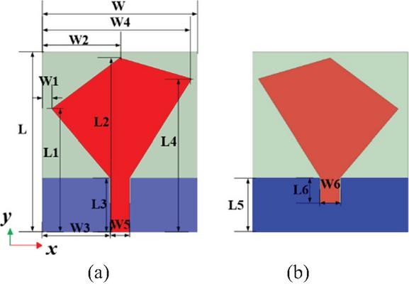
Figure 1 Geometry of proposed UWB antenna: (a) top view and (b) bottom view.

Table 1 Parameters of antenna (units: mm)

Parameter	L $_{1}$	W $_{1}$	L $_{2}$	W $_{2}$	L $_{3}$
Value	20.49	1.62	29	13.5	9
Parameter	W $_{3}$	L $_{4}$	W $_{4}$	L $_{5}$	W $_{5}$
Value	11.4	25.51	25.01	9	3.2
Parameter	L $_{6}$	W $_{6}$	L	W	/
Value	4.18	3.5	30	27	/

Figure 1 shows the structure after optimization. The specific size parameters are shown in Table 1. Since there is no theoretical formula to guide the optimal design for the physical size of the front and back patches and the scattering parameters of this antenna, the GPR algorithm is used to establish the surrogate model to describe this nonlinear relationship between the two. This surrogate model is also the GPR model. Further, the GA is used to find the physical size values that satisfy the optimization conditions. The overall flow chart of the designed optimization scheme is shown in Fig. 2, which can be divided into five steps.

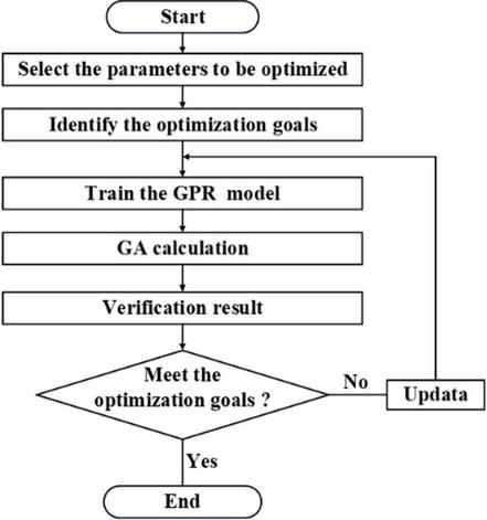
Figure 2 Flowchart of the optimization scheme.

Step 1: Analyze the characteristics of the antenna model and set the performance index. Through full-wave electromagnetic simulation software (such as HFSS and CST) scanning analysis of parameters, the physical size of the UWB antenna parameters $L_{1}$ , $W_{1}$ , $L_{4}$ , $W_{4}$ , $L_{6}$ , $W_{6}$ and frequency to a total of seven parameters as the input variables of the surrogate model, $| S_{11} |$ as the performance index (that is, the output variables of the surrogate model). The optimal solution obtained by the GA is the six structural parameters of this antenna. The reason for choosing these six parameters is that they have the greatest effect on the S-parameter of this antenna. As the target of the design is the UWB antenna, the $| S_{11} |$ value is required to be less than -10 dB in the frequency range of 3.1–10.6 GHz. Thus, that’s the optimization condition that needs to be met.

Step 2: Collect the initial dataset (sample set). First, the variable range of the input variable is determined. $L_{1}$ : 20–26 mm, $W_{1}$ : 0.5–3.5 mm, $L_{4}$ : 20–26 mm, $W_{4}$ : 23.5–26.5 mm, $L_{6}$ : 2–6 mm, $W_{6}$ : 3–6 mm. In the frequency range (2–12 GHz), 101 frequencies are selected at equal intervals (equidistant sampling), that is, the step value of frequency is 0.1 GHz. The initial dataset is the $| S_{11} |$ values of 10 groups of UWB antennas in this frequency range. Each set of data (101 frequencies) requires an HFSS simulation to collect. There are a total of 1010 data here. One HFSS simulation took 31.4 seconds, for a total of 314 seconds. The physical dimension parameter is evaluated by the Latin Hypercube Sampling (LHS), which is required to sample 10 times. The LHS is divided into three steps: stratification, sampling and out-of-order. The samples extracted by LHS are relatively uniform, which can avoid the phenomenon of data aggregation to some extent.

Step 3: Parameter selection of the GPR model (surrogate model). This step trains the GPR model in the dataset collected in the previous step. This model uses the coefficient of determination ( $R^{2}$ ) as the evaluation index. When its value is greater than 0.9, the GPR model can be used; otherwise, it needs to be retrained. The GPR model is also the surrogate model of the UWB antenna. The calculation formula of $R^{2}$ is:

R^{2} = 1 - \frac{\sum_{i = 1}^{n} {(y_{i} - \hat{y})}^{2}}{\sum_{i = 1}^{n} {(y_{i} - \bar{y})}^{2}},

(1)

where $y_{i}$ is the real observed values, $\bar{y}$ is the average value of real observed values, and $\hat{y}$ is the predicted value [23]. The larger $R^{2}$ , the more accurate the GPR model. The value of $R^{2}$ is between 0 and 1.

Step 4: Objective function setting and parameter selection of the GA. In this step, according to the design rules of the objective function of GA, the optimization objective of the antenna needs to be abstracted into the maximum or minimum value of a function (the so-called objective function). This optimization can be considered successful when the values of $f \in [3.1, 10.6]$ and $| S_{11} |$ is less than $-$ 10 dB. Let the objective function $U (L_{1}, W_{1}, L_{4}, W_{4}, L_{6}, W_{6}$ ) be the number of frequencies when $| S_{11} |$ is greater than $-$ 10 dB. When the minimum value of U is 0, the optimization is successful. It can be expressed by the formula:

Min {U (L_{1}, W_{1}, L_{4}, W_{4}, L_{6}, W_{6})} = 0 .

(2)

There are three important operations in GA, namely selection, crossover and mutation. The GA used in this paper is the differential evolution template. The coding method is real integer (RI) mixed coding, the population size is 50, the maximum number of generations is 50, and the crossover probability is 0.7.

Step 5: Validation and iterative optimization. After setting GA in the previous step, the iterative calculation can be carried out, and the obtained result is the physical size value of the UWB antenna (the optimal solution of the objective function).

It is worth mentioning that GA calculates the $| S_{11} |$ value through the GPR model trained in the third step instead of the full-wave electromagnetic calculation. This step not only obtains the optimal solution but also saves a lot of time. A surrogate model trained with GPR algorithm takes only 118 milliseconds. The optimal solution obtained by GA is re-calculated with full-wave electromagnetic simulation for verification. If the simulation value still completes the target, it indicates that the optimization is completed. If the simulation value does not reach the target, it needs to be re-optimized, that is, enter the iteration. Each iteration will add a new value to the initial dataset. This is the update to the dataset. Each iteration includes GPR model training, GA calculation and full-wave simulation verification. The time for one iteration is 41 seconds.

3 TEST RESULTS AND ANALYSIS

After only 7 iterations, the UWB antenna is obtained as shown in Fig. 1. The time for iterations is 287 seconds, which does not include the initial data sampling time. This is the optimized structure. The reference structure before optimization is shown in Fig. 4. The result after the completion of the first iteration is shown in Fig. 3. After the completion of each iteration, there are similar results and tips. Each iteration for proposed algorithm includes steps of GA calculation and electromagnetic (EM) simulation verification, shown in Fig. 2. EM simulation verification alone takes approximately 31.4 s. GA is a stochastic optimization algorithm. When the optimal solution of the objective function is obtained, the simulation speed of GA will be accelerated.

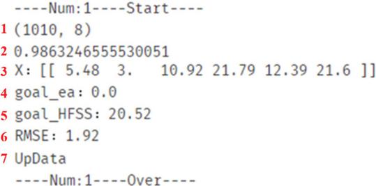
Figure 3 Result of the first iteration.

Line 1 represents the initial dataset structure, with 1010 samples. There are 10 full-wave simulation results. Each simulated result is sampled 101 data from 2 GHz to 12 GHz with a step of 0.1 GHz.

Line 2 indicates that the $R^{2}$ of the trained GPR model is 0.9863, indicating that the accuracy meets the requirements.

Line 3 shows the results given by the GA.

Line 4 indicates that when the GPR model is used for calculation, the value of the objective function is 0, which indicates that the GA has calculated the optimal solution.

Line 5 indicates that the objective function value obtained by the full-wave simulation software (HFSS) is 20, which does not meet the requirements. The number 20 indicates that 20 frequencies do not meet the requirement. The optimal solution is obtained by iterative calculation.

Line 6 indicates that the root-mean-square error (RMSE) between the full-wave simulation value and the GPR model calculation value is 1.92 under the dimension parameter value in Line 3.

Update in Line 7 indicates that the initial dataset has been updated. When the value of goal_HFSS in Line 5 is 0, it indicates that the optimization goal is completed and the iteration can be quit. If there is a second iteration, the sample number is updated to 1111.

The optimized antenna dimensions are $L_{1} = 20.49$ mm, $W_{1} = 1.62$ mm, $L_{4} = 25.51$ mm, $W_{4} = 25.01$ mm, $L_{6} = 4.18$ mm, $W_{6} = 3.50$ mm. This is also the optimal solution obtained by the GA. The patch structure of the original antenna is a parallelogram, that is, $L_{1} = L_{4} = 19$ mm, $W_{1} = 3.5$ mm, $W_{4} = 23.5$ mm, as shown in Fig. 4. Of course, as the optimization goal changes, the number of iterations and the optimal solution will also change. The final optimization results show that the optimization method using the algorithm can break through the traditional regular polygon structure.

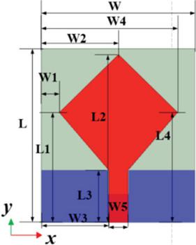
Figure 4 Geometry of the reference antenna.

Take this antenna as the reference and compare it with the optimized antenna’s $| S_{11} |$ curve, as shown in Fig. 5. It can be seen that the optimized scheme has achieved good results. Within the frequency band 3.1–10 GHz, the optimized $| S_{11} |$ values are less than $-$ 10 dB. For the reference antenna, only part of the frequency band meets the requirements.

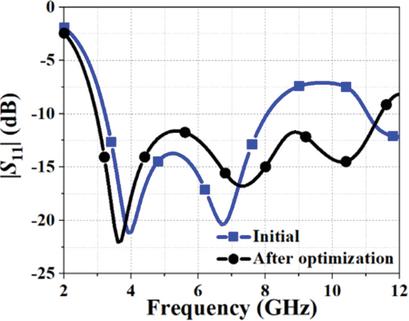
Figure 5 $| S_{11} |$ curve before and after optimization.

The optimized structural parameters of UWB antenna are shown in Table 1. The overall geometry is fabricated with Printed Circuit Board (PCB) technology, and is shown in Fig. 6.

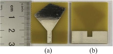
Figure 6 Photograph of the fabricated antenna: (a) top view and (b) bottom view.

The scattering parameters of the antenna were measured using a vector network analyzer. Figure 7 compares the simulated and measured $| S_{11} |$ results. Overall, the measured data show good agreement with the simulations, and the operating frequency bands are consistent. Slight discrepancies are observed at 6 GHz and 8 GHz, which can be attributed to differences between the actual and modeled substrate properties, such as the relative dielectric constant and loss tangent of FR4, as well as the effect of the longer coaxial feeding cable used during measurements. These factors do not affect the overall validation of the antenna performance.

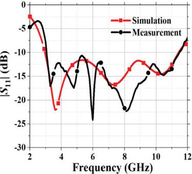
Figure 7 $| S_{11} |$ curve of the UWB antenna.

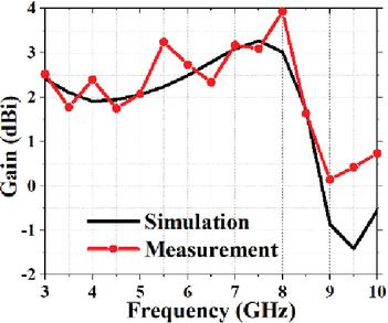
Figure 8 Gain curves of the UWB antenna.

The radiation pattern and gain curve of the UWB antenna are tested in a microwave anechoic chamber. When this antenna works in the frequency range of 3 to 10 GHz, the gain curve obtained from the test is shown in Fig. 8, and the test value is roughly consistent with the simulation value. There are some fluctuations for the measured gain. We measured the gain of each frequency separately with the standard horn antenna and the far-field test system. A gain error of $\pm$ 0.5 dB for test system and testing environment, these will have an impact on the measured gain results. At 5.0 GHz, the normalized XOZ- and YOZ-plane radiation directions of the UWB antenna are shown in Figs. 9 (a) and 9 (b). Similarly, the normalized XOZ- and YOZ-plane radiation directions of the UWB antenna at 7 GHz are shown in Figs. 9 (c) and 9 (d), respectively. There are some differences between simulation and measurement, especially in the XOZ plane. This is mainly caused by the addition of SMA connectors at the antenna feed and the test cable being located on the back of the antenna during testing. In general, the test results and simulation results maintain similar radiation patterns and have the same cross polarization level values. The measured results are in good agreement with the simulation results. Since the focus of this paper is to optimize the S-parameters of the antenna, only the radiation pattern of one frequency is given here.

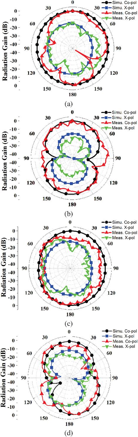
Figure 9 2D radiation patterns of the fabricated antenna: (a) XOZ-plane @5 GHz, (b) YOZ-plane @ 5 GHz, (c) XOZ-plane @ 7 GHz, (d) YOZ-plane @ 7 GHz.

Table 2 Comparison of the performance of UWB antennas ( $f_{0}$ is the center frequency)

Ref.	Operation Frequency Band (GHz)	Type	$f_{0}$ (GHz) Size $(λ_{0})$	Peak Gain (dBi)
[24]	3.4–9	Monopole	6.2 0.83 $\times$ 0.83 $\times$ 0.03	/
[25]	1.55–17.6	Slot	9.575 6.38 $\times$ 6.38 $\times$ 0.03	10.2
[26]	2.95–10.8	MIMO	6.875 1 $\times$ 1 $\times$ 0.04	4.0
[27]	2.1–11.5	Slot	6.8 1.15 $\times$ 1.15 $\times$ 0.03	5.8
This Work	2.95–11.43	Monopole	7.19 0.72 $\times$ 0.65 $\times$ 0.04	4.0

In conclusion, compared with the different UWB antennas that have been publicly reported, this design has significant advantages, such as small size and wide bandwidth, simplified design without complex feed network, and low manufacturing cost, which are shown in Table 2. Compared with the UWB antenna [24, 26], the proposed design has a broader working frequency band. Although the slot type antennas [25, 27] can have some advantages in operation frequency band, their large size brings many limitations to practical. The peak gain of proposed design is moderate, mainly due to the reduction in equivalent radiation area brought about by its miniaturized structure. In addition, the structure in this paper is simpler, the cost is easy to control, and there is no need for a feed network. This work can be a potential candidate for applications in UWB communication, positioning, and IoT systems.

4 ANOTHER EXAMPLE

To verify the effectiveness of the algorithm, a dual-band antenna is selected as the optimization objective. This antenna is of the same type as the UWB antenna mentioned earlier and both belong to patch antennas. Patch antennas [28, 29] have a wide range of applications and a relatively simple manufacturing process. It is meaningful to extend the optimization method combining GPR and GA to patch antennas.

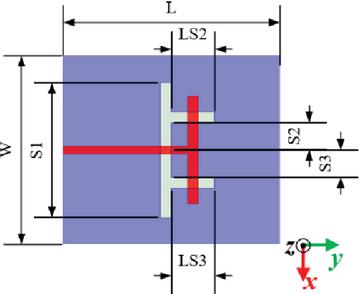
Figure 10 Geometry of the dual-band antenna.

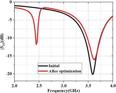
Figure 11 Performance of the dual-band antenna (S parameters).

The geometry of dual-band antenna is given in Fig. 10. The front of the antenna is a T-shaped patch, and the back is etched with $Π$ Type gap. The substrate is FR4 with a relative dielectric constant of 4.4 and a loss tangent of 0.02. The antenna has an overall size of 80 $\times$ 70 $\times$ 1.6 mm³. The optimization goal is to design the antenna as a dual band antenna, with two resonance frequencies of $f_{1} = 2.44$ GHz and $f_{2} = 3.62$ GHz, respectively. The proposed algorithm in above section is used to construct surrogate model and searching target, while the parameters of $L S_{2}$ , $L S_{3}$ , $S_{2}$ , and $S_{3}$ are used as the optimization variables. The initial values are: $L S_{2} = L S_{3} = 20$ mm, $S_{2} = S_{3} = 10$ mm. Obviously, the optimization goal can be other antenna performance. Similarly, 10 full-wave simulation data is collected as the initial dataset. The simulation frequency band is 2–4 GHz, step by 0.01 GHz, and each simulation has a total of 201 frequency points. A total of 10 simulations are 2010 data points. The comparison diagram of $S_{11}$ curves before and after final optimization is shown in Fig. 11. The optimized dual band antenna operates in the frequency bands of 2.44–2.46 GHz and 3.50–3.74 GHz and can be applied to WiFi and 5G. The corresponding parameters are $L S_{2} = 11$ mm, $L S_{3} = 19$ mm, $S_{2} = 8$ mm, $S_{3} = 9$ mm. The normalized radiation patterns at 2.45 GHz and 3.6 GHz are also given in the Fig. 12. The cross-polarization curves are also added for evaluating the performance in Figs. 12 (a) and 12 (b), which shows cross polarization levels of more than 10 dB at two different frequencies. The proposed dual-band antenna exhibits stable broadside radiation, and two radiation nulls at YOZ plane. The algorithm is repeated 5 times on the same initial dataset, and the average optimization time is 277.47 seconds. This indicates that the optimization scheme combining GA and GPR can facilitate and quickly design antenna structures.

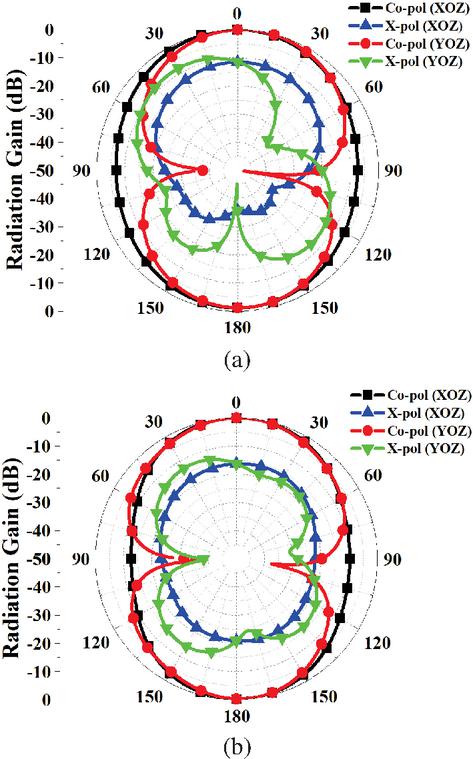
Figure 12 2D radiation patterns of the simulated antenna: (a) 2.45 GHz and (b) 3.6 GHz.

5 CONCLUSION

In this paper, a complete optimization scheme is designed by using the GPR and GA. After only 7 iterations, the optimization design of a UWB antenna with irregular patches is completed. In this optimization design, the average time to complete one iteration is 41 seconds. The optimization took a total of 601 seconds, including the time of initial 10 full-wave electromagnetic simulations (314 seconds) to collect the initial sample set and the time of 7 iterations. Then the optimization algorithm is carried, and the design target can be achieved with 7 iterations. Among each iteration, the time of full-wave electromagnetic simulation is 31.4 seconds, the time of the training GPR model is118 milliseconds, the trained GPR model has 6 input variables, and each generation of GA with a population size of 50 needs about 185 milliseconds.

The optimized UWB antenna has an operating band of 2.95–11.43 GHz, a relative bandwidth of 117.94%, and a physical size of only 30 $\times$ 27 $\times$ 1.6 mm³ (length $\times$ width $\times$ height). The patch of the antenna exhibits an irregular polygonal structure, highlighting how algorithm optimization not only enhances design efficiency but also facilitates the creation of innovative structures. Finally, the designed antenna is fabricated and tested. The measured frequency band and radiation direction are in good agreement with the simulated values. The effectiveness of the ML algorithm in UWB antenna design is proved.

ACKNOWLEDGMENT

This work is supported partly by “Pioneer” and “Leading Goose” R&D program of Zhejiang under contract of 2022C01119, partly by the National Natural Science Foundation of China under Contract of 62171169, partly by Project of State Key Laboratory of Millimeter Waves under contract of K202414.

REFERENCES

[1] J. Y. Park and J. Choo, “Zigzag antenna design based on machine learning,” Applied Computational Electromagnetics Society (ACES) Journal, vol. 40, no. 01, pp. 20–25, Jan. 2025.

[2] J. Dou, “Convolutional neural networks aided reinforcement learning for accelerated optimization of antenna topology,” Applied Computational Electromagnetics Society (ACES) Journal, vol. 40, no. 01, pp. 35–41, Jan. 2025.

[3] Y. Chen, V. Demir, S. Bhupatiraju, A. Z. Elsherbeni, J. Gavilan, and K. Stoynov, “Prediction of antenna performance based on scalable data-informed machine learning methods,” Applied Computational Electromagnetics Society (ACES) Journal, vol. 39, no. 04, pp. 275–290, Apr. 2024.

[4] E. Demircioglu, M. H. Sazlı, S. Taha İmeci, and O. Sengul, “Soft computing techniques on multi-resonant antenna synthesis and analysis,” Microwave and Optical Technology Letters, vol. 55, no. 11 pp. 2643–2648, Nov. 2013.

[5] L. W. Mou, Y. J. Cheng, Y. F. Wu, M. H. Zhao, and H. N. Yang, “Design for array-fed beam-scanning reflector antennas with maximum radiated power efficiency based on near-field pattern synthesis by support vector machine,” IEEE Transactions on Antennas and Propagation, vol. 70, no. 7, pp. 5035–5043, July 2022.

[6] D. R. Prado, P. Naseri, J. A. López-Fernández, S. V. Hum, and M. Arrebola, “Support vector regression-enabled optimization strategy of dual circularly-polarized shaped-beam reflectarray with improved cross- polarization performance,” IEEE Transactions on Antennas and Propagation, vol. 71, no. 1, pp. 497–507, Jan. 2023.

[7] X. W. Dai, D. L. Mi, H. T. Wu, and Y. H. Zhang, “Design of compact patch antenna based on support vector regression,” Radioengineering, vol. 31, no. 3, pp. 339–345, Sep. 2022.

[8] S. Koziel, N. Çalık, P. Mahouti, and M. A. Belen, “Accurate modeling of antenna structures by means of domain confinement and pyramidal deep neural networks,” IEEE Transactions on Antennas and Propagation, vol. 70, no. 3, pp. 2174–2188, Mar. 2022.

[9] A. M. Montaser and K. R. Mahmoud, “Deep learning-based antenna design and beam-steering capabilities for millimeter-wave applications,” IEEE Access, vol. 9, pp. 145583–145591, 2021.

[10] L. Cui, Y. Zhang, R. Zhang, and Q. H. Liu, “A modified efficient KNN method for antenna optimization and design,” IEEE Transactions on Antennas and Propagation, vol. 68, no. 10, pp. 6858–6866, Oct. 2020.

[11] J. Jacobs and J. de Villiers, “Modeling of planar dual-band microstrip patch antenna using Gaussian process regression,” in The 3rd European Wireless Technology Conference, Paris, France, pp. 253–256, 2010.

[12] J. P. Jacobs, “Efficient resonant frequency modeling for dual-band microstrip antennas by Gaussian process regression,” IEEE Antennas and Wireless Propagation Letters, vol. 14, pp. 337–341, 2015.

[13] B. Woosley, J. Twigg, J. G. Rogers, and F. Dagefu, “Learning antenna radiation patterns through Gaussian process regression,” in 2022 IEEE International Symposium on Antennas and Propagation and USNC-URSI Radio Science Meeting (AP-S/URSI), Denver, CO, USA, pp. 637–638, 2022.

[14] H. Ibili, A. C. Gungor, M. Maciejewski, J. Smajic, and J. Leuthold, “Genetic algorithm-based geometry optimization of terahertz plasmonic modulator antennas,” in 2022 23rd International Conference on the Computation of Electromagnetic Fields (COMPUMAG), Cancun, Mexico, pp. 1–4, 2022.

[15] K. Choi, D.-H. Jang, S.-I. Kang, J.-H. Lee, T.-K. Chung, and H.-S. Kim, “Hybrid algorithm combing genetic algorithm with evolution strategy for antenna design,” in IEEE Transactions on Magnetics, vol. 52, no. 3, pp. 1–4, Mar. 2016.

[16] A. J. Kerkhoff and H. Ling, “Design of a band-notched planar monopole antenna using genetic algorithm optimization,” IEEE Transactions on Antennas and Propagation, vol. 55, no. 3, pp. 604–610, Mar. 2007.

[17] X.W. Dai, W. H. Hu, Y. H. Fu, J. Liu, and Z. X. Chen, “Automatic design of microwave filters by using relational induction neural networks,” Int. J. Numer. Model, vol. 36, no. 6, e3102, 2023.

[18] J. P. Jacobs and J. P. de Villiers, “Gaussian-process-regression-based design of ultrawide-band and dual-band CPW-FED slot antennas,” Journal of Electromagnetic Waves and Applications, vol. 24, no. 13, pp. 1763–1772, 2012.

[19] A. Pietrenko-Dabrowska, S. Koziel, and M. Al-Hasan, “Cost-efficient bi-layer modeling of antenna input characteristics using gradient Kriging surrogates,” IEEE Access, vol. 8, pp. 140831–140839, 2020.

[20] A. Pietrenko-Dabrowska and S. Koziel, “Simulation-driven antenna modeling by means of response features and confined domains of reduced dimensionality,” IEEE Access, vol. 8, pp. 228942–228954, 2020.

[21] S. Koziel and A. Pietrenko-Dabrowska, “Reliable data-driven modeling of high-frequency structures by means of nested Kriging with enhanced design of experiments,” Engineering Computations, vol. 36, no. 7, pp. 2293–2308, 2019.

[22] A. Pietrenko-Dabrowska and S. Koziel, “Reliable surrogate modeling of antenna input characteristics by means of domain confinement and principal components,” Electronics, vol. 9, no. 5, p. 877, 2020.

[23] T. O. Kvålseth, “Cautionary note about R²,” The American Statistician, vol. 39, no. 4, pp. 279–285, 1985.

[24] M. N. Hasan and M. Seo, “A planar 3.4–9 GHz UWB monopole antenna,” in 2018 International Symposium on Antennas and Propagation (ISAP), Busan, Korea (South), pp. 1–2, 2018.

[25] Y. Wang and W. Dou, “A low profile UWB antenna on a large flat conductor,” in 2021 International Symposium on Antennas and Propagation (ISAP), Taipei, Taiwan, pp. 1–2, 2021.

[26] Y.-Y. Liu and Z.-H. Tu, “Compact differential band-notched stepped-slot UWB-MIMO antenna with common-mode suppression,” IEEE Antennas and Wireless Propagation Letters, vol. 16, pp. 593–596, 2017.

[27] P. M. Paul, K. Kandasamy, M. S. Sharawi, and B. Majumder, “Dispersion-engineered transmission line loaded slot antenna for UWB applications,” IEEE Antennas and Wireless Propagation Letters, vol. 18, no. 2, pp. 323–327, Feb. 2019.

[28] B. Tutuncu, H. Torpi, and S. Taha Imeci, “Directivity improvement of microstrip antenna by inverse refraction metamaterial,” Journal of Engineering Research, vol. 7, no. 4, pp. 151–164, Dec. 2019.

[29] S. Salihovic and S. Taha Imeci, “A stub microstrip patch antenna for sub 6 GHz – 5G applications,” Heritage and Sustainable Development Original Research, vol. 5, no. 1, pp. 99–106, June 2023.

BIOGRAPHIES

Da Li Mi was born in Haining, Zhejiang, China. He received his master’s degree in electronic information from Hangzhou Dianzi University, Hangzhou, Zhejiang, in 2023. His current interests include artificial intelligence, antennas, and electromagnetic compatibility.

Xi Wang Dai was born in Caoxian, Shandong, China. He received the B.S. and M.S. degrees in Electronic Engineering from Xidian University, Xi’an, Shanxi, in 2005 and 2008, and he received the Ph.D. degree in Electromagnetic Fields and Microwave Technology from Xidian University in 2014. From March 2008 to August 2011, he worked at Guangdong Huisu Corporation as a manager of the antenna department. He currently works at Hangzhou Dianzi University, Hangzhou. His current research interests involve metamaterials, AI-assisted design antenna, MIMO antenna and low-profile antenna.

Jun Shi Zhao was born in Zhoukou, Henan, China. He received the B.S. degree in Electronic Information Engineering from Xi’an Shiyou University, Xi’an, Shanxi, in 2023. He is currently pursuing the master’s degree with Hangzhou Dianzi University, Hangzhou, Zhejiang. His current research interests include broadband antenna and microstrip antenna.

Ze Li was born in Wenzhou, Zhejiang, China, in 2001. He received the B.S. degree in electronic information engineering from Hangzhou Dianzi University Information Engineering College, Hangzhou, in 2023. He is currently pursuing the M.S. degree in the Hangzhou Dianzi University, Hangzhou. His current research interests include orbital angular momentum and metasurface antenna.

Gang Li was born in Suizhou, Hubei, China. He received the B.S. degrees in electronic engineering from Xidian University, Xi’an, Shaanxi, in 2005, and the Ph.D. degree in electromagnetic fields and microwave technology at Xidian University in 2009. From May 2010 to August 2012, he worked at Huawei Technologies Co. Ltd. as an EMC Engineer. He currently works at Hubei University of Arts and Science, Xiangyang. His current research interests involve broadband antenna, RCS and metasurface.

Hui Hong received the Ph.D. degree in electronic science and technology from the College of Information Science & Electronic Engineering, Zhejiang University, Hangzhou, China, in 2007. Currently, he is a Full Professor with the School of Electronics and Information Engineering, Hangzhou Dianzi University, Hangzhou. His research interests include brain–computer interface, microsystem integration, and biological signal processing.