Optimizing Multi-coil Integrated High-speed On/Off Valves for Enhanced Dynamic Performance with Voltage Control Strategies
Shuai Huang and Hua Zhou
1State Key Laboratory of Fluid Power and Mechatronic Systems
Zhejiang University, Hangzhou 310058, China
12225110@zju.edu.cn, hzhou@zju.edu.cn
2Mechanical Engineering Department
Jiangxi Polytechnic University, Jiujiang 332007, China
Submitted On: July 13, 2024; Accepted On: December 6, 2024
ABSTRACT
In optimizing high-speed on/off valves (HSVs), key components of digital hydraulic systems, this study introduces a method designed for multi-coil integrated HSVs, differing from the traditional focus on single-coil solenoid configurations. The proposed method is an optimization framework that matches with voltage control strategies to significantly enhance the dynamic performance of HSVs. Through the integration of simulation and experimental analyses, the investigation explores the functional relationship among coil volume, temperature rise, and input power. Additionally, utilizing multi-objective optimization (MOO) techniques to improve coil design and optimize performance based on meta-model of optimal prognosis (MOP) and evolution algorithm (EA), the results demonstrate that, when employing a three-voltage control strategy, coils designed with this strategy, compared to those with a single-voltage control strategy, significantly reduce the opening time for normally closed (NC) and normally open (NO) valves by up to 40% (from 5.0 ms to 3.0 ms) and 36.4% (from 5.5 ms to 3.5 ms).
Index Terms: Meta-model of optimal prognosis, multi-coil integrated, multi-objective optimization, optimization design match with control.
I. INTRODUCTION
Compared to electrohydraulic servo or proportional valves, digital valves offer several advantages, i.e. anti-oil contamination, low throttling losses, low cost, and better performance in small system drives or actuators [1–3]. Many studies have reported on digital valves that use multiple high-speed on/off valves (HSVs) as a piloted stage or in parallel connection, instead of proportional slide valves, to improve energy efficiency and reduce costs [4]. As the key element of digital valves, HSV face several challenges, including rapid response, temperature rise control, and miniaturization [5, 6].
The rapid response of HSVs, while allowing for a permissible temperature rise, is a key factor in enhancing the response speed and control performance of digital hydraulic systems [7, 8]. During the design stage of HSVs, many studies have focused on optimizing key structural parameters to improve performance [9]. Liu et al. [10] analyzed the effects of key parameters, such as the armature, pole shoe, coil, and drive current, on the electromagnetic force of HSVs. Lantela and Pietola [11] developed a digital hydraulic valve system consisting of numerous micro-HSVs connected in parallel. Through system optimization, the response speed was reduced to approximately 2 ms. Li-mei et al. [12] used genetic algorithms (GA) to optimize parameters such as the coil turns, spring preload and stiffness, armature mass, and air gap of the HSV, in order to improve its response speed. Wu et al. [6] adopted a multi-objective optimization (MOO) method to determine the key parameters of the HSV, targeting the opening and closing times. They employed particle swarm optimization (PSO) and the analytic hierarchy process (AHP) principles, building upon the conventional single-voltage approach. Zhong et al. [13] optimized seven main geometric parameters of the HSV using the magnetic equivalent circuit (MEC) method, with the goal of achieving optimal dynamic performance and minimizing volume, based on GA. Sudhoff [14] optimized the coil of the EI-type solenoid using both the MEC and thermal equivalent circuit (TEC) model. Additionally, to improve the optimization efficiency of the HSV, an optimization approach based on surrogate model was also employed [15–17].
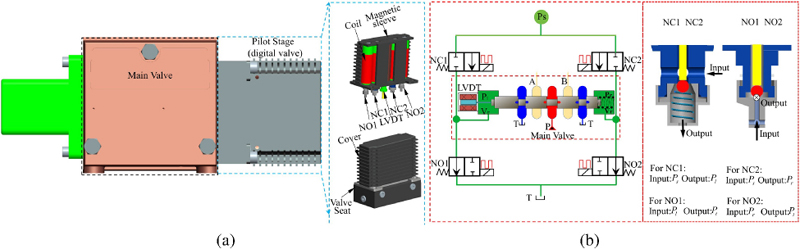
Figure 1: Principle and structure of the digital valve: (a) three-dimensional structural model and (b) principle of digital valves and valve port structure.
Upon completion of the design stage, an appropriate voltage control strategy is optimized to improve the performance [18]. To address issues such as high-power consumption and long closing delays in single-voltage control, Taghizadeh et al. [19] developed an improved method using dual voltages, applying a low voltage during the hold stage of the HSV to reduce power consumption and effectively minimize shutdown delay times. Furthermore, dual voltage strategies do not effectively reduce the impact of magnetic hysteresis on closing delays. Lee et al. [20] developed a three-voltage control strategy that addresses the delay caused by magnetic hysteresis by applying a reverse voltage during the closing phase. The experiments indicate a reduction in closing delay time from 5 ms to 1.55 ms. Additionally, to accommodate variations in hydraulic pressure and enhance control flexibility, Zhang et al. [21] proposed a PWM-based adaptive three-voltage control strategy, which automatically adjusts the PWM duty cycle based on oil pressure to ensure consistent opening and closing times of the HSV, regardless of changes in oil pressure. Furthermore, frequent high-speed opening and closing can shorten the operational lifespan of the HSV. Gao [22] designed a compound voltage control strategy based on three-voltage, using a negative voltage during the opening stage of the HSV to reduce the collision velocity between the ball and the seat, thereby extending the lifespan of the HSV.
So far, most studies on HSVs have focused on single-coil solenoid structures. There is limited research on the dynamic and thermal performance of HSVs with multi-coil integrated non-solenoid structures. Furthermore, a significant amount of research has been conducted on this subject, with a primarily focus on optimizing the parameters of the HSV’s structure under single-voltage control. Subsequently, improvements have been made to the voltage control strategy during the control stage, with each aspect developed independently. However, few studies have focused on the potential impact of voltage control strategies on optimizing coil parameters to enhance dynamic performance.
The parameters of the coil play a key role in influencing the dynamic characteristics of HSV [10]. Thus, the aim of this paper is to improve the dynamic performance of the HSV during the design stage by optimizing the coil parameters in conjunction with voltage control strategies, specifically in the context of the multi-coil integrated digital valve. The main contributions of this article are summarized as follows.
(1) An optimization approach for multi-coil integrated non-solenoid structures HSVs is proposed, based on the meta-model of optimal prognosis (MOP) and evolutionary algorithm (EA).
(2) This paper presents a coil design method based on a matched voltage control strategy, considering the effects of temperature rise.
The structure of this article is organized as follows. Section II briefly describes the structure of the digital valve. In section III, a theoretical model for the HSV is developed. The detailed steps and process for the optimization design based on the voltage control strategy are conducted in section IV. The practical performance of the HSV is evaluated under various voltage control strategies. Additionally, an in-depth analysis and discussion of the experimental results are presented in section V. Finally, section VI draws a conclusion and discusses the future work.
II. STRUCTURE OF THE DIGITAL VALVE
As shown in Fig. 1, the digital valve, which controls the main valve, primarily consists of four valve bodies of the HSVs, four coils, a magnetic sleeve, thermal grease, and a linear variable differential transformer (LVDT) [23]. In this study, NC1 and NC2 are two-position, two-way normally closed valves that use a spring for resetting. When the coil is energized, the electromagnetic force moves the ball downward, causing the HSV to open. Conversely, when the coil is de-energized, the spring returns the ball assembly upward, closing the HSVs. In contrast to NC1 and NC2, the internal structure of the normally open valves (NO1 and NO2) eliminates the spring component, and the reset process primarily relies on the hydraulic pressure acting on the ball.
III. DEVELOPMENT OF THEORETICAL MODELS
A. Modeling of the magnetic circuit
Symbol definitions are as follows for developing an EMC model for the digital valve. R represents the magnetic reluctance, where i refers to the number of reluctances and denotes various components of the HSV. a denotes armature, b means valve body, g means air gap, s means magnetic sleeve, and p denotes pole shoe. Since the permeability of the cover is similar to that of air, both the cover and the air are treated as a single medium for calculation purposes.
The magnetic path model is segmented into six parts, as illustrated in Fig. 2.
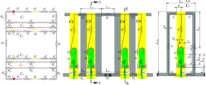
Figure 2: Geometric illustration and corresponding magnetic circuit model of the digital valve.
The reluctances of the magnetic frame can be expressed using equations (1)-(4):
| (1) | ||
| (2) | ||
| (3) | ||
| (4) |
The reluctance of the air gap can be calculated by equations (5) and (6):
| (5) | ||
| (6) |
The reluctances of other parts can be calculated by equations (7)-(10):
| (7) | ||
| (8) | ||
| (9) | ||
| (10) |
The reluctances of the magnetic circuit is presented in equations (11)-(14):
| (11) | ||
| (12) | ||
| (13) |
| (14) |
where R, R, R, and R are the reluctances of C, C, C, and C, respectively. C represents the magnetic circuit branch of NO1. C denotes the magnetic circuit branch of the magnetic sleeve at the J-J sectional plane. C represents the magnetic circuit branch of NC1. C depicts the magnetic circuit branch of the magnetic sleeve at the K-K sectional plane.
The structural parameter values required for the aforementioned magnetic reluctance calculations are specified as follows: r 4 mm, r 2.75 mm, r 2.8 mm, L 34 mm, L 15.6 mm, L 10 mm, L 12.1 mm, L 8.15 mm, L 16 mm, L 27 mm, L 32 mm, L 20 mm, L 57.2 mm, L 12 mm, t 3 mm, a 0.5/0.15 mm (de-energized state/ energized state).
It can be seen from Fig. 2 that magnetic field of NO1 mainly flows through the paths of C, C, R, C, and R, while the magnetic lines of force of NC1 mainly flow through the paths of C, C,R, C, and R. Therefore, the total magnetic resistance of NC1 and NO1 can be expressed as:
| (15) | |
| (16) |
The electromagnetic force acting on the HSV can be formulated as [21]:
| (17) |
where is air permeability, S is the cross-section area of armature, and is a constant related to the leakage magnetic flux.
The magnetic circuit model of the HSV can be expressed as:
| (18) |
B. Mathematical model of mechanical field
During the opening and closing stages of the HSV, the moving components experience the combined influence of electromagnetic force, hydraulic force, hydrodynamic force, spring force, and damping force. As a result, its dynamic equation can be formulated as [7] for NC1, NC2:
| (19) |
For NO1, NO2:
| (20) |
where m is the mass of the armature, F represents the electromagnetic force of the solenoid, F and F denote the transient and steady-state hydrodynamic forces, respectively, B is the damping coefficient, and P is the pilot oil pressure. For NC1 and NO1, P P. For NC2 and NO2, P P. A is the cross-sectional area of the port and k is the stiffness of the spring for NC1 and NC2.
When the HSV operates in a static state, the terms dx/dt and dx/dt all equal zero. Additionally, neglecting transient hydrodynamics, the critical electromagnetic force can be further defined as [7] for NC1, NC2:
| (21) | ||
| (22) |
where P is the pressure differential between the input and output ports of NC1 and NC2, x is the precompression of the spring, a is the working stroke of the armature, Cis the fluid velocity coefficient, C is the flow coefficient, is the flow angle, and A is the open area of orifice.
For NO1, NO2:
| (23) | ||
| (24) |
where P is the pressure difference between the input and output port of the NO1 and NO2.
Based on equations (17), (18), and (21)-(24), the opening and closing current of the HSV can be calculated by the equations (25)-(28) for NC1, NC2:
| (25) | ||
| (26) |
For NO1, NO2:
| (27) | ||
| (28) |
The number of turns N can be expressed as a function of the winding dimensions:
| (29) |
where f is the coil stacking factor, based on practical experience, which is fixed as 0.65. d and d are the outer and inner diameters of the winding, respectively, l is the length of the winding, and dis the diameter of the copper wire.
From [13], it is known that the opening and closing times are mainly affected by the coil resistance, the number of turns, the supply voltage, and the voltage control strategy under the same structural parameters of solenoid. These parameters also affect the coil’s resistance loss, which in turn leads to different temperature rises in the digital valve.
C. Voltage control strategies for HSV
The flowchart of voltage control is shown in Fig. 3, which illustrates the control flow for both single-voltage and three-voltage control strategies [21].
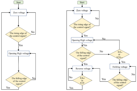
Figure 3: Flowchart of different voltage control strategies: (a) single-voltage control and (b) three-voltage control.
Assuming the voltage, duty ratio, and frequency of the control signal are 5 V, 0.5, and 50 Hz, respectively, the opening voltage, holding voltage, and reverse voltage are 24 V, 5 V, and -24 V, respectively. The profiles of the drive voltage and the control signal for the HSV are depicted in Fig. 4.
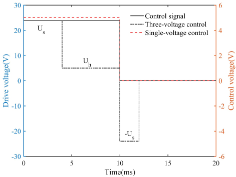
Figure 4: Profile of the drive voltage for HSV.
The most notable distinction between the three- voltage and single-voltage control strategies lies in their mechanisms for adjusting the coil excitation voltage: once the valve reaches the end position, the excitation voltage is adjusted to U. Furthermore, when the falling edge of the control signal is detected, the coil’s excitation voltage is switched to -U:
| (30) |
where n is the safety factor, typically taken as 1.05-1.1. Uis the holding voltage and I is the closing current which is expressed in equations (26) and (28). The resistance of the coil can be calculated as:
| (31) |
where is the resistivity of the copper and d is the bare diameter of the copper wire.
The power generated by the coil is influenced by the choice of voltage driving strategies [13]. Therefore, by applying different voltage control strategies and considering the temperature rise limitations, it is possible to determine the optimal coil parameters for the HSV.
IV. OPTIMIZATION OF COIL DESIGN GUIDED BY VOLTAGE DRIVING STRATEGY ALIGNMENT
A. Modelling of temperature rise
The normally open (NO) and normally closed (NC) valves on the same side constitute a pair of two-way, three-way valves. To improve the positioning control accuracy of the main valve, the differential PWM (D-PWM) control method is commonly adopted [24]. In each control period, power needs to be supplied to four coils. Analysis of the coil’s temperature rise is required under the condition of simultaneously supplying power for four coils. Furthermore, the temperature rise characteristics of the digital valve are dependent on the coil volume and input power. For precise determination of the integrated coil temperature rise, this study adapts finite element simulation and experimental validation methodologies to obtain the “power-volume-temperature rise” characteristics of the integrated multi-coil.
The steady-state thermal distribution of the digital valve is analyzed using the steady-state thermal simulation module in ANSYS Workbench. The finite element matrix form of the steady-state heat balance equation is [14, 25]:
| (32) |
where [C] represents the specific heat matrix, [K] represents the conduction matrix, which is related to material properties and geometry, [K] represents the convection matrix, [T] represents the nodal temperature vector, and Q represents the heat generation vector, including the Joule heating P generated by the current passing through the coil. Joule heat is the heat produced by the current flowing through the conductor and is transferred to the various components via thermal conduction. Q represents the convection heat vector which can be calculated using the following formula:
| (33) |
where h represents the convective heat transfer coefficient, S is the projected area of the element surface in the direction normal to its interface with the environment, and T represents the ambient temperature.
The ambient temperature is set as 25 in the simulation model. The coil section is equivalently treated as a homogeneous entity [26]. The dimensions of the coil were set as follows: d 11.5 mm, d 14.0 mm, l 40 mm. Joule heating of the four coils was set as the heat source. To enhance computational efficiency, the four HSVs are simplified to a cylindrical shape, with the fins on the cover being neglected. Energy radiation heat transfer is turned off, and the direction of gravity is set along the y-axial. Convection, a heat transfer phenomenon in a fluid medium, depends on the geometric arrangement, temperature, and properties of the convective medium surrounding the surface [27], and can be calculated by equation (34):
| (34) |
where thermal conductivity, set as for air, acceleration due to gravity, set as volumetric thermal expansion coefficient, set as temperature difference between the surface of the object and the air, and empirical constant, kinematic viscosity, set as , and characteristic length.
If the outer face of the digital valve, whose normal are parallel to the direction of gravity, then L can be expressed as:
| (35) |
where S and p is the area and the perimeter of the plane surface, respectively.
Prandtl number P can be expressed as:
| (36) |
where specific heat capacity at constant pressure, set as , and dynamic viscosity, set as
The material parameters of each component are shown in Table 1.
Table 1: Thermal parameters of parts
| ThermalParameters | Density(kg/m) | Specific Heat Capacity | ThermalConductivity |
| Copper | 8978 | 381 | 378.6 |
| Air | 1.16 | 1007 | 0.026 |
| Bracket/HSV | 7870 | 460 | 80 |
| Shell | 1400 | 1150 | 0.25 |
| Bobbin | 1420 | 1150 | 0.24 |
| Grease | 1500 | 2300 | 1.5 |
| Valve seat | 2770 | 875 | 165 |
The temperature distribution under varying power does not include the cover and thermal grease in Fig. 5. In Fig. 5 (a), each coil was subjected to a power input of 4.35 W. The simulation results indicated that the maximum temperature of coil NO1 reached 107.74C, corresponding to a temperature rise of 82.74C. Additionally, each coil was subjected to a power input of 5.52 W in Fig. 5 (b). The results show that the maximum temperature of coil NO1 reached 126.22C, corresponding to a temperature rises of 101.22C.
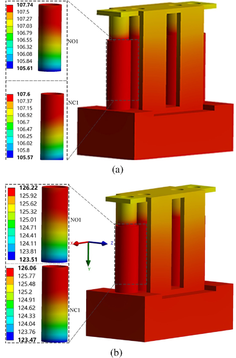
Figure 5: Temperature results under different power input: (a) power input of 4.35 W and (b) power input of5.52 W.
A test bench was developed to validate the finite element simulation results. The coil dimensions were kept the same as those used in the simulation, with an ambient temperature set to 25C. The temperature rise of the coil was measured using the resistance method, employing the test setup depicted in Fig. 6. The current in the winding of the HSV was detected using a CHB-2AD closed-loop Hall current sensor, and its voltage signal output was collected by an STM32F103ZET6 control board. Measurements were taken at intervals of 0.25 seconds until the temperature reached a steady state.
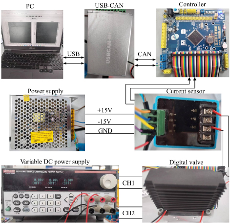
Figure 6: Experimental setup for testing temperature rise of the digital valve.
From Fig. 7, it is evident that the maximum relative error between the simulation results and the experimental data is approximately 11% at an input power of around 3 W, with the majority of the data points exhibiting an error of less than 10%. This confirms the reliability of the simulation model settings.
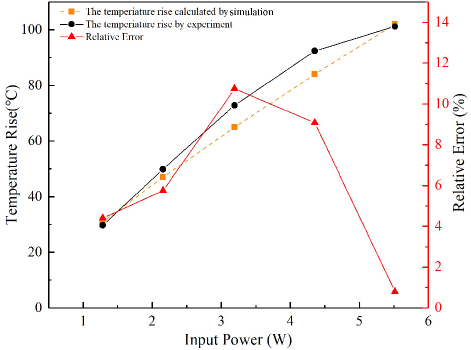
Figure 7: Comparison of temperature rise between the experiment and simulation.
To research the function relationship between input power, coil temperature rise, and coil volume for NO1, the coil’s outer diameter dranged from 12.5 mm to 14.2 mm, with intervals of 0.5 mm; the coil height l ranged from 20 mm to 45 mm, with intervals of 5 mm. The input power ranged from 1 W to 9 W, with intervals of 1 W. Temperature rise data points for coil NO1 were then obtained under these various conditions. Finally, the black data points in Fig. 8 represent the results obtained through simulation.
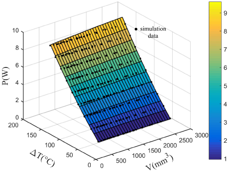
Figure 8: Temperature rise characteristic surface of NO1.
We use the matching tool in MATLAB software to fit the simulation data. The surface shown in Fig. 8 is fitted to equation (37), and the coefficients of the expression for P(V,T) are determined by equation (37):
| (37) |
where P(V, T) is the copper loss and V is the volume of the coil. T represents the temperature rise of the coil and is expressed by:
| (38) |
where T denotes the hotspot temperature of the NO1 and T represents the ambient temperature.
The fitting indicators, R and root mean squared error (RMSE) for equation (37) and Fig. 8 are 0.9998 and 0.04163, respectively. These metrics assess the accuracy and reliability of the mathematical expression in equation (37).
In addition, the results of the variance analysis of the coil temperature rise data points indicate that the coil temperature rise (T) has the greatest impact on input power, followed by the square of the coil temperature rise (T), then the coil volume (V), and the interaction term between coil volume and temperature rise (VT) ranks last. Furthermore, combining the analysis from Fig. 8 and equation (37), it can be concluded that there is an approximately linear relationship between input power and coil temperature rise. Additionally, as the input power increases, the impact of coil volume on the coil’s temperature rise gradually becomes morepronounced.
B. Multi-objective optimization
In the present study, the designed stroke of armature is a 0.35mm. The design parameters for the proposed solenoid are shown in Fig. 2. The predefined parameters include inner diameter d 11.5 mm, initial air gap 0.5mm. The stiffness of the spring k 10N/mm, precompression x 0.7 mm. The external control signal operates at a frequency of 50Hz with a duty cycle of 0.5 [28]. When the main valve is controlled by D-PWM, it is found that when the main valve responds in step or sinusoidal tracking through Amesim/MATLAB co-simulation, the steady-state pressure in the left and right chambers is about 0.95Mpa. Thus, there are still four structure parameters that need to be optimized: l, d, d, and d, according to equations (29) and (31).
According to GB/T 7673.3-2008, the functional relationship between wire numbers (WNU),d and d is determined using a fitting method in MATLAB.
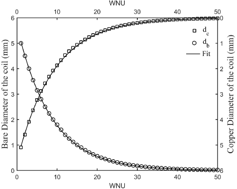
Figure 9: The relationship between the diameter of wire and WNU: (a) d and WNU and (b) d and WNU.
The fitting results are illustrated in Fig. 9. The R-square values for d and dare 0.9999 and 0.9997, respectively. and the RMSE for d and d are 0.00111 and 0.0227, respectively. The high accuracy of the fitting indicates the reliability of the fitted function. Therefore, there are three structure parameters in total that require optimization.
| (39) |
The MOP method uses sampling points to construct a surrogate model to replace the complex actual FEM model and implements an optimization algorithm based on MOP. The logic of the optimization process is outlined in Fig. 10.
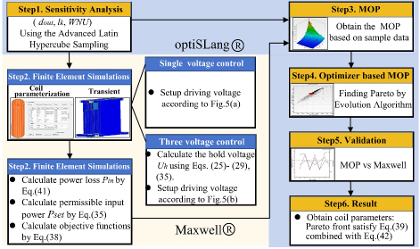
Figure 10: The optimization process of HSV in ANSYS Workbench.
Firstly, a sensitivity analysis is carried out. During this stage, according to the performance requirements of the HSV, we determine the parameters variables and range. Secondly, using the coil parameters obtained in the first step, we perform a transient finite element analysis to generate results under different voltage control strategies. Thirdly, we develop MOP based on the parameter variables, objectives, and constraints. Then, using MOP, we apply an EA to obtain the optimization results, which are subsequently validated in Maxwell.
In this study, the requirement of HSV is quick response. According to these requirements, we define the optimization objectives include opening time t and closing time t. All objectives will be calculated by equation (40).
Object functions:
| (40) |
Constraints: the allowable temperature rise of the coil shall not exceed 100C. Thus, the allowable input power should be computed using equation (37).
The simulation model integrates the following constraint functions:
| (41) |
where k is power loss ratio and u is parameter in the design vector. Its expression is:
| (42) |
If P is the copper power loss of the coil, the expression for it is:
| (43) |
where i is the current flowing through the coil and T is the period of the control signal.
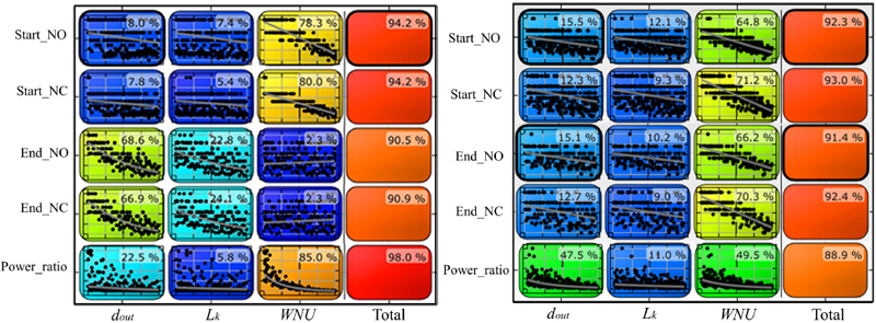
Figure 11: Full model CoPs: (a) single-voltage control and (b) three-voltage control.
The relevant parameters in this design study are given at: U 24 V, d[12.5 mm, 14.2 mm], l[20 mm, 45 mm], and WNU[26,40].
Latin hypercube sampling (LHS) is preferred for MOO due to its effective space-filling capabilities and independence among design variables [29]. Therefore, LHS was selected for subsequent analysis. Using LHS, 300 sample points were chosen, and the corresponding response values were computed for each point.
MOP involves fitting input and output variables using a mathematical model. However, for highly complex relationships, it cannot be guaranteed that the response surface will pass through all sample points. Therefore, analyzing the fitting accuracy is essential to ensure effective representation of the information contained in the original model. The Coefficient of Prognosis (COP) [30] is employed as a criterion to assess the accuracy of MOP.
All COPs are shown in Fig. 11. The COPs in the last column, which represent the full model, are all greater than 0.9. When COP0.7, this indicates strong fitting accuracy and supports the use of MOP as a viable alternative to the finite element method (FEM) in optimization [29]. From Fig. 11, it can be observed that WNU has a significant influence on the opening time of HSV, while the closing time is primarily influenced by changes in the diameter of the coil under single-voltage control.
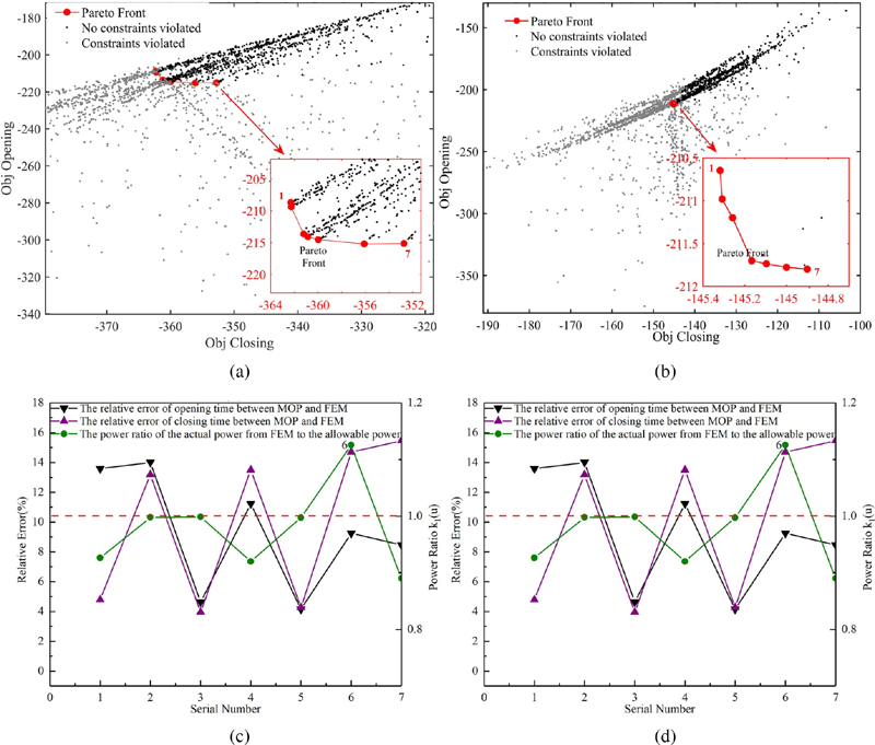
Figure 12: Optimization results based on MOP under single-voltage control: (a) relationship between the objective functions f(u) and f(u) for NC1, (b) relationship between the objective functions f(u) and f(u) for NO1, (c) relative error between MOP and FEM for NC1 and (d) relative error between MOP and FEM for NO1.
After obtaining the surrogate model in section B.3, this study adopted MOO using an EA based on the SPEA2 (Strength Pareto Evolutionary Algorithm 2) [31] to optimize the parameters of the coil, based on the criteria and constraints defined in section B.2. The parameters of the EA method are shown in Table 2 [32].
Table 2: Parameters of the evolutionary algorithm
| Name | Value | Name | Value |
| Maximum number of samples | 10000 | Selection method | Tournament |
| Population size | 10 | Crossover method | Simulated binary |
| Maximum number of generation | 1000 | Crossover probability | 0.5 |
| Fitness method | Pareto dominance | Mutation method | Self-adaptive |
| Constrain handling | Rank order | Mutation rate | 5% |
After a maximum of 10,000 function calls, the Pareto frontiers under different voltage control strategies were obtained.
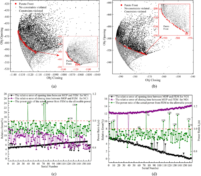
Figure 13: Optimization results based on MOP under three-voltage control: (a) relationship between the objective functions f(u) and f(u) for NC1, (b) relationship between the objective functions f(u) and f(u) for NO1, (c) relative error between MOP and FEM for NC1, and (d) relative error between MOP and FEM for NO1.
Figures 12 (a) and (b) show the Pareto 2D plots of the objectives under single-voltage control strategy. Gray represents particles that do not satisfy the constraints, black represents particles that satisfy the constraints, and the red line represents the Pareto frontiers, which includes the Pareto optimal solution set.
Figure 12 (a) denotes the relationship between the objective functions f(u) and f(u) for NC1. Figure 12 (b) represents the relationship between the objective functions f(u) and f(u) for NO1 under the single-voltage control strategy. There are seven points on the Pareto front. The optimization workflow ends with the validation of the MOP-based results presented in the Pareto front. The parameters of the coil obtained from MOP and located on the Pareto front were used as an input into Maxwell software to calculate the relative error in the coil’s opening time, closing time and power loss ratio compared to the predictions of the MOP.
As shown in Fig. 12 (c), under single-voltage control, the results obtained from MOP show a relative error of approximately 14% for NC1, 16% for NO1 in opening time, and 15% for NC1, 16% for NO1 in closing time, when compared to FEM.
One point (No. 6) does not meet equation (37) according to FEM results, as shown in Figs. 12 (c) and (d). Therefore, this point should be excluded in the subsequent calculations for the final optimal point.
Figure 13 (a) denotes the relationship between the objective functions f(u) and f(u) for NC1 underthree-voltage control strategy. Figure 13 (b) represents the relationship between the objective functions f(u) and f(u) for NO1. There are 163 points on the Pareto frontier under three-voltage control. As shown in Figs. 13 (c) and (d), under three-voltage control, the results obtained from MOP exhibit a relative error of approximately 8% for NC1, 10% for NO1 in opening time, and 14% for NC1 and NO1 in closing time, when compared to FEM. Twelve points fail to satisfy equation (37), as calculated from FEM, as depicted in Figs. 13 (c) and (d). Therefore, these points must be excluded from subsequent calculations for determining the final optimal point.
Under both single-voltage and three-voltage control strategies, the Pareto front data points have WNU of 34 and 31, respectively. This difference is likely due to the more significant impact of WNU on power loss compared to other design variables. Furthermore, the data points indicate a negative correlation between coil cross-sectional area and opening time (t), while a positive correlation is observed with closing time (t). A possible reason could be that, with a constant WNU, the coil cross-sectional area is positively correlated with the number of turns N, which in turn explains the observed correlation.
Table 3: Optimal coil parameters based on voltage control strategies
| Single-voltage | Three-voltage | ||||
| Experiment (ms) | Experiment (ms) | ||||
| Open | Close | Open | Close | ||
| Type A | NC1 | 5.0 | 4.0 | 5.0 | 1.5 |
| NO1 | 5.5 | 4.0 | 5.5 | 2.0 | |
| Type B | NC1 | / | / | 3.0 | 1.5 |
| NO1 | / | / | 3.5 | 2.0 |
There are numerous valid solutions that reside within the Pareto front. It remains challenging for designers to determine which solution to select. Therefore, methods must be applied to compare these solutions effectively [6]. In this paper, the optimal solution, which minimizes the value calculated using equation (44) is selected under the given constraint conditions:
| (44) |
The optimal solution for each voltage control strategy is listed in Table 3.
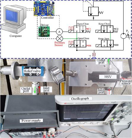
Figure 14: Experimental setup for testing the opening and closing times of HSV.
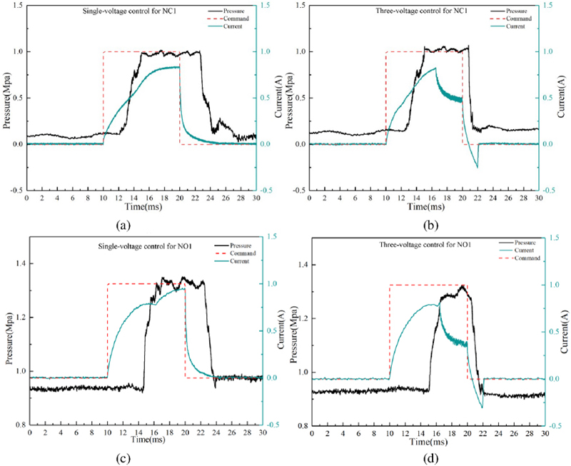
Figure 15: Experiment result of dynamic performance under type A coil for NC1 and NO1: (a)(c) single-voltage control and (b)(d) three-voltage control.
V. EXPERIMENTS
A. Experiments analysis
Several prototypes were fabricated, and a test bench was developed to measure the opening and closing times of the HSV. This test bench, shown in Fig. 14, uses a single pressure transducer to detect these times. The NO1 valve, connected to the tank, remains open as an orifice [6]. To reduce the pressure at the pump, a relief valve is installed between the inlet port of NC1 and the pump. NC1, which is connected to a pilot pressure source (1.35 MPa), is normally closed. The pressure transducer will detect the increment of the pressure. A current sensor (CHB-5AD) is used to detect the dynamic of the winding current. A driver (AIKONG AQMH2407ND) is developed to control the HSV which can generate voltage profiles required for single-voltage or three-voltage control. During the testing of NC1, NO1 is kept in a normally open state; conversely, when assessing NO1, NC1 is maintained in a continuously open condition.
From Fig. 15 (a), during the opening stage, the pressure curve shows that the HSV implements full opening within 5.0 ms. However, during the closing process, the current and pressure curves indicate that the HSV reaches full closure within 4.0 ms. In contrast to single-voltage control, using a three-voltage configuration results in a substantial reduction in the closing time of NC1, achieving full closure in less than 2.0 ms, as depicted in Fig. 15 (b). Regarding Fig. 15 (c), it is shown that the valve achieves full closure within 4.0 ms for NO1 during the closing stage. Simultaneously, during the opening process, both the current and pressure curves indicate that the valve reaches full opening within 5.5 ms. Similarly, implementing three-voltage control results in a significant reduction in the closing time of NO1 to less than 2.0 ms compared to single-voltagecontrol.
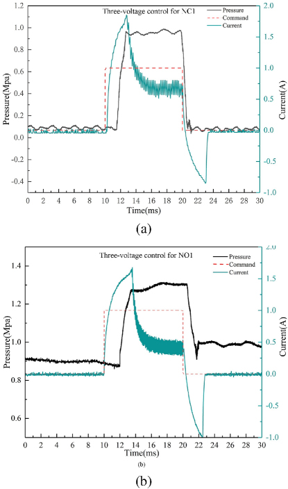
Figure 16: Experiment result of dynamic performance under type B coil for NC1 and NO1: (a) three-voltage control for NC1 and (b) three-voltage control for NO1.
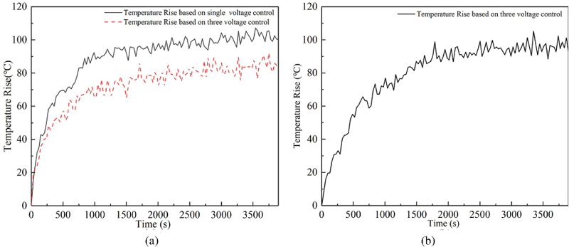
Figure 17: Curves depicting the temperature rise of the NO1 coil: (a) temperature rise of Type A coil under various voltage control strategies and (b) temperature rise of Type B coil under three-voltage control.
Table 4: Simulation and experiment results
| Single-voltage | Three-voltage | ||||
| Experiment (ms) | Experiment (ms) | ||||
| Open | Close | Open | Close | ||
| Type A | NC1 | 5.0 | 4.0 | 5.0 | 1.5 |
| NO1 | 5.5 | 4.0 | 5.5 | 2.0 | |
| Type B | NC1 | / | / | 3.0 | 1.5 |
| NO1 | / | / | 3.5 | 2.0 |
Based on Figs. 16 (a) and (b), the experimental results indicate that for NC1, the complete opening and closing times are approximately 3.0 ms and 1.5 ms, respectively. For NO1, the complete opening and closing times are approximately 3.5 ms and 2.0 ms, respectively.
From the experimental results in Figs. 15 and 16, it is evident that even with subsequent adoption of three-voltage control, the opening time of Type A coil cannot be reduced compared to the Type B coil. The specific data from the experimental findings are listed in Table 4.
From Table 4, it is shown that when both coils adopt the three-voltage control strategy, the Type B coil significantly reduces the opening time for NC and NO by up to 40% (from 5.0 ms to 3.0 ms) and 36.4% (from 5.5 ms to 3.5 ms), respectively, compared to Type A coil.
For both coil types, the simulation results for opening time closely align with the experimental data, demonstrating that the simulation models accurately predict the opening and closing times of the HSV. These results suggest that while the simulation models generally provide accurate and reliable data on opening time, they may not fully account for all the complexities involved in the valve closing stage. The observed difference may be attributed to a difference between the actual material BH curves and those used within the simulation parameters. Furthermore, the simulation methodology utilized the initial magnetization curve as a substitute for the hysteresis loop, thereby overlooking the magnetic remanence phenomenon inherent in ferromagnetic materials.
To analyze the thermal behavior of the two coil varieties under various voltage control strategies, additional experiments were conducted to measure the temperature rise of the coils. The steady-state temperature of four coils was tested under different voltage control strategies, with a control signal frequency of 50 Hz and a duty cycle of 0.5, in accordance with the simulation parameters.
The temperature rise of NO1 was approximately 102C and 80C under the single-voltage and three-voltage control strategies, respectively. Furthermore, according to Fig. 17 (b), when employing Type B coils under three-voltage control strategy, the temperature of the NO1 coil was measured at 101C. This temperature rise aligns closely with the simulated results and optimization objectives.
VI. CONCLUSIONS
The study involved numerical modeling, simulation analysis, and experiments to analyze the impact of voltage control strategies on coil parameters. The main conclusions:
(1) For multi-coil integrated digital valves, this study develops an advanced coil optimization design method that aligns with different voltage control strategies, employing MOP and EA method.
(2) Under the constraint of temperature rise, coils designed with a three-voltage control strategy, in comparison to those with a single-voltage control strategy, significantly reduce the opening time for NC and NO by up to 40% (from 5.0 ms to 3.0 ms) and 36.4% (from 5.5 ms to 3.5 ms), respectively. However, it had almost no effect on the closing time.
(3) In future work, an investigation will be conducted on how the maximum output current of the driver board influences the optimization process of coil parameters. Additionally, this study will also evaluate the specific impacts of four voltage control strategies on the optimization of coil parameters.
ACKNOWLEDGMENT
This work was supported by the National Key Research and Development Program of China (Grant No: 2022YFB3403001). The author Hua Zhou has received research support from the foundation.
REFERENCES
[1] M. Linjama, “Digital fluid power: State of the art,” in Proceedings of the Twelfth Scandinavian International Conference on Fluid Power, Tampere, Finland, 18-20 May 2011.
[2] R. Scheidl, H. Kogler, and B. Winkler, “Hydraulic switching control-objectives, concepts, challenges and potential applications,” Hidraulica, vol. 1, 2013.
[3] H. Y. Yang and M. Pan, “Engineering research in fluid power: A review,” Journal of Zhejiang University-Science A, vol. 16, no. 6, pp. 427-432, 2015.
[4] M. Linjama, M. Paloniitty, L. Tiainen, and K. Huhtala, “Mechatronic design of digital hydraulic micro valve package,” Procedia Engineering, vol. 106, pp. 97-107, 2015.
[5] S. V. Angadi and R. L. Jackson, “A critical review on the solenoid valve reliability, performance and remaining useful life including its industrial applications,” Engineering Failure Analysis, vol. 136, p. 106231, 2022.
[6] S. Wu, X. Zhao, C, Li, Z. Jiao, and F. Qu, “Multiobjective optimization of a hollow plunger type solenoid for high speed on/off valve,” IEEE Transactions on Industrial Electronics, vol. 65, no. 4, pp. 3115-3124, 2018.
[7] Q. Zhong, E. Xu, G. Xie, X. Wang, and Y. Li, “Dynamic performance and temperature rising characteristic of a high-speed on/off valve based on pre-excitation control algorithm,” Chinese Journal of Aeronautics, vol. 36, no. 10, pp. 445-458, 2023.
[8] B. Meng, H. Xu, J. Ruan, and S. Li, “Theoretical and experimental investigation on novel 2D maglev servo proportional valve,” Chinese Journal of Aeronautics, vol. 34, no. 4, pp. 416-431, 2021.
[9] E. Plavec, I. Uglešić, and M. Vidović, “Genetic algorithm based shape optimization method of DC solenoid electromagnetic actuator,” Applied Computational Electromagnetic Society (ACES) Journal, vol. 33, no. 3, 2018.
[10] P. Liu, L. Fan, Q. Hayat, D. Xu, X. Ma, and E. Song, “Research on key factors and their interaction effects of electromagnetic force of high-speed solenoid valve,” The Scientific World Journal, vol. 2014, p. 567242, 2014.
[11] T. Lantela and M. Pietola, “High-flow rate miniature digital valve system,” International Journal of Fluid Power, vol. 18, no. 3, pp. 188-195, 2017.
[12] Z. Li-Mei, W. Huai-Chao, Z. Lei, L. Yun-Xiang, L. Guo-Qiao, and T. Shi-Hao, “Optimization of the high-speed on-off valve of an automatic transmission,” IOP Conference Series: Materials Science and Engineering, vol. 339, p. 012035, 2018.
[13] Q. Zhong, J. Wang, E. Xu, C. Yu, and Y. Li, “Multi-objective optimization of a high speed on/off valve for dynamic performance improvement and volume minimization,” Chinese Journal of Aeronautics, vol. 37, no. 10, pp. 435-444, 2024.
[14] S. D. Sudhoff, Power Magnetic Devices: A Multi-Objective Design Approach, 2nd ed. Hoboken, New Jersey: John Wiley & Sons Publishing Company, 2021.
[15] W. Li, Y. He, and A. Kumar, “Parameterization and performance of permanent magnet synchronous motor for vehicle based on Motor-CAD and OptiSLang,” Wireless Communications and Mobile Computing, vol. 2022, pp. 1-12, 2022.
[16] A. Belen, O. Tari, P. Mahouti, and M. A. Belen, “Surrogate-based design optimization of multi-band antenna,” Applied Computational Electromagnetic Society (ACES) Journal, vol. 37, no. 1, 2022.
[17] S. Wang, Z. Weng, and B. Jin, “Multi-objective optimization of linear proportional solenoid actuator,” Applied Computational Electromagnetic Society (ACES) Journal, vol. 35, no. 11, pp. 1338-1339, 2021.
[18] K. Thramboulidis, “Challenges in the development of Mechatronic systems: The Mechatronic Component,” in 2008 IEEE International Conference on Emerging Technologies and Factory Automation, Hamburg, Germany, pp. 624-631, 2008.
[19] M. Taghizadeh, A, Ghaffari, and F. Najafi, “Modeling and identification of a solenoid valve for PWM control applications,” Comptes Rendus Mecanique, vol. 337, no. 3, pp. 131-140, 2009.
[20] I.-Y. Lee, “Switching response improvement of a high speed on/off solenoid valve by using a 3 power source type valve driving circuit,” in 2006 IEEE International Conference on Industrial Technology, pp. 1823-1828, 2006.
[21] B. Zhang, Q. Zhong, J.-E. Ma, H.-C. Hong, H.-M. Bao, Y. Shi, and H. Y. Yang, “Self-correcting PWM control for dynamic performance preservation in high speed on/off valve,” Mechatronics, vol. 55, pp. 141-150, 2018.
[22] Q. Gao, “Investigation on the transient impact characteristics of fast switching valve during excitation stage,” Journal of Low Frequency Noise, Vibration and Active Control, vol. 41, no. 4, pp. 1322-1338, 2022.
[23] M. Clausen, “Fluid controller and a method of detecting an error in a fluid controller,” U.S. Patent 80425682011.
[24] A. Gentile, N. I. Giannoccaro, and G. Reina, “Experimental tests on position control of a pneumatic actuator using on/off solenoid valves,” in International Conference on Industrial Technology. ‘Productivity Reincarnation through Robotics and Automation’, pp. 555-559, 2002.
[25] G. Grebenisan, D. C. Negrău, and N. Salem, “A connected steady-state thermal with a structural analysis using FEA in ANSYS,” in Annual Session of Scientific Papers, IMT Oradea, 2022.
[26] M. Yang, “Simulation research on thermal characteristics and experimental study on electronic control board of the miniature high-speed digital valve,” Advances in Materials Science and Engineering, vol. 283, pp. 1-11, 2022.
[27] M. Chen, Q. Huang, Y. Weng, X. Jiang, and R. Shen, “The computational method for heat transfer film coefficient of nature convection,” in 17th Conference on Structural Mechanics in Reactor Technology, pp. 2-6, 2012.
[28] M.-C. Shih and M.-A. Ma, “Position control of a pneumatic rodless cylinder using sliding mode MD-PWM control the high speed solenoid valves,” JSME International Journal Series C Mechanical Systems, Machine Elements and Manufacturing, vol. 41, no. 2, pp. 236-241, 1998.
[29] M. Shang and J. Liu, “Multi-objective optimization of high power density motor based on metamodel of optimal prognosis,” in IECON 2023 49th Annual Conference of the IEEE Industrial Electronics Society, Oct. 2023.
[30] N. Rivière, M. Stokmaier, and J. Goss, “An innovative multi-objective optimization approach for the multiphysics design of electrical machines,” in 2020 IEEE Transportation Electrification Conference & Expo (ITEC), pp. 691-696,2020.
[31] E. Zitzler, “SPEA2: Improving the strength pareto evolutionary algorithm,” 2001.
[32] V. Palakonda and R. Mallipeddi, “Pareto dominance-based algorithms with ranking methods for many-objective optimization,” IEEE Access, vol. 5, pp. 11043-11053, 2017.
BIOGRAPHIES

Shuai Huang received the M.Eng. in Mechanical Engineering from Chongqing University, Chongqing, China, in 2012. He is currently working toward the Ph.D. in the Department of Mechanical Engineering, Zhejiang University, Hangzhou, China. His current research interests include digital valve design and the control strategy for digital valve.

Hua Zhou received the B.Eng., M.Eng., and Ph.D. in Mechanical Engineering from Huazhong University of Science and Technology, Wuhan, China, in 1990, 1993, and 1998, respectively. He is currently a Professor in the Department of Mechanical Engineering, Zhejiang University, China. His current research interests include hydraulic control and mechatronics.
ACES JOURNAL, Vol. 39, No. 11, 1019–1034
doi: 10.13052/2024.ACES.J.391110
© 2024 River Publishers