Introduction of Incidence Wave using Generalized TF/SF for FDTD Analysis of Layered Media
Chao Yang, Haiyan Xie, Hailiang Qiao, Xinyang Zhai, Zaigao Chen, and Yinjun Gao
National Key Laboratory of Intense Pulsed Radiation Simulation and Effect
Northwest Institute of Nuclear Technology, Xi’an 710024, China
yangchao@nint.ac.cn, xiehy05@foxmail.com, qiaohailiang@nint.ac.cn, zhaixinyang@nint.ac.cn, chenzaigao@nint.ac.cn, gaoyinjun@nint.ac.cn
Submitted On: August 28, 2024; Accepted On: November 21, 2024
ABSTRACT
In scattering analysis of layered media using the finite-difference time-domain (FDTD) method, conventional total-field/scattered-field (TF/SF) technique cannot inject the plane wave source. To overcome this limitation, this paper extends a generalized TF/SF (G-TF/SF) technique that embeds the TF/SF boundary within the convolutional perfectly matched layer (CPML), thus facilitating the handling of 3D electromagnetic scattering from layered media. The G-TF/SF method effectively mitigates edge effects in numerical calculations for infinite layered media. Numerical simulations validate the effectiveness of the G-TF/SF method. The method is expected to be helpful in scattering models of rough surfaces.
Index Terms: Electromagnetic wave, finite-difference time-domain (FDTD), generalized total-field/scattered-field (G-TF/SF), layered media.
I. INTRODUCTION
Electromagnetic wave interactions with layered media are pivotal in numerous disciplines, including remote sensing, earth science, and object recognition [1, 2, 3]. The finite-difference time-domain (FDTD) method is a potent tool for numerically solving problems related to electromagnetic propagation and scattering based on Maxwell’s equations [4, 5, 6]. The key advantages of the FDTD method over other techniques such as the method of moment, finite element method, or integral equation method include: (1) avoidance of matrix inversion, (2) immediate availability of time-domain response, and (3) ability to obtain different frequency responses from a single simulation. A crucial aspect of FDTD analysis for layered media is the successful introduction of electromagnetic waves. While the conventional total-field/scattered-field (TF/SF) technique performs adequately in free space, it confines scatterers within the TF/SF boundary, causing complications for infinite layered media. For the conventional TF/SF technique, layered media must stop immediately inside the TF/SF or perfectly matched layer boundary, leading to spurious internal reflections if care is not taken to minimize truncation artifacts. Of the several approaches devised to alleviate spurious edge reflections, none appear simple to implement, sufficiently general, or fully effective. To address this issue, this paper adopts a generalized total-field/scattered-field (G-TF/SF) technique to handle 3D electromagnetic scattering from layered media.
The three-wave FDTD method [7], a prevalent approach for solving half-space scattering, necessitates the computation of incident, reflected, and transmitted fields at the TF/SF boundary. Winton et al. introduced a 1D modified Maxwell’s equation (1D MME) to obtain the exciting field at the TF/SF boundary for 2D layered media [8]. However, this method limits the treatment for TE waves to the modulated pulse of narrowband. Capoglu and Smith [9] enhanced the 1D MME by incorporating a magnetic auxiliary variable, permitting the handling of wideband plane waves. Nonetheless, in conditions of total internal reflection, the leap-frog algorithm for solving the 1D MME exhibits inherent instability. Drawing from the literature [9], Capoglu et al. developed a software tool named Angora [10], which is a powerful tool to address the electromagnetic issues of layered media. However, Angora fails to capture the reflected field of the medium within the scattered field region. Further, Angora solves the 1D MME assuming that both the uppermost and lowermost layers are lossless. Jiang et al. proposed a scheme characterized by an unclosed -shape TF/SF boundary [11], this is imperfect for near-to-far-field transform, which relies on a closed TF/SF boundary. Chen and Xu [12] presented a novel configuration of an auxiliary 1D FDTD grid for providing the incident waves at the TF/SF boundary, where the incident waves are directly obtained from eight 1D FDTD simulations. As per the phase matching theory, twelve auxiliary 1D propagators are utilized to compute the excited field values at the TF/SF boundary for the analysis of layered magnetized plasma [13]. While this method was originally developed for magnetized plasma, its adaptation to other anisotropic dispersive layered media is relatively straightforward. The above methods can not obtain reflected field of layered media in the scattered field area of FDTD grids, and the reflected field is necessary for the scattering problem and the computation of specific quantities of interest, such as the radar cross section. Zhang et al. formulated a 3D FDTD method for fully anisotropic periodic media, incorporating the Bloch–Floquet periodic boundary condition [14]. The issue under study exhibits Bloch–Floquet periodicity in the horizontal dimensions, yet remains finite in the vertical dimension.
Anantha and Taflove [15] initially introduced a G-TF/SF FDTD algorithm, combined with Berenger’s split perfectly matched layer (BPML) [16] absorbing boundary condition (ABC), for modeling 2D infinite wedges. The present work marks the first application of the G-TF/SF technique for 3D electromagnetic scattering from layered media. The convolutional perfectly matched layer (CPML) [17], known for its superior absorption, is employed to terminate the FDTD grids. The 3D G-TF/SF technique’s formulation within the CPML region differs from that in the BPML region, and we derive the formula required to model the G-TF/SF in the CPML region. Unlike the conventional TF/SF, the G-TF/SF algorithm incorporates boundaries within the CPML region(Fig. 1). A truncated layered media, partially embedded in the CPML, is encompassed by the G-TF/SF boundary. Similar to the conventional TF/SF technique, the G-TF/SF boundary requires only the calculation of the incident field. The primary benefits of the G-TF/SF technique for processing layered media are: (1) mitigating edge effects in numerical calculations for infinite layered media, (2) unrestricted waveform selection for the incident wave, and (3) being independent of layered media, facilitating extension to rough layered media. It is important to note that the truncated layered media artificially introduces edges and corners absent in the actual infinite media. Nonetheless, it is anticipated that the scattering field, originating from the CPML-embedded edges and corners of the truncated media, will be negligible, as it must pass through the CPML region before reaching the FDTD grid’s interior.
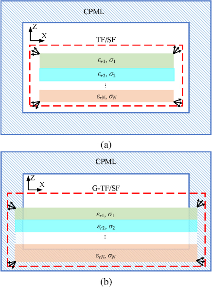
Figure 1: Conventional TF/SF and G-TF/SF boundary configuration of electromagnetic scattering from layered media: (a) conventional TF/SF and (b) G-TF/SF.
In this paper, we develop a 3D FDTD method for layered media based on the G-TF/SF technique. The new contributions of this work have two aspects. (1) The present work is the first to extend the G-TF/SF technique of the FDTD method to model 3D electromagnetic scattering from the layered media. (2) In the simulation of infinite layered media, plane waves can be introduced through CPML region. The reflected field of the medium can be obtained in the scattered field region.
II. G-TF/SF TECHNIQUE
A. Formulation of G-TF/SF technique
In this section, we derive the G-TF/SF formulation for generating plane waves in the 3D FDTD grid, with G-TF/SF boundary configured for electromagnetic scattering from layered media, as depicted in Fig. 1 (b). A discrete spatial point on a uniform rectangular lattice is denoted as . Here, , and signify incremental spacings in the , and coordinate directions, respectively, with , and as integers. Assume that the total field region is defined by , , . Note that the faces , , , and lie entirely within the CPML region, whereas a portion of the face resides within the CPML region.
Like the conventional TF/SF approach, the G-TF/SF boundary partitions the spatial lattice into two distinct regions: the total field region and the scattered field region. Therefore, the G-TF/SF approach requires that the incident field should be either subtracted or added to update equations for adjacent field nodes tangential to the boundary. In free space, the G-TF/SF algorithm is treated identically to the conventional TF/SF technique [18]. For field nodes located along the G-TF/SF boundary and situated in the CPML region, specific update equations need to be applied. We first review the standard explicit update equations for fields in the CPML region. As an illustration, the update equation for is:
| (1) |
where:
| (2) |
| (3) |
The medium-related coefficients (, ) and the CPML-related coefficients (, , and , or ) can be found in pertinent literature[18]. Here signifies the discrete time point which is an integer. The update equations for , , , and can be found in the literature [18].
Equations (A.), (A.), and (A.) hold true exclusively when all the field components () are either entirely total fields or scattering fields. Given that the field component within the G-TF/SF boundary (inclusive of the boundary itself) constitutes the total field (the sum of the incident field and the scattered field), the field component beyond the G-TF/SF boundary is the scattered field. For field nodes positioned along the G-TF/SF boundary and situated within the CPML region, the application of specific update equations is required. Let us consider the update equation for at the face of the G-TF/SF boundary within the CPML region, Equations (A.) and (A.) involve both total and scattered fields. Specifically, at and at are treated as total fields, analogous to at . However, at is treated as scattered field, rendering equations (A.) and (A.) invalid for this configuration. To derive the appropriate update equation for at the face, it is essential to incorporate the relevant incident field into equations (A.) and (A.). In other words, needs to be substituted for in equations (A.) and (A.). The formula for updating at the face is:
| (4) |
By rearranging equation (A.) in a more convenient form:
| (5) |
Similarly, the equation for updating is:
| (6) |
where and are the updated fields obtained by equations (A.) and (A.), respectively. The equation for updating is identical to equation (A.).
The remaining special update equations for the G-TF/SF boundary inside the CPML region can be derived similarly. Consequently, these equations, coupled with the conventional update equations for the TF/SF algorithm in free space, constitute the complete set of special field update equations required for the G-TF/SF method. The implementation of these special update equations is straightforward, on condition that the appropriate incident fields, such as in equations (A.) and (A.), are known. There is no need to calculate the reflected and transmitted fields.
B. Incident fields for G-TF/SF boundary
The incident electric and magnetic fields, which are essential in the convenient update equations for the G-TF/SF boundary in free space, can be acquired using a table look-up procedure [18]. For nodes adjacent to the G-TF/SF boundary in the CPML, the incident field components in the update equations necessitate a multiplicative factor, which is determined by the attenuation within the CPML.
Here, we elucidate the process to ascertain the incident electric and magnetic fields within the CPML region. These fields act as inputs to the G-TF/SF algorithm, as denoted by equations (A.) and (A.). Owing to the reflections originating from the vacuum-CPML or CPML-CPML interface, the amplitude of the electromagnetic wave does not exhibit a perfect exponential decay within CPML region. To ensure accuracy, it’s imperative to obtain the incident electric and magnetic fields within the relevant CPML region via FDTD calibration. For a specified CPML geometry, a calibration is required only once, but it is incident angle-dependent. Therefore, if the incident angle alters, an additional calibration is necessary.
Figure 2 illustrates the FDTD calibration where the measured nodes are embedded in the CPML. The TF/SF boundary has only one side, resulting in some spurious radiation from this boundary’s termination. The computational domain must be adequately large to ensure the incoming field reaches the measured nodes before this spurious radiation, thereby enabling the time-gating of the spurious radiation from the measured data. The distance between the TF/SF boundary and the CPML on the lower or upper side of the domain (Fig. 2) is unimportant — it can be as minimal as a single cell.
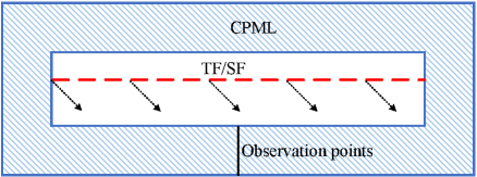
Figure 2: Geometry of preliminary CPML calibration runs used to measure attenuation of plane waves.
III. NUMERICAL RESULTS
In the succeeding illustration, if not specified, the incident wave is denoted by with the frequency of , the wavelength of . The FDTD grid consists of cubic cells with a side length of . The CPML region exhibits a thickness of . The G-TF/SF boundary in CPML extends into the CPML absorbing boundary region. A polynomial grading exponent of , and is used for the CPML implementation.
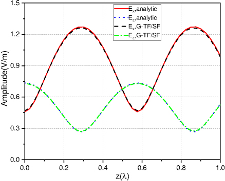
Figure 3: The amplitude of electric field at different heights above single-layer medium.
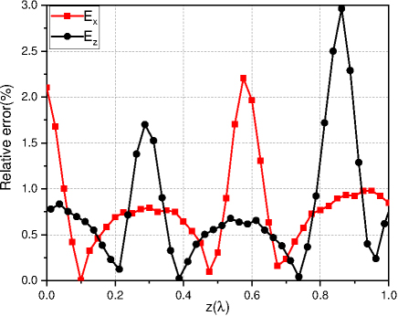
Figure 4: The relative error between G-TF/SF and the analytical method.
A. Single-layer media
We use the G-TF/SF technique to simulate the single-layer medium. The inner discrete points of CPML are , , , . Specifically, the face is treated as the interface between the free space above and the ground below, the latter being characterized by the dielectric constant and the conductivity of . The elevation and azimuthal angles of the incidence wave are , , respectively. The polarization angle is . Given that the incident wave exhibits time harmonicity, the total field environment above the medium also presents this characteristic. In this context, we solely display the amplitude of the total field above the medium.
We expect that scattering from vertices, edges, and sides, caused by the truncation of the media inside the CPML region, can be attenuated. This is attributed to the CPML region’s inherent ability to absorb electromagnetic energy. Figure 3 illustrates the amplitude of electric field components and at various heights above the single-layer lossy medium. These amplitudes are computed using both analytical and G-TF/SF methods. The analytical value is calculated by Fresnel reflection law [19]. Given that the incident wave includes a component propagating in the direction, and the reflected wave contains a component advancing in the direction, both sharing the same frequency, a stationary wave consequently materializes in the direction above the medium. Figure 4 shows the relative error between the G-TF/SF method and the theoretical method. The G-TF/SF results for the single-layer medium show good agreement with the analytical method, thereby affirming the effectiveness of the G-TF/SF method. Figure 5 presents the electric field amplitude on the face above the single-layered medium. Given the medium’s planarity, the electric field amplitude is independent of the horizontal position. The results obtained via the G-TF/SF technique adhere to physical laws.
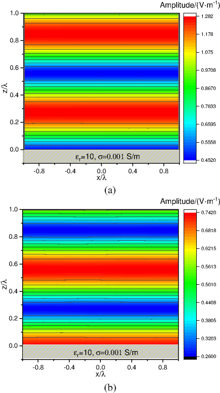
Figure 5: The electric field amplitude on face above the single-layer medium: (a) and (b) .
B. Two-layer media
The G-TF/SF technique is utilized to model a two-layered medium scenario. The inner discrete points of the CPML are , , , and . The thickness of the upper medium is quantified as a quarter-wavelength (). For the upper layer, the electrical parameters are specified as , whereas for the lower layer, they are .
Figure 6 depicts the amplitude of electric field above a two-layer medium with , and a polarization angle of , calculated by analytical [19] and G-TF/SF methods. Good agreement observed between the two methods validates the effectiveness of the G-TF/SF method. Figure 7 presents the electric field amplitude on the face above the two-layer medium. The results are computed using both conventional TF/SF and G-TF/SF methods. For the conventional TF/SF method, the associated parameters are established as follows. The region of the truncated two-layer medium is defined by , , . The conventional TF/SF boundaries are set as , , , . The interior discrete points within the CPML are denoted by , , , . Given the medium’s planarity, the electric field amplitude should be independent of the horizontal position. In the conventional TF/SF method (Fig. 7 (a)), the artificial introduction of edges and corners in the truncated layered media leads to non-physical diffraction, severely compromising the method’s accuracy. However, with the G-TF/SF method (Fig. 7 (b)), the non-physical field — originating from the CPML-embedded edges and corners of the truncated media — becomes negligible. This is because it undergoes attenuation while traversing the CPML region before it reaches the interior of the FDTD grid. The results obtained via the G-TF/SF technique adhere to physical laws.
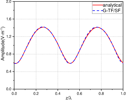
Figure 6: The amplitude of electric field at different heights above two-layer medium.
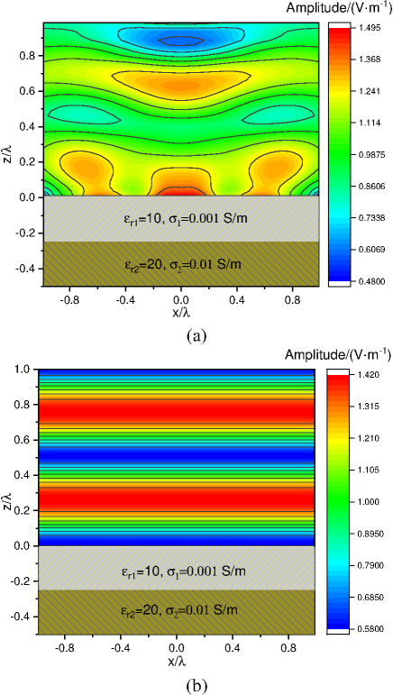
Figure 7: The electric field amplitude on face above the single-layer medium: (a) conventional TF/SF and (b) G-TF/SF.
The electrical properties of media are significant determinants of the electric field environment. Maintaining consistent electrical parameters and thickness for the upper layer ( and a thickness of ), the influence of the lower layer on the field environment is evaluated by varying the electrical parameter . Figure 8 illustrates the changes in field behaviour corresponding to different conductivities of the lower layer (), while keeping the lower layer’s dielectric constant as . In scenarios where the lower layer shares the same electrical parameters as the upper layer, specifically a conductivity of , the two layers can be regarded as a single-layer media. Figure 8 reveals that the electric field amplitude range expands with increasing bottom layer conductivity. The reason is that the increase in bottom layer conductivity elevates the reflection from the lower layer media, and subsequently, the range of electric field amplitude. The layered structure’s impact on the electric field environment is therefore non-negligible.
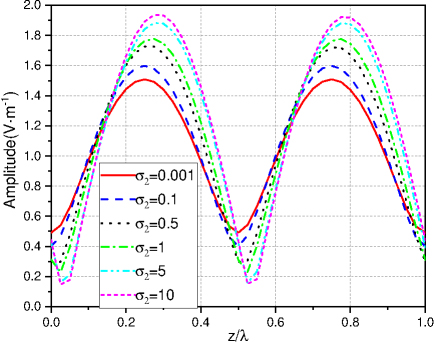
Figure 8: Sensitivity of electric field to the lower conductivity.
The influence of the upper layer’s thickness on the electric field environment is depicted in Fig. 9, assuming constant electrical parameters for both layers ( for the upper layer and for the lower one). This illustration clearly shows that the thickness of the upper layer exerts a substantial impact on the electric field environment.
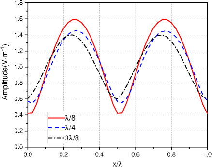
Figure 9: Sensitivity of electric field to the upper layer thickness.
Assuming that the incident plane wave is sinusoidal modulated Gaussian pulse with and . The incidence angle is and a polarization angle is . The thickness of the upper medium is . Figure 10 presents the electric field snapshot on the face at . It clearly shows the multiple reflected and transmitted waves of a layered medium.
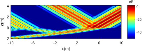
Figure 10: The absolute value of the electric field in the face.
IV. CONCLUSION
This paper presents an extension of the G-TF/SF method to the electromagnetic scattering from 3D layered media, incorporating the use of CPML ABC. The G-TF/SF method effectively mitigates the edge effects of the infinite ground in numerical simulations, thereby enhancing the precision of calculations for the layered media electromagnetic environment. The G-TF/SF method requires only the introduction of incident fields, thus circumventing the need to compute reflected and transmitted fields. Future research will explore the application of the G-TF/SF technique to layered rough media.
ACKNOWLEDGMENT
This work was supported by the National Key Research and Development Project of China under Grant 2020YFA0709800.
REFERENCES
[1] L. Lei, “An IGFBM-SAA fast algorithm for solving electromagnetic scattering from layered media rough surfaces,” Applied Computational Electromagnetics Society (ACES) Journal, vol. 39, no. 02, pp. 97–107, 2024.
[2] H. A. Sabbagh, R. K. Murphy, E. H. Sabbagh, J. C. Aldrin, J. S. Knopp, and M. P. Blodgett, “The joy of computing with volume integrals: Foundations for nondestructive evaluation of planar layered media,” Applied Computational Electromagnetics Society (ACES) Journal, vol. 25, no. 9, pp. 723–730, June 2022.
[3] L. Cao, Y. Z. Xie, and T. Liang, “An efficient FDTD-CNN method for analyzing the time-domain response of objects above layered half-space under HPEMP illumination,” IEEE Transactions on Electromagnetic Compatibility, vol. 65, no. 5, pp. 1492 – 1500, 2023.
[4] Y. Zhang, D. R. Smith, and J. J. Simpson, ‘‘A 3-D global FDTD courant-limit model of the earth for long-time-span and high-altitude applications,” Applied Computational Electromagnetics Society (ACES) Journal, vol. 39, no. 02, pp. 123–129, June 2024.
[5] X. Guo, H. Li, Y. Bo, W. Chen, L. Yang, Z. Huang, and A. Wang, “Analysis of EM properties of high-speed moving cone-sphere target coated with plasma sheath based on lorentz-FDTD method,” Applied Computational Electromagnetics Society (ACES) Journal, vol. 39, no. 02, pp. 156–168, Feb. 2024.
[6] C. Yang, X. Zhai, Z. Ren, and Z. Chen, “Analysis of electromagnetic pulse environment over irregular terrain using hybrid FDTD-GO method,” Modern Applied Physics, vol. 14, no. 1, p. 010502, 2023.
[7] P. B. Wong, G. L. Tyler, J. E. Baron, E. M. Gurrola, and R. A. Simpson, “A three-wave FDTD approach to surface scattering with applications to remote sensing of geophysical surfaces,” IEEE Transactions on Antennas and Propagation, vol. 44, no. 4, pp. 504–514, 1996.
[8] S. C. Winton, P. Kosmas, and C. M. Rappaport, “FDTD simulation of TE and TM plane waves at nonzero incidence in arbitrary layered media,” IEEE Transactions on Antennas and Propagation, vol. 53, no. 5, pp. 1721–1728, 2005.
[9] I. R. Capoglu and G. S. Smith, “A total-field/scattered-field plane-wave source for the FDTD analysis of layered media,” IEEE Transactions on Antennas and Propagation, vol. 56, no. 1, pp. 158–169, 2008.
[10] I. R. Capoglu, A. Taflove, and V. Backman, “Angora: A free software package for finite-difference time-domain electromagnetic simulation,” IEEE Antennas and Propagation Magazine, vol. 55, no. 4, pp. 80–93, 2013.
[11] Y.-N. Jiang, D.-B. Ge, and S.-J. Ding, “Analysis of TF-SF boundary for 2D-FDTD with plane p-wave propagation in layered dispersive and lossy media,” Progress in Electromagnetics Research, vol. 83, pp. 157–172, 2008.
[12] P. Chen and X. Xu, “Introduction of oblique incidence plane wave to stratified lossy dispersive media for FDTD analysis,” IEEE Transactions on Antennas and Propagation, vol. 60, no. 8, pp. 3693–3705, 2012.
[13] Y. Zhang, Y. Liu, and X. Li, “Total-field/scattered-field formulation for FDTD analysis of plane-wave propagation through cold magnetized plasma sheath,” IEEE Transactions on Antennas and Propagation, vol. 68, no. 1, pp. 377–387, 2020.
[14] Y. Zhang, N. Feng, L. Wang, Z. Guan, and Q. Liu, “An FDTD method for fully anisotropic periodic structures impinged by obliquely incident plane waves,” IEEE Transactions on Antennas and Propagation, vol. 68, no. 1, pp. 366–376, 2020.
[15] V. Anantha and A. Taflove, “Efficient modeling of infinite scatterers using a generalized total-field/scattered-field FDTD boundary partially embedded within PML,” IEEE Transactions on Antennas and Propagation, vol. 50, no. 10, pp. 1337–1349, 2002.
[16] J.-P. Berenger, “A perfectly matched layer for the absorption of electromagnetic waves,” Journal of Computational Physics, vol. 114, no. 2, pp. 185–200, 1994.
[17] J. A. Roden and S. D. Gedney, “Convolution PML (CPML): An efficient FDTD implementation of the CFS–PML for arbitrary media,” Microwave and Optical Technology Letters, vol. 27, no. 5, pp. 334–339, 2000.
[18] A. Taflove, S. C. Hagness, and M. Piket-May, Computational Electromagnetics: The Finite-Difference Time-Domain Method 3rd ed., Amsterdam, The Netherlands: Elsevier, 2005.
[19] C. A. Balanis, Balanis’ Advanced Engineering Electromagnetics. Hoboken, New Jersey: John Wiley & Sons, 2024.
BIOGRAPHIES
Chao Yang was born in Shandong Province, China, in 1991. He received the B.S. degree in Applied Physics from Xidian University, Xi’an, China, in 2014, and the Ph.D. degree in Electronic Science and Technology from Zhejiang University, Hangzhou, China, in 2019. He is currently an Assistant Research Fellow at Northwest Institute of Nuclear Technology (NINT), Xi’an, China. His research interests include computational electromagnetic, intense electromagnetic pulse environment, and electromagnetic scattering.
Haiyan Xie was born in Anhui Province, China, in 1984. She received the B.S. and Ph.D. degrees in engineering physics from Tsinghua University, Beijing, China, in 2005 and 2010, respectively. From 2011 to 2012, she conducted her postdoctoral research with the Northwest Institute of Nuclear Technology (NINT). During 2018 to 2019, she was a Visiting Scholar with the Department of Electronic Engineering, University of York, York, UK. She is currently a Professor in NINT and the Director of Research Department of Numerical Simulation of National Key Laboratory of Intense Pulsed Radiation Simulation and Effect. Her research interests mainly include electromagnetic compatibility, electromagnetic interference, and high-power electromagnetics. Xie was a recipient of the Best Doctoral Thesis of Tsinghua University in 2010 and the Young Scientist Award from the IEEE Asia-Pacific International Symposium on Electromagnetic Compatibility in 2016.
Hailiang Qiao was born in China in 1980. He received the B.S. degree in physics from Lanzhou University, Lanzhou, China, in 2003, and the M.S. degree in electromagnetic theory and microwave techniques from the Northwest Institute of Nuclear Technology (NINT), Xi’an, China, in 2011. He is currently a Research Assistant with NINT. His research interests include computational electromagnetics and plasma physics.
Xinyang Zhai was born in China in 1999. He received the B.S. degree in communication engineering from Xi’an Jiaotong University, Xi’an, China, in 2020, and the M.S. degree in nuclear science and technology from the Northwest Institute of Nuclear Technology (NINT), Xi’an, China, in 2023. He is currently working with NINT as a Research Assistant. His research interests include computational electromagnetics and electromagnetic field coupling.
Zaigao Chen was born in China in 1983. He received the B.S. degree in physical electronics from the University of Electronic Science and Technology of China in 2005, the M.S. degree in electromagnetic theory and microwave techniques from the Northwest Institute of Nuclear Technology (NINT), Xi’an, China, in 2008, and the Ph.D. degree in physical electronics from Xi’an Jiaotong University, Xi’an, China. He is currently working with NINT as an Associate Professor. His research interests mainly concentrate on numerical electromagnetic methods and plasma physics.
Yinjun Gao was born in Shaanxi Province, China, in 1983. He received the B.S. and the M.S. degree in Condensed Matter of Physics from University of Science and Technology of China, Hefei, China, in 2006 and 2009, respectively, and the Ph.D. degree in Materials Science and Engineering from Beijing Institute of Technology, Beijing, China, in 2020. He is currently an Associate Professor at Northwest Institute of Nuclear Technology (NINT), Xi’an, China. His research interests include the interaction between intense light and matter.
ACES JOURNAL, Vol. 39, No. 11, 944–951
doi: 10.13052/2024.ACES.J.391102
© 2024 River Publishers