Improving Kriging Surrogate Model for EMC Uncertainty Analysis Using LSSVR
Shenghang Huo, Yujia Song, Qing Liu, and Jinjun Bai
1College of Marine Electrical Engineering
Dalian Maritime University, Dalian 116026, China
hg1120231340@dlmu.edu.cn, liuqing@dlmu.edu.cn, baijinjun@dlmu.edu.cn
2School of Electrical Engineering
Dalian University of Technology, Dalian 116000, China
songyujia@dlut.edu.cn
Submitted On: July 21, 2024; Accepted On: September 13, 2024
ABSTRACT
As the in-depth study of uncertainty analysis in electromagnetic compatibility (EMC) progresses, the surrogate model-based uncertainty analysis method has increasingly become a popular research topic. The Kriging model is one of the classical surrogate models and plays an important role in EMC uncertainty analysis. However, an in-depth study of the Kriging sampling strategy is missing in the existing research on uncertainty analysis. The traditional sampling strategy employs Latin hypercube sampling (LHS) to select all sampling points at once, which makes the computational efficiency and accuracy of the surrogate model uncontrollable. This paper proposes a strategy that applies least squares support vector machine regression (LSSVR) to assist Kriging in sampling, significantly improving the efficiency and accuracy of the Kriging surrogate model.
Index Terms: Electromagnetic compatibility (EMC), Kriging, least squares support vector machine regression (LSSVR), surrogate model, uncertainty analysis method.
I. INTRODUCTION
In recent years, uncertainty analysis has emerged as a popular research topic in electromagnetic compatibility (EMC). By treating the input parameters in numerical simulations as uncertain parameters (e.g. random variables), the reliability and practicality of EMC simulation models can be significantly enhanced. Typically, uncertainty in simulation inputs arises from various factors, including geometric positional uncertainty due to motion or vibration, dimensional uncertainty due to manufacturing tolerances, and cognitive uncertainty due to researcher cognitive deficiencies.
The Monte Carlo method (MCM) is widely recognized as the most accurate method for uncertainty analysis [1]. It describes the randomness of the simulation inputs by exhaustively enumerating the sampling points. Because MCM considers all possible scenarios, it aligns well with the researcher’s understanding of uncertainty. Therefore, MCM is suitable for use as a standard in theoretical studies to validate the accuracy of other uncertainty analysis methods. While MCM offers the advantages of high computational accuracy and ease of implementation, its poor convergence leads to significantly low computational efficiency, rendering it less competitive in practical engineering applications [2].
In 2013, a research team at Politecnico di Torino in Italy introduced the generalized polynomial chaos (GPC) theory to EMC simulation and proposed the stochastic Galerkin method (SGM) [3]. Another numerical analysis method based on GPC theory is the stochastic collocation method (SCM) [4]. Both methods are computationally accurate and efficient. SGM is an embedded uncertainty analysis method, while SCM is a non-embedded uncertainty analysis method. With the continuous adoption of various new finite element simulation techniques in computer science, EMC design increasingly relies on commercial electromagnetic simulation software. This trend has made non-embedded simulation modes a primary focus of uncertainty analysis research in the EMC field. Consequently, the applicability of SCM exceeds that of SGM. However, SCM suffers from the serious problem of the dimensional curse of dimensionality [5] and is not applicable when dealing with a large number of random variables. The Method of Moments (MoM) [6] and the Stochastic Reduced Order Models (SROM) [7] are superior non-embedded uncertainty analysis methods for addressing the dimensional curse of dimensionality problem. However, MoM and SROM are suitable for EMC simulation solvers with good linearity. When the solver exhibits high nonlinearity, the complexity of uncertainty analysis results increases significantly, posing a risk of failure for both MoM andSROM.
Since 2020, uncertainty analysis methods based on surrogate models have been gradually proposed [8]. The principle is to treat the surrogate model as a black box and train it using deterministic simulation results repeatedly. Subsequently, a large number of samples of input randomness are taken to obtain the final results. Uncertainty analysis methods based on surrogate models can be considered as highly effective non-embedded uncertainty analysis methods. Among these, the Kriging model is a typical surrogate model used for uncertainty analysis [9,10]. It is suitable for solvers with high nonlinearity and does not encounter the issue of the dimensional curse of dimensionality. The traditional Kriging model employs a static Latin hypercube sampling (LHS) to select sampling points all at once [11], lacking the ability to actively adjust the sampling points according to specific characteristics of different situations. To enhance the accuracy and computational efficiency of the Kriging model in EMC simulation uncertainty analysis, this paper proposes an active sampling strategy that uses least squares support vector machine regression (LSSVR) to assist Kriging sampling.
The structure of this paper is as follows. Two traditional methods of uncertainty analysis, MCM and Kriging, are presented in section II. In section III, LSSVR is introduced and applied to improve the Kriging model. The improved uncertainty analysis method is applied to the parallel cable crosstalk example in section IV. Section V summarizes this paper.
II. TRADITIONAL METHODS OF UNCERTAINTY ANALYSIS
In uncertainty analysis, the random variable model is typically used to describe the uncertainty of random events:
| (1) |
where is a random variable, is a vector of random variables, and N is the number of random variables.
A. Monte Carlo method
MCM is grounded in the weak law of large numbers, which uses exhaustive sampling points to characterize a random variable , encompassing all possible cases. Where the number of sampling points is assumed to be n, and each sampling point consists of an N-dimensional vector:
| (2) |
where are all determined constant values that correspond to in equation (1).
Deterministic EMC simulation is performed at each sampling point :
| (3) |
where represents the single deterministic EMC simulation process and is the EMC simulation result. is the set of EMC simulation results, i.e., MCM-based simulation results.
The simulation results are analyzed statistically to derive uncertainty analysis results such as expectation, standard deviation, worst-case estimates, and probability density curves. Algorithm 1 shows the process of writing the code for the uncertainty analysis method based on MCM. The uncertainty analysis results of MCM are used as a reference standard in this paper.
| Algorithm 1 MCM | |
|---|---|
| 1: | Exhaustive sampling points (n) |
| 2: | for (do i=1:n) |
| 3: | EMC simulation |
| 4: | end for |
| 5: | EMC simulation result set |
| 6: | Results of uncertainty analysis |
B. Traditional Kriging model
Surrogate models significantly enhance the computational efficiency of EMC uncertainty analysis. Among these methods, the Kriging model, originating from geostatistics, is a prominent example. This section outlines the traditional Kriging-based uncertainty analysis method.
The traditional Kriging model uses LHS to select all sampling points simultaneously, with the number of sampling points denoted as L, which is significantly smaller than n. is also an N-dimensional constant value vector data. Deterministic EMC simulations are performed at each sampling point :
| (4) |
The training set is obtained, which is used to train the surrogate model. The Kriging model is an interpolation model that computes the interpolation result as a linear combination of the known sample response values:
| (5) |
where represents the weighting coefficient, and the response value at any point in the design space can be obtained by specifying the value of the weighting coefficient w. The detailed procedure for computing the weighting factor w is provided in [12]. The process of writing the code for the uncertainty analysis method based on traditional Kriging is shown in Algorithm 2.
| Algorithm 2 Traditional Kriging | |
|---|---|
| 1: | Exhaustive sampling points (n) |
| 2: | Sampling points (L) in LHS screening |
| 3: | for (do i=1:L) |
| 4: | EMC simulation |
| 5: | end for |
| 6: | Training set |
| 7: | Construction of |
| 8: | Bring into |
| 9: | Results of uncertainty analysis |
The Kriging-based uncertainty analysis method requires only deterministic EMC simulation for L samples, which is obviously much more computationally efficient than MCM.
The sampling strategy of the traditional Kriging model is to select sample points at one time by using LHS, which aims to make the sample points evenly distributed and cover the whole sampling space. However, it uses random sampling for sampling, which is a passive sampling method. It lacks the initiative to accurately select sample points that make the surrogate model more accurate. It also wastes a lot of computational resources when a single simulation takes a long time.
III. IMPROVED KRIGING BASED ON LSSVR
LSSVR is a widely used surrogate model in EMC uncertainty analysis, offering fast training speed, good generalization performance, and a strong ability to fit nonlinear functions [13]. This section presents the application of LSSVR to assist Kriging in selecting sampling points, introducing a highly proactive sequential sampling strategy that significantly enhances the accuracy and efficiency of the Kriging-based uncertainty analysis method. This combined approach is referred to as Kriging-LSSVR.
Figure 1 illustrates the structure of LSSVR, which maps the input space to a high-dimensional feature space through a nonlinear mapping . The optimal linear function is then identified in this feature space.
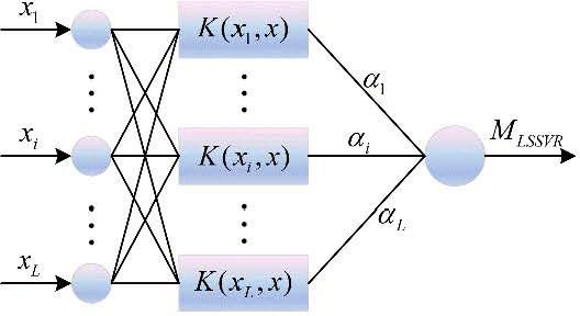
Figure 1: Structure of the LSSVR.
The dimension of the high-dimensional feature space may be infinite, and the specific expression of the nonlinear mapping is usually unknown. Thus, the kernel function technique in equation (6) is used to simplify the computation significantly by replacing the direct computation of the nonlinear mapping with the inner product of the nonlinear mapping:
| (6) |
where is the kernel function.
According to [13], LSSVR based on the Gaussian kernel function performs best in uncertainty analysis. Therefore, the Gaussian kernel function is chosen in this paper.
In this paper, LSSVR also selects sample points using LHS, and Kriging-LSSVR requires the same initial sample space for both Kriging and LSSVR. So LSSVR is trained with the training set obtained in the previous section to obtain the LSSVR model of equation (7) [14]:
| (7) |
where , are scalar coefficients, and b is the bias term.
The flowchart for applying LSSVR to improve Kriging for uncertainty analysis is shown in Fig. 2. The code writing process is described in Algorithm 3. First, the initial sample space is obtained by LHS, and it is worth noting that q is very small, even less than one-fourth of L mentioned in the previous section. The deterministic EMC simulation described in equation (3) is performed on the initial sample space to obtain the deterministic simulation result , which then produces the training set . Then, the Kriging model and the LSSVR model are constructed based on the training set. is the response value estimated by on the exhaustive sample space and is a vector of length n. is the response value estimated by .
Statistics are performed on and to obtain the probability density curves. These curves are then transformed into cumulative distribution function (CDF) curves, and the K-S distance D between the CDF curves of Kriging and LSSVR is calculated. The K-S distance is the test statistic of the Kolmogorov-Smirnov test [15]. The statistic D is determined by the maximum vertical deviation between the two curves of the CDF of the data set:
| (8) |
where is the proportion of values in the Kriging dataset that are less than or equal to x, and is the proportion of values in the LSSVR dataset that are less than or equal to x. The larger the D, the greater the difference between the two CDF curves.
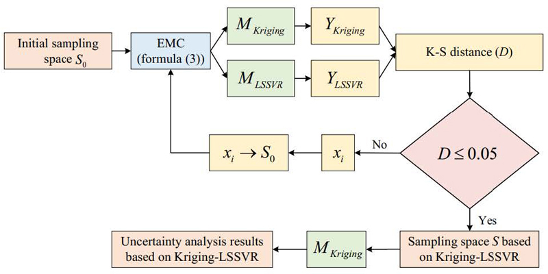
Figure 2: Flowchart of Kriging-LSSVR.
In this paper, the K-S distance D is used as a criterion to select sampling points actively. If the K-S distance exceeds 0.05, the difference between the CDF curves is considered large, indicating that the current sample space does not meet the accuracy requirements of the Kriging-LSSVR model. Find the sample point corresponding to the value with the largest difference between and , and add it to the initial sample space . The purpose of this sequential sampling strategy is to identify the point with the greatest difference between the two surrogate models, achieve uniform coverage of the sampling points in the sample space with maximum efficiency, and thereby enhance the accuracy and efficiency of the uncertainty analysis. As the sample space expands, the K-S distance D decreases. When D is less than or equal to 0.05, the final sample space is output. The EMC simulation result of sample space is the training set. The final Kriging model is constructed based on the training set. Finally, the response value is statistically analyzed to obtain the uncertainty analysis results based on Kriging-LSSVR, such as expectation, standard deviation, worst-case estimate, and probability density curve.
| Algorithm 3 Kriging-LSSVR | |
|---|---|
| 1: | Exhaustive sampling points (n) |
| 2: | LHS selects the initial sample space (q) |
| 3: | for (do i=1:q) |
| 4: | EMC simulation |
| 5: | end for |
| 6: | Initial training set |
| 7: | Construction of and |
| 8: | Bring into and |
| 9: | Statistical and |
| 10: | Generate PDF curves |
| 11: | |
| 12: | Calculate the K-S distance D |
| 13: | while do |
| 14: | Find and add it to |
| 15: | |
| 16: | Construction of and |
| 17: | Bring into and |
| 18: | Statistical and |
| 19: | Generate PDF curves |
| 20: | |
| 21: | Calculate the K-S distance D |
| 22: | end while |
| 23: | Output the final sample space |
| 24: | Determining the final Kriging model |
| 25: | Bring into |
| 26: | Results of uncertainty analysis |
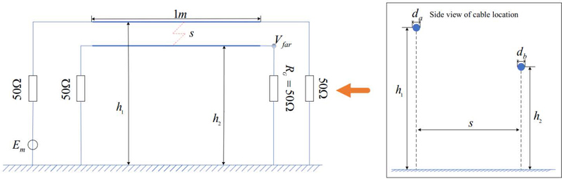
Figure 3: Parallel cable crosstalk example schematic.
IV. EXAMPLE OF APPLICATION
The Kriging-LSSVR method proposed in section III is applied to the parallel cable crosstalk example shown in Fig. 3 to verify its advantages over conventional Kriging. In practical engineering, uncertainties in cables include geometric positional uncertainties due to motion or vibration, and dimensional uncertainties due to manufacturing tolerances. Predicting crosstalk between cables considering these uncertainties is a typical EMC problem. Parallel cables are the most fundamental example of this, as discussed in [1, 16].
Two cables are parallel to each other and both have a length of 1 m. The horizontal distance between them is . One of them serves as the receptor wire and is grounded to a 50 load at each end. The other wire, the generator wire, needs to be connected not only to a 50 load, but also to an excitation source with an amplitude of 1 V. The height of the generator wire is and the diameter is . The height of the receptor wire is and the diameter is .
A. The proposed method is applied to the example with two random variables
In classical uncertainty analysis based on parallel cable crosstalk example, and are considered as two uncertain factors [1]. Here, they are assumed to follow a uniform distribution, and the results of applying random variable modeling are shown below.
| (9) |
where and are uniformly distributed random variables in the interval [-1,1].
The partial parameters of the two cables are as follows: , , .
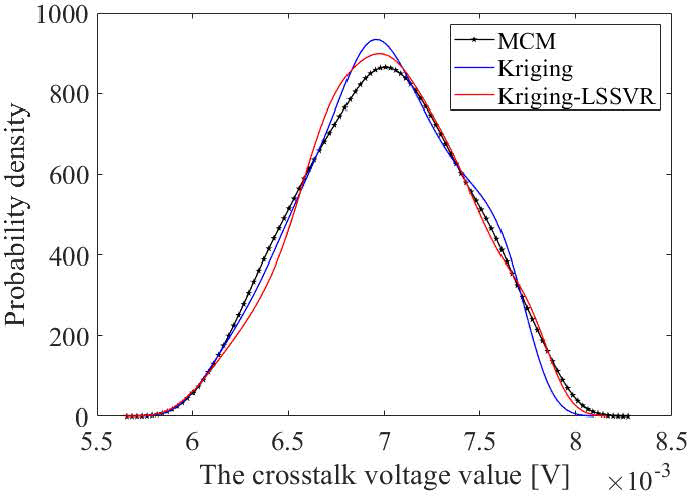
Figure 4: Probability density of crosstalk voltage values at 2 MHz.
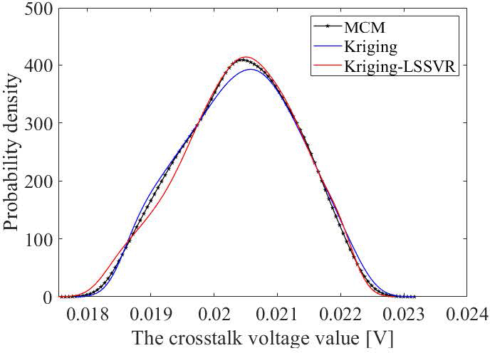
Figure 5: Probability density of crosstalk voltage values at 50 MHz.
The MCM is applied to perform 10,000 deterministic simulations at exhaustive sampling points, and the results of its uncertainty analysis are used as standard data. The initial sample space of Kriging-LSSVR has five sampling points, i.e., . The number of sampling points in the final sample space S obtained by the sequential sampling strategy is 26. In order to compare the performance of traditional Kriging and the Kriging-LSSVR proposed in this paper more objectively, the number of sampling points chosen at one time for the traditional Kriging application of LHS is also 26, i.e. . Deterministic simulation is performed on the sampling points to obtain the training set, which is used to construct the surrogate model. Subsequently, the uncertainty analysis results are obtained. Figures 4 and 5 show the probability density curves for MCM, Kriging and Kriging-LSSVR at frequencies of 2 MHz and 50 MHz, respectively.
Table 1: Results of MEAM evaluation
| Method | 2 MHz | 50 MHz |
|---|---|---|
| Kriging | 0.9573 | 0.9792 |
| Kriging-LSSVR | 0.9724 | 0.9866 |
As can be seen from the figure, the Kriging-LSSVR seems to be more accurate than Kriging, but it is not obvious. Therefore, this paper applies the mean equivalent area method (MEAM) proposed in [17] for further validation. The evaluation results of MEAM are shown in Table 1. The closer the MEAM value is to 1, the higher the accuracy of the tested method. As seen in Table 1, the accuracy of Kriging-LSSVR is higher than Kriging. However, since Kriging is already very accurate, this means the improvement in the accuracy of Kriging-LSSVR is not obvious. In order to further validate the performance of Kriging-LSSVR, the number of random variables in the parallel cable crosstalk example is expanded in this paper.
B. The proposed method is applied to the example with multiple random variables
In the parallel cable crosstalk example, in addition to the heights and of the two cables, the cable diameter and the horizontal distance between the two cables also impact the simulation results. Consider these five parameters as uniform random variables, as shown in Table 2.
Table 2: Uncertainty parameters for parallel cables
| Uniform Random Variables | Unit | U [min, max] |
|---|---|---|
| Height of generator wire | m | U [0.04, 0.05] |
| Height of receptor wire | m | U [0.03, 0.04] |
| Diameter of generator wire | mm | U [0.6, 0.8] |
| Diameter of receptor wire | mm | U [0.6, 0.8] |
| Distance between two wires | m | U [0.04, 0.06] |
MCM is applied for 10,000 simulations to obtain the standard data. Due to the increase in the number of random variables, the number of sampling points must be increased to ensure the accuracy of the surrogate model. Assume that the initial sample space of Kriging-LSSVR has 20 sampling points, i.e. . The number of sampling points in the final sample space obtained by the sequential sampling strategy is 97. The number of sampling points chosen once for the traditional Kriging application of Latin hypercube sampling is also 97, i.e. .
Figures 6 and 7 show the probability density curves at frequencies of 2 MHz and 50 MHz, respectively, and Table 3 shows the evaluation results of MEAM. As can be seen from Table 3, the accuracy of Kriging-LSSVR at 2 MHz is much higher than Kriging. The accuracy of Kriging-LSSVR at 50 MHz is also higher than Kriging, but not as much as at 2 MHz.
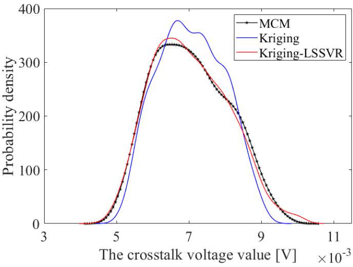
Figure 6: Probability density of crosstalk voltage values at 2 MHz.
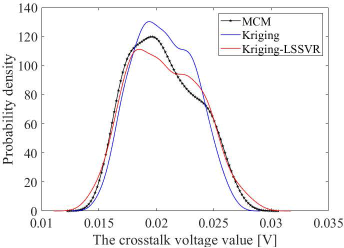
Figure 7: Probability density of crosstalk voltage values at 50 MHz.
Table 3: Results of MEAM evaluation
| Method | 2 MHz | 50 MHz |
|---|---|---|
| Kriging | 0.8678 | 0.8813 |
| Kriging-LSSVR | 0.9873 | 0.9485 |
To further investigate the performance of Kriging-LSSVR, the frequency range is extended to 1-100 MHz. As shown in Figs. 8 and 9, the expectation and standard deviation information, rather than the probability density function information, are presented. The global difference metric (GDM) values between the results to be measured and the MCM are calculated using FSV, as shown in Table 4. FSV has been successfully applied to the credibility assessment of uncertainty in EMC simulation results [1].
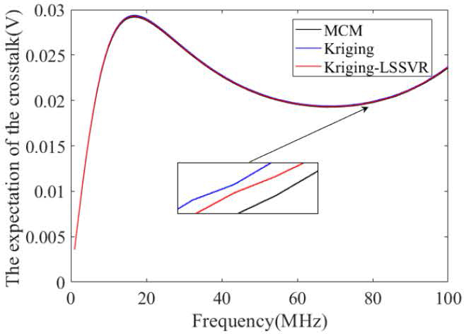
Figure 8: Far-end crosstalk voltage expectation for frequency range 1 MHz to 100 MHz.
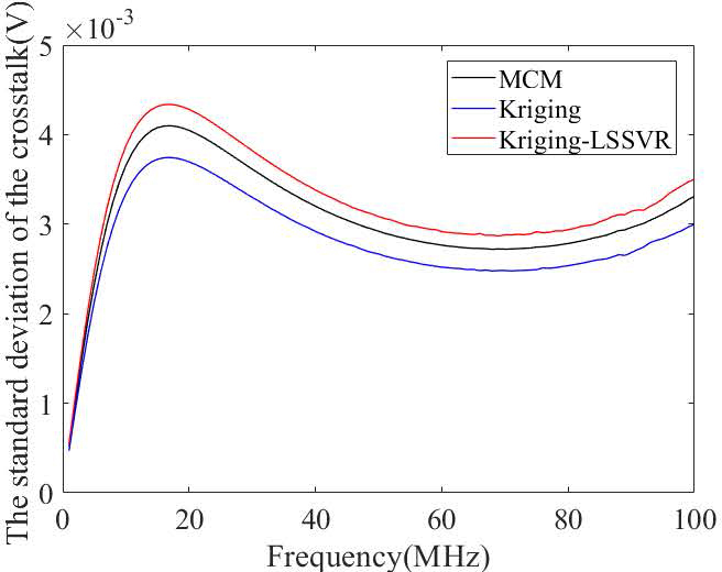
Figure 9: Standard deviation of far-end crosstalk voltage in the frequency range 1 MHz to 100 MHz.
| Kriging | Kriging-LSSVR | |
|---|---|---|
| Expectation | 0.0097 | 0.0051 |
| Standard deviation | 0.1369 | 0.0155 |
According to Table 4, the evaluation results of the expectation value of the simulation results for both surrogate models are “Excellent”. The standard deviation of Kriging is evaluated as “Very Good”, while the standard deviation of Kriging-LSSVR is rated as “Excellent”. The standard deviation evaluation result of Kriging-LSSVR is one level higher than that of Kriging, further proving that Kriging-LSSVR has higher accuracy than Kriging.
In terms of computational efficiency, it takes 28.9 seconds to perform one crosstalk computation. MCM performs a total of 10,000 simulations, taking 80 hours. Kriging and Kriging-LSSVR require only 97 computations, taking 46.7 minutes. The model prediction time of the surrogate model is negligible in comparison. The simulation time for each specific method is shown in Table 5. The model prediction time for Kriging-LSSVR is slightly longer than that of Kriging and is negligible compared to the total time . If the time for a single simulation is measured in hours, then MCM does not work. The efficiency of the surrogate model is demonstrated.
Table 5: Comparison of simulation time
| Method | |||
|---|---|---|---|
| MCM | 80 h | / | 80 h |
| Kriging | 46.7 min | 8.3 s | 46.8 min |
| Kriging-LSSVR | 46.7 min | 6.7 min | 53.4 min |
V. CONCLUSION
In this paper, LSSVR is applied to enhance the Kriging model, combining the strengths of both surrogate models to develop a more accurate and efficient EMC uncertainty analysis method, namely Kriging-LSSVR. This method enhances the proactivity of the sampling process, significantly improving the efficiency of uncertainty analysis. At high levels of simulation complexity, Kriging-LSSVR demonstrates notable advantages in accuracy and efficiency. In the parallel cable crosstalk example with multiple random variables, Kriging-LSSVR demonstrates one level higher accuracy compared to conventional Kriging. The method proposed in this paper can be applied to large-scale complex electromagnetic simulations in the future to ensure the feasibility and accuracy of large-scale simulations.
ACKNOWLEDGMENT
This paper is supported by “the Fundamental Research Funds for the Central Universities”, Project No. 3132024102.
REFERENCES
[1] J. Bai, K. Guo, J. Sun, and N. Wang, “Application of the multi-element grid in EMC uncertainty simulation,” Applied Computational Electromagnetics Society Journal, vol. 37, no. 4, pp. 428-434, Apr. 2022.
[2] R. Trinchero, M. Larbi, H. M. Torun, F. G. Canavero, and M. Swaminathan, “Machine learning and uncertainty quantification for surrogate models of integrated devices with a large number of parameters,” IEEE Access, vol. 7, pp. 4056-4066, Dec. 2019.
[3] A. Biondi, D. Vande Ginste, D. De Zutter, P. Manfredi, and F. G. Canavero, “Variability analysis of interconnects terminated by general nonlinear loads,” IEEE Trans. Compon. Packag. Manufact. Technol., vol. 3, no. 7, pp. 1244-1251, July 2013.
[4] J. Shen, H. Yang, and J. Chen, “Analysis of electrical property variations for composite medium using a stochastic collocation method,” IEEE Trans. Electromagn. Compat., vol. 54, no. 2, pp. 272-279, Apr. 2012.
[5] J. Bai, G. Zhang, A. P. Duffy, and L. Wang, “Dimension-reduced sparse grid strategy for a stochastic collocation method in EMC software,” IEEE Trans. Electromagn. Compat., vol. 60, no. 1, pp. 218-224, Feb. 2018.
[6] J. Bai, B. Hu, H. Cao, and J. Zhou, “Uncertainty analysis method for EMC simulation based on the complex number method of moments,” PIER Letters, vol. 121, pp. 7-12, 2024.
[7] Z. Fei, Y. Huang, J. Zhou, and Q. Xu, “Uncertainty quantification of crosstalk using stochastic reduced order models,” IEEE Trans. Electromagn. Compat., vol. 59, no. 1, pp. 228-239, Feb. 2017.
[8] Z. Ren, J. Ma, Y. Qi, D. Zhang, and C.-S. Koh, “Managing uncertainties of permanent magnet synchronous machine by adaptive Kriging assisted weight index Monte Carlo simulation method,” IEEE Trans. Energy Convers., vol. 35, no. 4, pp. 2162-2169, Dec. 2020.
[9] P. Besnier, F. Delaporte, and T. Houret, “Extreme values and risk analysis: EMC design approach through metamodeling,” IEEE Electromagn. Compat. Mag., vol. 10, no. 4, pp. 80-93, 2021.
[10] T. Houret, P. Besnier, S. Vauchamp, and P. Pouliguen, “Controlled stratification based on Kriging surrogate model: An algorithm for determining extreme quantiles in electromagnetic compatibility risk analysis,” IEEE Access, vol. 8, pp. 3837-3847, 2020.
[11] H. Li, B. Zhu, and J. Chen, “Optimal design of photonic band-gap structure based on Kriging surrogate model,” PIER M, vol. 52, pp. 1-8, 2016.
[12] S. Kasdorf, J. J. Harmon, and B. M. Notaroš, “Kriging methodology for uncertainty quantification in computational electromagnetics,” IEEE Open J. Antennas Propag., vol. 5, no. 2, pp. 474-486, Apr. 2024.
[13] M. Sedaghat, R. Trinchero, Z. H. Firouzeh, and F. G. Canavero, “Compressed machine learning-based inverse model for design optimization of microwave components,” IEEE Transactions on Microwave Theory and Techniques, vol. 70, no. 7, pp. 3415-3427, July 2022.
[14] S. Kushwaha, N. Soleimani, F. Treviso, R. Kumar, R. Trinchero, F. G. Canavero, S. Roy, and R. Sharma, “Comparative analysis of prior knowledge-based machine learning metamodels for modeling hybrid copper-graphene on-chip interconnects,” IEEE Trans. Electromagn. Compat., vol. 64, no. 6, pp. 2249-2260, Dec. 2022.
[15] F. J. Massey, “The Kolmogorov-Smirnov test for goodness of fit,” Journal of the American Statistical Association, vol. 46, no. 253, pp. 68-78, Mar. 1951.
[16] J. Bai, Y. Wan, M. Li, G. Zhang, and X. He, “Reduction of random variables in EMC uncertainty simulation model,” Applied Computational Electromagnetics Society Journal, vol. 37, no. 9, pp. 941-947, Sep. 2022.
[17] J. Bai, J. Sun, and N. Wang, “Convergence determination of EMC uncertainty simulation based on the improved mean equivalent area method,” Applied Computational Electromagnetics Society Journal, vol. 36, no. 11, pp. 1446-1452, Nov. 2021.
BIOGRAPHIES

Shenghang Huo received the B.Eng. degree in electrical engineering and automation from Dalian Maritime University in 2023. He is currently a graduate student in electrical engineering at Dalian Maritime University, where his research interests include machine learning and uncertainty analysis methods in EMC simulation.

Yujia Song received a Ph.D. in the School of Energy and Power Engineering at Dalian University of Technology in 2024. Her main research interests are integrated energy system design, novel power system modeling for offshore wind power, and computational electromagnetics simulation.

Qing Liu received the B.Eng. degree in electrical engineering and automation from Hubei University of Technology in 2023. He is currently a graduate student in electrical engineering at Dalian Maritime University, where his research interests include microgrid optimal dispatch, computational electromagnetics simulation for offshore wind power.

Jinjun Bai received the B.Eng. degree in electrical engineering and automation in 2013, and Ph.D. degree in electrical engineering in 2019 from the Harbin Institute of Technology, Harbin, China. He is now a lecturer at Dalian Maritime University. His research interests include uncertainty analysis methods in EMC simulation, multi-physics field simulation method.
ACES JOURNAL, Vol. 39, No. 7, 614–622
doi: 10.13052/2024.ACES.J.390705
© 2024 River Publishers