An Electromagnetic Scattering Mechanism Recognition Method Based on Deep Learning

Xiangwei Liu, Kuisong Zheng, and Jianzhou Li

School of Electronics and Information
Northwestern Polytechnical University, Xi’an Shaanxi 710072, China
xwliu@mail.nwpu.edu.cn, kszheng@nwpu.edu.cn, ljz@nwpu.edu.cn

Submitted On: July 23, 2024; Accepted On: January 28, 2025

ABSTRACT

In this paper, we proposed a data-driven deep learning (DL) method to recognize various electromagnetic (EM) scattering mechanisms. With appropriate training data containing different EM scattering mechanisms, the proposed network can accurately recognize the EM scattering mechanisms of complex models. Numerical experiments show that the DL network architecture is effective for both vertical polarization and horizontal polarization scattered field, and the average relative recognition error of the proposed method is less than 5%. This paper shows that deep neural networks have a good learning capacity for EM scattering mechanism recognition. This provides a research strategy for solving EM scattering mechanism identification in more complex EM environments.

Index Terms: Convolutional neural network, deep learning, electromagnetic scattering mechanisms, recognition.

I. INTRODUCTION

When a target is illuminated by an electromagnetic (EM) wave, the scatterer produces different scattering mechanisms, which compose the whole scattered field of the target. For example, smooth surface produces specular scattering, discontinuous structures such as edges or tips produce diffraction mechanism, and concave structures like cavities or dihedral corners induce coupling effects or multiple scattering. In addition, the whole scattered field also includes other scattering mechanisms like surface traveling waves and creep waves [1, 2].

Decomposing and recognizing different scattering mechanisms is of great significance for deep understanding and further controlling of the scattering characteristics and has a wide range of applications in radar detection such as to improve the accuracy in target recognition based on radar image. Some examples in the following section of this paper show the applicability for recognizing scattering centers, which blur the radar images, caused by edge scattering and multiplescattering.

Some high-frequency asymptotic methods, such as physical optics (PO), can produce the scattered field including only specular mechanism [3, 4]. However, the scattered field obtained by measurement or full-wave numerical methods is commonly a total radar signal, in which various scattering mechanisms are superimposed, and the specific scattering mechanism cannot be directly distinguished. Li and Liu proposed the EM scattering mechanism decomposition method based on time difference [1], which can decompose different scattering mechanisms from the whole EM scattered field. The ability to identify different scattering mechanisms is lacking with this method, which must rely on radar imaging and the experience of researchers to recognize the various components of decomposition. This experiential recognition method may not necessarily be completely accurate. Although attribute scattering center is capable of recognizing different EM scattered fields of canonical geometries, the accuracy and reliability of this method are contingent upon the models employed for the attribute scattering centers [5]. Furthermore, this approach is unable to identify the finer scattering mechanisms present in the EM scattered field.

Moreover, time frequency analysis techniques have been employed to extract scattering mechanisms. For instance, an adaptive Gaussian method was utilized to overcome the divergence of cavity scattering in radar images [6]. However, these methods either have limitations or can work only on specific scattering mechanisms. Consequently, there is currently no effective method for identifying different scattering mechanisms.

The advent of deep learning (DL) has brought us a new perspective. The method based on neural networks has performed well in many fields, such as speech recognition and image classification. Furthermore, it has found extensive and effective use in inverse scattering problems. For example, the U-Net network is utilized to learn the radar imaging mapping relationships from training data [7]. Deep neural networks are also widely used in synthetic aperture radar image classification and recognition [8, 9]. In this paper, we study the feasibility of applying DL techniques to recognize different EM scattering mechanisms. We train a deep convolutional neural network (ConvNet) to recognize different scattering mechanisms with the training data including specular scattering, multiple scattering, and edge scattering. The training dataset consists of EM scattering mechanisms calculated by various computational asymptotic electromagnetic (CAEM) methods.

This paper is organized as follows. The problem statement and methodology are presented in section II, including the CAEM methods used in this paper, the dataset used for network training, the proposed ConvNet framework, and the training results of the network. Numerical results are exhibited in section III to validate the performance of the proposed DL network. The conclusion is given in section IV.

II. METHODOLOGY

In this section, the CAEM methods used in this paper are introduced; then, the generation of our dataset used for network training, the framework, and the training results of the proposed ConvNet are demonstrated in detail.

A. CAEM methods

Various scattering mechanisms can be decomposed from the scattered field and identified through the experience of researchers [1]. This way may be used to generate a training dataset, but it requires a significant workload and may not meet the demand for training data volume.

CAEM methods can calculate the scattered field formed by different scattering mechanisms [10]. More specifically, the PO method is an algorithm that utilizes approximate integration of the induced electric field to solve the EM scattering problem [3, 4, 11]. Compared with high-precision algorithms such as the method of moments, PO does not calculate the interaction between the induced currents of different parts of the target surface, so as to solve the approximate surface-induced current independently. The scattered field calculated by PO is represented as $E_{PO}$ .

The shooting and bouncing ray (SBR) method is a high-frequency asymptotic method that combines geometrical optics (GO) and PO for solving EM scattering problems. It can obtain more accurate results by accounting for scattering caused by multiple interactions [12]. In this paper, the SBR method is employed to generate the EM scattered field containing multiple scattering. The scattered field calculated by SBR is represented as $E_{SBR}$ .

The geometrical theory of diffraction (GTD) is a generalization of GO. It is based on the exact solution of the spiked diffraction field and solves the diffraction field problem by linear correlation between the diffraction coefficients and incident field. The scattered field calculated by GTD is represented as $E_{GTD}$ .

B. Dataset generation

Training of ConvNet relies on a dataset with a large number of highly representative samples, so first, we need to generate the dataset of different scattering mechanisms. As mentioned, specular scattering, multiple scattering, and edge scattering in the training dataset can be calculated by PO, SBR, and GTD, respectively. In this paper, when calculating the target’s scattered field using the PO, SBR, and GTD algorithms, the calculation scenario assumes the far field of perfect electric conductor (PEC) targets in vacuums.

(1) Specular scattering dataset

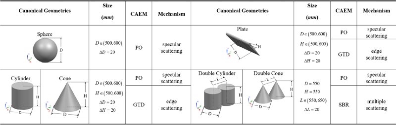
Since PO only considers specular scattering, the scattered field computed by PO can be used as part of the training dataset, as shown in equation (1). Note that specular scattering is only extracted from the scattered field of single canonical geometry, as the specular scattered field of multiple geometries can be considered as the superposition of single models. Table 1 gives the single canonical geometry model and their structural parameters:

D a t a s e t_{specular scattering} = E_{PO} .

(1)

(2) Multiple scattering dataset

Multiple scattering occurs among targets or in coupling structures, and there are too many possible ways to achieve this. Therefore, we only consider the multiple scattering generated by the coupling between canonical geometries. Table 1 shows two sets of dual models, including double cones and double cylinders, whose scattered field is calculated by PO and SBR, respectively. We can then obtain multiple scattering by equation (2). It is important to note that the scattered field calculated by SBR in this paper does not take into account edge scattering:

D a t a s e t_{multiple scattering} = E_{SBR} - E_{PO} .

(2)

(3) Edge scattering dataset

Diffraction occurs at both the edge and the tip but, due to very rapid attenuation of EM scattering at the tip, it is usually ignored. Therefore, in this paper only edge scattering is considered. GTD and PO are used to calculate the scattered field of canonical geometries with edge in Table 1. Then we obtain the contribution of the edge to the scattered field by equation (3):

D a t a s e t_{edg scattering} = E_{GTD} - E_{PO} .

(3)

To demonstrate the accuracy and reliability of the data generation method, we use it to process the scattered field of models with coupled structures. The double PEC sphere model is illustrated in Fig. 1, wherein the spheres exhibit a strong coupling effect when in close proximity.

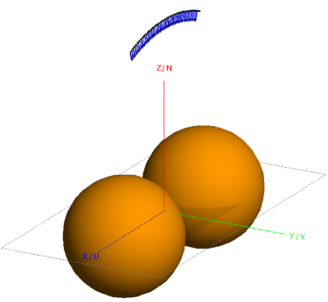
Figure 1: Double PEC spheres. The diameter of both spheres is $300 m m$ , and the interval between them is $100 m m$ .

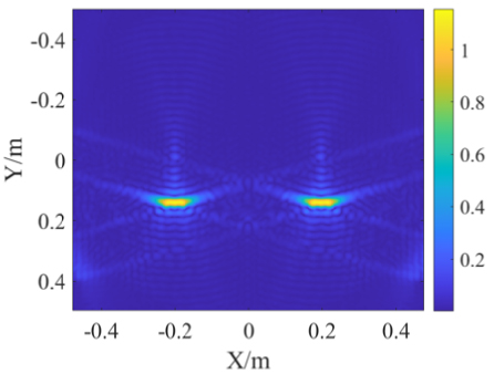
Figure 2: Radar image of the double PEC spheres by PO.

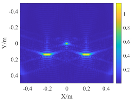
Figure 3: Radar image of the double PEC spheres by SBR.

Table 1: Dataset components

The scattered field of the double PEC spheres is calculated by PO and SBR, respectively. The direction of incidence wave is from $θ = - 20^{\circ} φ = 0^{\circ}$ to $θ = 20^{\circ} φ = 0^{\circ}$ with $1^{\circ}$ interval. The frequency is taken to be from 6 GHz to 12 GHz, with 0.15 GHz interval. Their corresponding radar images are shown in Figs. 2 and 3, respectively. The y-range resolution and x-range resolution of the radar imaging are 0.025m and 0.0239m, respectively. In this paper, $θ$ represents the angle between the incident wave and the z-axis, while $φ$ denotes the angle between the projection of the incident wave onto the xoy-plane and the x-axis. The radar imaging algorithm used in this paper is the backward propagation algorithm [13]. As illustrated in Fig. 2, only two scattering centers are evident. It can be observed that these correspond to the specular scattering from the two spheres. However, Fig. 3 demonstrates a pronounced presence of an extra scattering center at point (0, 0), indicating a strong coupling between the two spheres. It is evident that this discrepancy is caused by the strong multiple scattering mechanism. In the absence of knowledge regarding the number of metal spheres, it is possible to ascertain that the model comprises three metal spheres based on the scattering center observed in Fig. 3. However, this conclusion is not aligned with the actual structural composition of the target. Furthermore, this example highlights the significance of recognizing different scattering mechanisms. Subsequently, equation (2) is employed to process the scattered field of the double PEC spheres. Thereby we can get the multiple scattering, as illustrated in the radar image of Fig. 4. A comparison of Figs. 4 and 3 reveals that multiple scattering has been accurately extracted from the scattered field computed by SBR. The coupling mechanism between the targets is strongly influenced by the distance between them. As a result, when the distance between the targets is large, the coupling effect weakens, and they do not form a prominent scattering center in the radar image. To observe significant coupling fields in the radar image, it is crucial to carefully determine the optimal distance between the targets.

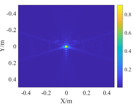
Figure 4: Radar image of multiple scattering of the double PEC spheres.

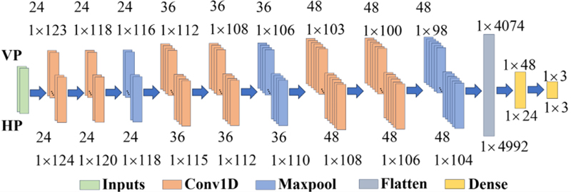
Figure 5: ConvNet architecture.

As shown in Table 1, the selected CAEM methods calculate the scattered field of different geometries, and both vertical polarization (VP) and horizontal polarization (HP) are considered. The direction of incidence wave is from $θ = 0^{\circ}, φ = 0^{\circ}$ to $θ = 90^{\circ}, φ = 0^{\circ}$ with $θ = {0.5}^{\circ}$ interval, and the frequency is from 6 GHz to 18 GHz. The number of samples is 128. The training dataset consists of scattering mechanisms at different incident angles, represented as complex numbers with varying dimensions depending on the calculation frequency. Both VP and HP datasets contain approximately 15,000 scattering mechanisms, with 12,000 used for training and 3,000 for testing.

C. ConvNet

In theory, neural networks can approximate any continuous function. In this work, we employ ConvNet as the DL method. ConvNet architecture is shown in Fig. 5. It consists of six convolutional layers, which are responsible for feature extraction. These layers apply a range of filters to the input, detecting low-level features in the early layers and higher-level features as the network deepens. To reduce the number of parameters and retain useful features, three max-pooling layers are inserted between the convolutional layers. This also helps prevent overfitting by making the model more invariant to small translations in the input data. After the convolutional and pooling layers, a flattening layer is used to convert the multi-dimensional output into a one-dimensional vector. This step is essential for linking the convolutional part of the network to the fully connected layers, enabling the network to perform classification based on the extracted features. The network includes two fully connected layers that follow the flattening layer. These layers are responsible for the final classification task, mapping the flattened features to output class probabilities using learned weights. The first fully connected layer processes the feature vector, while the second produces the final class predictions.

The rectified linear unit (ReLU) activation function is applied in the convolutional layers to introduce non-linearity, allowing the network to learn more complex patterns. ReLU also mitigates the vanishing gradient problem, which can occur with other activation functions. In the fully connected layers, the SoftMax activation function is used to convert the network’s output into probability distributions, ensuring that the final output is interpretable as class probabilities.

The input to ConvNet consists of two 1 $\times$ 128 vectors, representing the real and imaginary parts of the scattering mechanisms. These vectors serve as features for the network to learn patterns for classification. The real and imaginary components are essential for capturing the complex nature of the scattering data, allowing the network to learn both magnitude and phase information. As shown in Fig. 5, ConvNet architecture is effective for both HP and VP, although the kernel sizes differ. The optimization algorithm used in ConvNet is the adaptive moment estimation (ADAM) algorithm [14], an efficient method for stochastic gradient-based optimization.

Moreover, the cross-entropy loss function widely used in multi-classification problems is adopted in ConvNet, as shown in equation (4):

L o s s = - \sum_{i = 1}^{N} y_{i} ∙ \log {\hat{y}}_{i},

(4)

where $y_{i}$ and ${\hat{y}}_{i}$ represent the true labels and predicted labels, respectively, and $N$ is the number of categories.

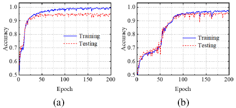
Figure 6: Training and testing performance of ConvNet: (a) and (b) are the accuracy curves of the VP dataset and HP dataset, respectively.

Variations in accuracy during training and testing epochs are shown in Fig. 6. It is evident that the accuracy of training is better than that of testing when the model is convergent. The training and testing accuracy curves in Fig. 6 (a) converge to 0.98 and 0.95 after 100 and 50 iterations, respectively. Similarly, the training and testing accuracy curves in Fig. 6 (b) converge to 0.96 and 0.95, respectively, after 100 iterations. The hardware configuration includes an Intel 13th i9 CPU running at 3 GHz with 128 GB memory. The entire dataset requires a training time of 10 minutes and utilizes 20 GB of memory for the training process.

The confusion matrix in Fig. 7 illustrates three distinct scattering mechanisms, labeled as 1 (specular scattering), 2 (edge scattering), and 3 (multiple scattering). It can be seen from Fig. 7 that the overall classification accuracy is above 95% and the individual classification accuracy is above 93% for all different scattering mechanisms. As can be observed in Table 1, the sources of specular scattering are particularly diverse. In contrast, the sources of multiple scattering and edge scattering are relatively limited, which makes specular scattering more challenging to recognize. Consequently, the network’s recognition of specular scattering is somewhat lower compared to the other two. Nonetheless, the above results indicate that the proposed ConvNet has the ability to accurately identify different scattering mechanisms. To verify the robustness and generalization ability of ConvNet, in section III we use ConvNet to recognize the scattering mechanism of two scatters not inTable 1.

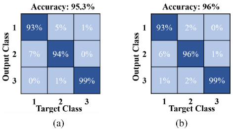
Figure 7: Confusion matrix based on ConvNet: (a) and (b) are the recognition results of VP and HP test sets, respectively. 1 $=$ specular scattering, 2=edge scattering, and 3 $=$ multiple scattering.

III. NUMERICAL RESULTS

In this section, the proposed ConvNet is employed to recognize different scattering mechanisms under more complex conditions. The initial step is to identify the scattering mechanism of a combinatorial model that is not included in Table 1. Subsequently, the scattering mechanism of a complex model formed by canonical geometries in Table 1 is identified. The effectiveness of the proposed method can be demonstrated through these arithmetic examples.

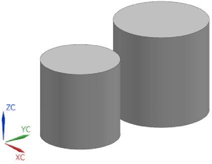
Figure 8: Coupled scatter.

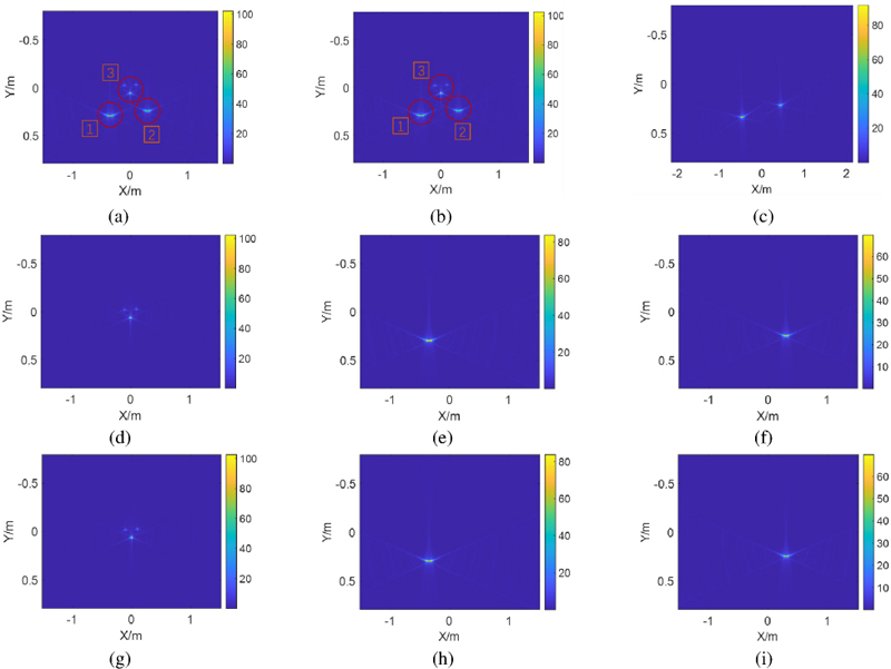
Figure 9: Radar images of coupled scatters: (a) and (b) are radar images calculated by SBR for VP and HP, respectively, (c) is the radar image calculated by PO, (d-f) are radar images of the decomposition of VP scattered field, and (g-i) are radar images of the decomposition of the HP scattered field.

A. Coupled scatter

Coupled scatter comprise two cylinders of different sizes as illustrated in Fig. 8: one with a diameter and height of $600 m m$ and the other with a diameter and height of $500 m m$ , separated by a distance of $100 m m$ .

The scattered field of the coupled scatter is calculated by SBR, with the incident wave frequency ranging from 6 GHz to 18 GHz and the VP and HP incident wave angles ranging from $θ = 90^{\circ}, φ = - 15^{\circ}$ to $θ = 90^{\circ}, φ = 15^{\circ}$ . There are 128 sampling points for both frequency and angle. The y-range resolution and x-range resolution of the radar imaging are 0.0125m and 0.0239m, respectively.

The radar images for VP and HP are illustrated in Figs. 9 (a) and (b), respectively, which show multiple scattering centers between the two cylinders. In order to assist in the depiction of the scattering centers in Figs. 9 (a) and (b), we have labelled the different scattering centers. Figure 9 (c) shows the radar image of the coupled scatter calculated by PO, and its comparison with Figs. 9 (a) and (b) indicates that multiple scattering between cylinders have formed strong scattering centers 333, which could interfere with radar recognition.

We use the decomposition algorithm [1] to decompose different scattering components from the row scattered field of the coupled scatters. Alternatively, methods such as CLEAN can be employed to extract scattering centers from radar images [15], and the corresponding scattering data can be inverted using these extractedcenters.

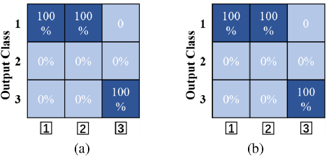
Figure 10: Confusion matrix of coupled scatter: (a) and (b) are the recognition results of the scattering mechanisms decomposed from VP and HP scattered field of the coupled scatter, respectively.

The decomposition results of VP and HP scattered field of the coupled scatters are shown in Figs. 9 (d-i). ConvNet recognition results of the decomposed scattering components are shown in Fig. 10. It is evident from the confusion matrix in Fig. 10 that the decomposed scattering mechanisms corresponding to 313 and 323 have been identified as specular scattering and the decomposed scattering mechanism corresponding to 333 has been identified as multiple scattering mechanism, which is consistent with our analysis. It should be noted that there is no edge scattering in the scattered field of the coupled scatter, so the second row in confusion matrix is 0.

B. Complex scatter

Complex scatter is composed of canonical geometries, including two sets of wings, a hemisphere, an ellipsoid, and a cylinder as shown in Fig. 11. The dimensions of the complex scatter are shown in Table 2. The angle between the axis of the complex scatter and the xoz-plane is 40 $^{\circ}$ . The scattered field of the complex scatter is calculated by GTD and PO, respectively, with the incident wave frequency ranging from 6 GHz to 18 GHz and the VP and HP incident wave angles ranging from $θ = 90^{\circ}, φ = - 15^{\circ}$ to $θ = 90^{\circ}, φ = 15^{\circ}$ . There are 128 sampling points for both frequency and angle. The y-range resolution and x-range resolution of the radar imaging are 0.0125m and 0.0239m, respectively.

Radar images of the scattered field calculated by GTD are shown in Figs. 12 (a) and (b). In order to assist in the depiction of the scattering centers in Fig. 12, we have labelled the different scattering centers. Figs. 12 (a) and (b) both exhibit a point scattering center $1⃝$ . However, there are three pairs of sheet scattering centers in Fig. 12 (a) for VP, but four such pairs in Fig. 12 (b) for HP. By comparing the radar image of the PO-calculated scattered field as shown in Figs. 12 (c) and Figs. 12 (a) and (b), it can be seen that the additional slab scattering centers in Figs. 12 (a) and (b) are obviously caused by edge scattering.

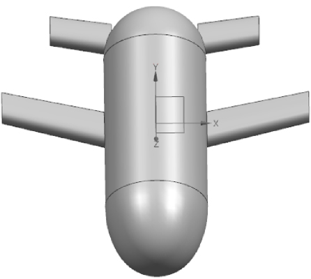
Figure 11: Complex scatter.

Table 2: Dimensions of complex scatter

L: Length, W: Width, T: Thickness, D: Diameter (mm)
Long Wings	Short Wings	Hemisphere	Ellipsoid	Cylinder
L: 521, W: 178, T: 51	L: 308, W: 166, T: 50	D: 508	D: 508, L: 371	D: 508, L: 840

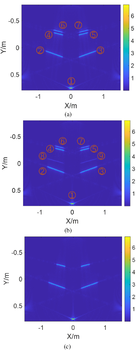
Figure 12: Radar images of the complex scatter: (a) and (b) are radar images calculated by GTD for VP and HP, respectively, and (c) is the radar image calculated by PO.

The scattered field of the complex scatter is decomposed to obtain the scattering contributions corresponding to different scattering centers, and we then use the trained ConvNet to recognize which scattering mechanism they belong to. The classification recognition results of different scattering contributions are shown in Fig. 13.

In Fig. 13 (a), $1⃝$ , $4⃝$ , and $5⃝$ are identified as specular scattering, with a recognition rate of over 90%. $6⃝$ and $7⃝$ are identified as edge scattering with a recognition rate of about 90%. These recognition errors may be caused by the occlusion between structures. Because the edge scattering and specular scattering of the complex scatter’s long wings for VP jointly form $2⃝$ and $3⃝$ , ConvNet cannot accurately recognize $2⃝$ and $3⃝$ . In Fig. 13 (b), the scattering mechanisms corresponding to each scattering center have been effectively identified, with a recognition probability of no less than 86%. $1⃝$ , $2⃝$ , $3⃝$ , $4⃝$ , and $5⃝$ are identified as specular scattering mechanisms by the trained ConvNet, and $6⃝$ and $7⃝$ are identified as edge scattering with a recognition rate of about 90%.

There are two additional scattering centers $8⃝$ and $9⃝$ in Fig. 13 (b), which are identified as edge scattering. This is due to the fact that the polarization characteristics of the incident wave exert a considerable influence on the edge scattering. In the HP case, a pair of slice scattering centers is created in the radar image, which significantly increases the probability of $2⃝$ and $3⃝$ being identified as specular scattering compared to Fig. 13 (a).

It is worth noting that, for complex scatter, the combination of canonical geometries results in a change in their scattered field compared to that generated solely by themselves. Therefore, although the recognition rate of ConvNet for the scattering mechanism of complex scatter is lower than that of the training dataset, the recognition results in this paper have fully demonstrated the effectiveness and generalization ability of the proposed ConvNet.

Moreover, this paper validates the capacity of ConvNet to recognize different scattering mechanisms. Nevertheless, due to the restricted quantity of data in the dataset and the limited number of model types considered, we have not yet validated the network’s capacity to identify scattering mechanisms for more complex models. However, we are gradually augmenting the dataset with additional corresponding samples, which will allow us to assess the network’s performance. This is a promising avenue for further investigation.

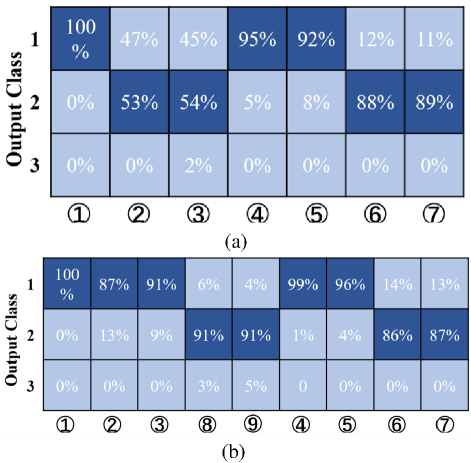
Figure 13: Confusion matrix of the complex scatter: (a) and (b) are the identification results of the scattering mechanisms decomposed from VP and HP scattered field, respectively.

IV. CONCLUSION

This paper proposes a DL-based method for recognizing scattering mechanisms, which demonstrates high accuracy and robust generalization through numerical experiments. Results show that the method significantly improves the identification of scattering mechanisms, offering a reliable alternative to traditional experience-based techniques. In particular, the method accurately classifies different scattering centers in radar images, even under challenging conditions. Moreover, the proposed method exhibits strong potential for broader applications in radar imaging. For example, expanding its use to scenarios such as traveling wave recognition could further enhance both the precision and range of scattering mechanism identification by incorporating a wider variety of targets. The method’s ability to generalize across different scenarios highlights its versatility, and future work will focus on exploring additional use cases to further optimize its performance andapplicability.

REFERENCES

[1] J. Li and X. Liu, “A method of decomposition and extraction of scattering mechanisms based on time slot difference,” IEEE Transactions on Antennas and Propagation, vol. 69, no. 3, pp. 1560-1568, Mar. 2021.

[2] X. Liu, J. Li, Y. Zhu, and S. Zhang, “Scattering characteristic extraction and recovery for multiple targets based on time frequency analysis,” Applied Computational Electromagnetics Society (ACES) Journal, vol. 35, no. 8, pp. 962-970, Aug. 2020.

[3] W. Gordon, “Far-field approximations to the Kirchoff-Helmholtz representations of scattered fields,” IEEE Transactions on Antennas and Propagation, vol. 23, no. 4, pp. 590-592, July1975.

[4] M. Kara and M. Mutlu, “Scattering and diffraction evaluated by physical optics surface current on a truncated cylindrical conductive cap,” Applied Computational Electromagnetics Society (ACES) Journal, vol. 38, no. 05, pp. 304-308, May2023.

[5] H. Liu, B. Jiu, F. Li, and Y. Wang, “Attributed scattering center extraction algorithm based on sparse representation with dictionary refinement,” IEEE Transactions on Antennas and Propagation, vol. 65, no. 5, pp. 2604-2614, May2017.

[6] X.-Y. He, G.-D. Tong, W. Gao, X.-L. Mi, P.-C. Gao, and Y. Zhang, “The method of adaptive Gaussian decomposition-based recognition and extraction of scattering mechanisms,” in 2018 12th International Symposium on Antennas, Propagation and EM Theory (ISAPE), Hangzhou, China, pp. 1-4, 2018.

[7] Z. Wei and X. Chen, “Deep-learning schemes for full-wave nonlinear inverse scattering problems,” IEEE Transactions on Geoscience and Remote Sensing, vol. 57, no. 4, pp. 1849-1860, Apr.2019.

[8] D. He, W. Guo, T. Zhang, Z. Zhang, and W. Yu, “Occluded target recognition in SAR imagery with scattering excitation learning and channel dropout,” IEEE Geoscience and Remote Sensing Articles, vol. 20, pp. 1-5, 2023.

[9] N. Kussul, M. Lavreniuk, S. Skakun, and A. Shelestov, “Deep learning classification of land cover and crop types using remote sensing data,” IEEE Geoscience and Remote Sensing Articles, vol. 14, no. 5, pp. 778-782, May 2017.

[10] F. A. Molinet, “Modern high frequency techniques for RCS computation: A comparative analysis,” Applied Computational Electromagnetics Society (ACES) Journal, vol. 6, no. 1, pp. 31-58, July2022.

[11] J. Perez and M. F. Catedra, “Application of physical optics to the RCS computation of bodies modeled with NURBS surfaces,” IEEE Transactions on Antennas and Propagation, vol. 42, no. 10, pp. 1404-1411, Oct. 1994.

[12] H. Ling, R.-C. Chou, and S.-W. Lee, “Shooting and bouncing rays: Calculating the RCS of an arbitrarily shaped cavity,” IEEE Transactions on Antennas and Propagation, vol. 37, no. 2, pp. 194-205, Feb. 1989.

[13] M. D. Desai and W. K. Jenkins, “Convolution back projection image reconstruction for spotlight mode synthetic aperture radar,” IEEE Transactions on Image Processing, vol. 1, no. 4, pp. 505-517, Oct. 1992.

[14] D. P. Kingma and J. Ba, ADAM: A Method for Stochastic Optimization [Online]. Available: https://arxiv.org/abs/1412.6980

[15] M. Martorella, N. Acito, and F. Berizzi, “Statistical CLEAN technique for ISAR imaging,” IEEE Transactions on Geoscience and Remote Sensing, vol. 45, no. 11, pp. 3552-3560, Nov.2007.

BIOGRAPHIES

Xiangwei Liu is currently pursuing his Ph.D. at Northwestern Polytechnical University. His current research interests include electromagnetic signal analysis and intelligent electromagnetic simulation calculation.

Kuisong Zheng is an associate professor at Northwestern Polytechnical University. He received his Ph.D. from Xidian University in 2006. From 2006 to 2008, he was a postdoctoral researcher at the Hong Kong Polytechnic University. His research interests include electromagnetic modeling and simulation.

Jianzhou Li is an associate professor at Northwestern Polytechnical University. He received his Ph.D. degree in 2005 from Northwestern Polytechnical University. He was a postdoctoral researcher at University of Surrey, UK, 2008-2009. His research interests focus on electromagnetic modeling and simulation.