Superior Accuracy of the Normally-integrated MFIE Compared to the Traditional MFIE

Andrew F. Peterson and Malcolm M. Bibby

School of Electrical and Computer Engineering
Georgia Institute of Technology, Atlanta, GA 30332-0250, USA
peterson@ece.gatech.edu, mbibby@ece.gatech.edu

Submitted On: July 23, 2024; Accepted On: March 31, 2025

ABSTRACT

An alternative method of moments discretization of the magnetic field integral equation (MFIE) uses testing functions inside the target and in a plane normal to the target surface. This approach is adapted to targets modeled with flat-faceted patches. A comparison with traditional numerical solutions of the MFIE that use testing functions on the target surface shows that the normally-integrated MFIE formulation produce far fields that are more accurate than those obtained from the traditional MFIE. The alternate approach can be made free from internal resonances and that approach is often more accurate than the combined field integral equation.

Index Terms: Electromagnetic scattering, method of moments, numerical techniques, radar cross section, scattering cross section.

I. INTRODUCTION

Integral equations such as the electric-field equation (EFIE) and magnetic field integral equation (MFIE) are the foundation for many numerical solution techniques in electromagnetics, especially open-region problems such as radiation and scattering applications involving perfectly conducting materials. The most common discretization procedure used with the EFIE involves Rao-Wilton-Glisson (RWG) basis and testing functions [1], which converts the “strong” form of the EFIE into a “weak” equation where the degree of the operator derivative has been reduced by the testing function. A similar discretization of the MFIE does not produce a “weak” equation since one of the MFIE derivatives is normal to the surface being discretized and not affected by the tangential testing function. The MFIE has other restrictions: it is not applicable to open targets and may fail under certain conditions for multiply connected targets [2]. Both equations many fail at internal resonance frequencies [3]. In addition, the MFIE is thought to be more sensitive to discontinuities, such as those introduced by flat-faceted models of curved surfaces [4].

The accuracy of the far fields (and scattering cross section) produced by traditional MFIE discretizations is substantially worse than that produced by the EFIE [5–6]. When the EFIE and MFIE are combined together to form the combined field integral equation (CFIE) to avoid internal resonance failures, the accuracy of the CFIE is degraded by the underlying MFIE accuracy and seldom equals that of the EFIE away from resonances.

In [7–8], an alternative discretization was introduced for the MFIE, involving testing functions that are inside the target and in a plane normal to the surface. These functions can absorb both derivatives arising from the curl operator. The approach, labeled the normally-integrated MFIE or NIMFIE, produces a true “weak” equation different from that of the traditional tangentially-tested MFIE. In [7–9], the NIMFIE was demonstrated for several smooth targets, using high order basis functions and perfect models of the curved target surfaces. In order to employ the NIMFIE for more complex targets modeled with flat patch models, a new discretization is proposed with RWG basis functions representing the current and testing functions with support that may be divided into two non-overlapping domains inside the target. Results from the new approach will be compared with those produced by a conventional MFIE discretization (also using RWG basis functions but with RWG testing functions located on the target surface). In addition, [8] demonstrated that, by including an exponential phase in the testing functions, the original NIMFIE equations could be made free of internal resonances. Consequently, we use the “resonant free” approach in the following and also compare the results to those of the CFIE. Preliminary results from this study were presented in [10–11].

II. NIMFIE FORMULATION

The NIMFIE formulation is based on the condition that the total magnetic field vanishes inside a perfectly conducting target. Therefore, the incident and scattered magnetic fields satisfy:

$$\overline{T}\bullet {\overline{H}}^{inc}+\overline{T}\bullet {\overline{H}}^s=0,$$

(1)

where the incident field is that of the primary source in the absence of the target, and the scattered field is the field of the equivalent current density $\overline{J}$ on the target surface, also computed in the absence of the target. The testing function $\overline{T}$ occupies a plane normal to the surface of the target and is a vector perpendicular to that plane. The scattered field is obtained from:

$${\overline{H}}^s=\nabla \times \overline{A},$$

(2)

where $\overline{A}$ is the magnetic vector potential function:

$$\overline{A}(\overline{r})=\int \int \overline{J}(s^{\prime },t^{\prime })\frac{e^{-jkR}}{4\pi R}d{s}^{\prime }d{t}^{\prime }.$$

(3)

The integral in (3) is over the target surface, $k=\omega \sqrt{{\mu }_0{\epsilon }_0}$ is the wavenumber of the background medium, $\omega$ is the radian frequency, and ${\mu }_0$ and ${\epsilon }_0$ are the permeability and permittivity of the background medium. The parameter R is the distance from the point of integration to the point where the field is computed.

For targets represented by flat-faceted triangular patches, the basis functions representing the current density are chosen to be RWG functions that straddle pairs of patches and interpolate to the current density flowing across edges of the model [1]. For convenience each testing function will also be associated with an edge. The test function domain associated with two patches straddling an edge p is inside the target, beginning below the centroid of one patch (A) and terminating beneath the centroid of an adjacent patch (B), as depicted in Fig. 1. For patch pairs that are bent to represent curved or non-planar parts of surfaces, the testing domain in the present work is separated into two non-overlapping rectangular regions as depicted in the side view shown in Fig. 1 (b). Let (s, t, n) denote a local right-handed coordinate system associated with a patch, with variables s and t tangential to the patch and n in the outward normal direction. In the “internal resonance free” NIMFIE formulation, the part of the test function below one of the two patches is:

$$\overline{T}=\widehat{s}p(t;t1,t2)e^{-j\phi (n2-n)}p(n;n1,n2),$$

(4)

where p(t;t1,t2) denotes a windowing function:

$$p(t;t1,t2)=\{\begin{array}{cc}\hfill 1\hfill & \hfill t1<t<t2\hfill \\ \hfill 0\hfill & \hfill otherwise\hfill \end{array},$$

(5)

and the rectangular domain is the region t1$<$t$\mathrm{<}$t2, n1$<$n$\mathrm{<}$n2. The phase factor:

$$\phi =\frac{\pi }{2}\frac{1}{n2-n1},$$

(6)

provides a 90-degree phase progression across the test function domain, to suppress internal resonances in a manner similar to that of the dual surface integral equations [12].

The NIMFIE equation associated with the complete contribution from the basis function associated with edge q and the two parts of the test function associated with edge p can be obtained by inserting (4) and its complement into the relation:

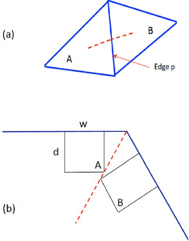
Figure 1: (a) Top and (b) side views of a patch pair showing the two parts of the domain of the testing function when the patches are non-planar.

$$-\int \int \overline{T}\bullet {\overline{H}}^{inc}=\int \int \overline{T}\bullet \nabla \times \overline{A},$$

(7)

where the integrations are over the test domain inside the target. By carrying out any integrations that cancel derivatives arising from the curl operation, we obtain the resulting equation:

$$\begin{array}{cc}& -{\int }_{n1A}^{n2A}{\int }_{t1A}^{t2A}{e}^{-j\phi (n2A-n)}{\widehat{s}}_{pA}\bullet {\overline{H}}^{inc}\hfill \\ & -{\int }_{n1B}^{n2B}{\int }_{t1B}^{t2B}{e}^{-j\phi (n2B-n)}{\widehat{s}}_{pB}\bullet {\overline{H}}^{inc}\hfill \\ & ={{\int }_{n1A}^{n2A}{e}^{-j\phi (n2A-n)}{\widehat{n}}_{pA}\bullet \overline{A}|}_{t1A}^{t2A}\hfill \\ & +{{\int }_{n1B}^{n2B}{e}^{-j\phi (n2B-n)}{\widehat{n}}_{pB}\bullet \overline{A}|}_{t1B}^{t2B}\hfill \\ & -{{\int }_{t1A}^{t2A}\left(e^{-j\phi (n2A-n)}{\widehat{t}}_{pA}\bullet \overline{A}\right)|}_{n1A}^{n2A}\hfill \\ & -{{\int }_{t1B}^{t2B}\left(e^{-j\phi (n2B-n)}{\widehat{t}}_{pB}\bullet \overline{A}\right)|}_{n1B}^{n2B}\hfill \\ & +j{\phi }_A{\int }_{n1A}^{n2A}{\int }_{t1A}^{t2A}{e}^{-j\phi (n2A-n)}{\widehat{t}}_{pA}\bullet \overline{A}\hfill \\ & +j{\phi }_B{\int }_{n1B}^{n2B}{\int }_{t1B}^{t2B}{e}^{-j\phi (n2B-n)}{\widehat{t}}_{pB}\bullet \overline{A}\hfill \end{array},$$

(8)

where the integration limits such as “t1A” are those associated with the part of the test domain under patch “A” and limits such as “t1B” are those associated with the test domain under patch “B” (Fig. 1). Similarly, unit vectors exhibit an “A” or “B” subscript to denote which test patch (A or B) they are associated with. Equation (8) is slightly different from those in [8] due to the vector nature of the RWG basis and the two distinct domains associated with the testing function.

Observe that there are no derivatives applied to the magnetic vector potential function in (8), confirming that this orientation of the test function absorbs all the derivatives arising from the curl operation and produces a truly “weak” form of the integral equation. For numerical implementation, the integrals in (8) are no more difficult to compute than those arising from the traditional EFIE discretizations.

Ideally, to suppress internal resonances, the test function domain should extend to a quarter wavelength depth d within the target [12]. For thinner parts of targets where the thickness is less than a half wavelength beneath a particular patch, d is reduced to half the available depth. In addition, the length w of the test domain along the variable t under each patch is initially set to the distance from the centroid to the edge but is reduced if the patch pair is bent as illustrated in Fig. 1 (b). In the present work, for interior angles greater than 135 degrees, w and d are reduced by a common factor to avoid overlap with the other part of the test domain, as depicted in Fig. 1 (b). For interior angles smaller than 135 degrees (targets with sharper bends), the constraint w=d is imposed and both dimensions are reduced to avoid overlap. In addition, to avoid large disparities in test domain size from cell to cell, adjustments in surrounding cells are made to ensure that test domain dimensions do not differ by more than a factor of 2 for test domains associated with the same patch or adjacent patches. The preprocessing associated with these computations is relatively small.

III. NUMERICAL RESULTS

As an initial example, Fig. 2 shows the error in the bistatic scattering cross section (SCS) for a perfectly conducting sphere with ka$\mathrm{=}$2$\pi$, where a is the sphere radius. Flat-faceted models of spheres with the correct surface area were used. The 2-norm error in the scattering cross section is defined:

$E={\displaystyle \frac{\sqrt{\frac{1}{N_{angles}}{\sum }_{m=1}^{N_{\theta }}{\sum }_{n=1}^{N_{\varphi }}\sin {\theta }_m{\left|{\sigma }_{exact}({\theta }_m,{\varphi }_n)-{\sigma }_{numerical}({\theta }_m,{\varphi }_n)\right|}^2}}{{\sigma }_{exact,forward}}}$

(9)

The SCS error was averaged over a 5-degree grid in spherical angles ($\theta$, $\varphi$), and therefore $N_{\theta }$ and $N_{\varphi }$ assume values 37 and 73, respectively, and N${}_{a\mathit{}n\mathit{}g\mathit{}l\mathit{}e\mathit{}s}$$\mathrm{=}$2701. Results are presented for the EFIE, MFIE, CFIE, and NIMFIE approaches, where all used RWG basis functions and all but NMIFIE used RWG testing functions on the target surface. The CFIE used equal weighting between the EFIE and MFIE parts. These results show that, for densities of 50-200 unknowns/${\lambda }^2$, where $\lambda$ is the wavelength, the EFIE and the NIMFIE produce SCS results that are more than an order of magnitude more accurate than those produced by the traditional MFIE or CFIE. (In these and most other results, the EFIE is expected to exhibit more accurate far fields than the NIMFIE because of the variational superconvergence associated with its method of moments discretization [13].)

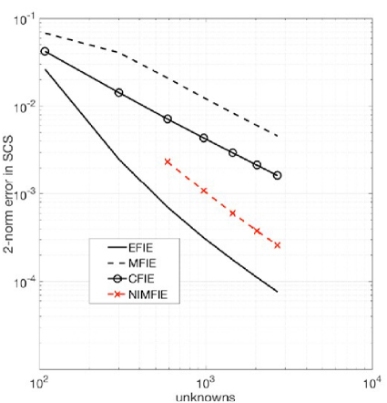
Figure 2: Error in the SCS for a sphere with ka$\mathrm{=}$2$\pi$.

We next consider several examples whose surfaces contain sharp or abrupt bends and tips. Figure 3 shows the magnitude of the surface current density for a perfectly conducting missile target [14] with surface area 25${\lambda }^2$, obtained from the EFIE, MFIE, and NIMFIE equations with a 2592-cell model. The target is illuminated nose-on with a horizontally-polarized incident electric field. This target has two fin-like protrusions containing 90-degree bends. For this example, the NIMFIE result exhibits qualitative agreement with the EFIE result, while the MFIE current shows minor differences.

Table 1: 2-norm errors in the results for the missile

	J Error	E-residual	SCS Error
MFIE	17%	27%	3.3%
CFIE	18	19	2.5
NIMFIE	17	22	2.0
EFIE	19	17	0.15

Several measures of the error are reported in Table 1, including the error in the currents obtained by a comparison with a higher order solution of the EFIE, the tangential electric-field residual error [15], and the SCS error compared to a higher order EFIE reference result. The current density error is computed using:

$$J_{err}=\frac{\sqrt{\frac{1}{A_{total}}{\sum }_{n=1}^{N_{cells}}{\left|{\overline{J}}_{n,ref}-{\overline{J}}_{n,RWG}\right|}^2{A}_n}}{2\left|H_{\max }^{inc}\right|},$$

(10)

where A${}_n$ is the area of cell n. These results suggest that all four approaches produce somewhat similar accuracy in the current density, with a 2-norm error around 20%, and that the NIMFIE is slightly better than the MFIE in SCS accuracy.

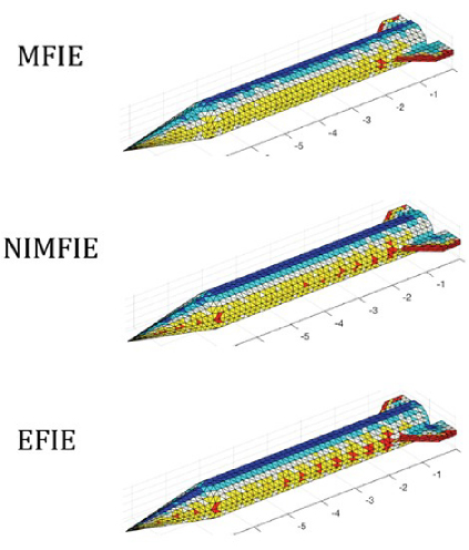
Figure 3: Current density magnitude on a perfectly conducting missile target. Red denotes the largest magnitudes, followed by yellow, white, light blue, and dark blue, on a non-logarithmic scale. The target is illuminated nose-on with a horizontally-polarized incident electric field. The scales are in wavelength.

Figure 4 shows the surface current magnitude on a perfectly conducting cone-sphere with a total length of 5.66$\lambda$, a cone length-to-radius ratio of 4:1, and a total surface area of 25${\lambda }^2$, for a vertically-polarized electric field incident upon the sharp tip end of the target. A 2812-cell model is used. The NIMFIE result exhibits agreement with the EFIE result, while the MFIE result shows some differences. Various error measures are reported in Table 2. The overall errors are smaller for the cone-sphere than the missile, and the SCS error obtained from the NIMFIE results are significantly smaller than those of the MFIE and CFIE.

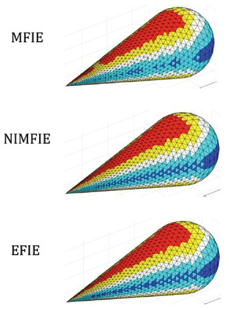
Figure 4: Current density magnitude induced on a perfectly conducting cone-sphere target of surface area 25${\lambda }^2$, by a wave with a vertically polarized electric field incident upon the tip end of the target. Red denotes the largest magnitudes, followed by yellow, white, light blue, and dark blue, on a non-logarithmic scale.

Table 2: 2-norm errors for the cone-sphere target

	J Error	E-residual	SCS Error
MFIE	12%	17%	1.5%
CFIE	12	14	0.80
NIMFIE	11	14	0.24
EFIE	13	13	0.030

Figure 5 shows the magnitude of the surface current on a perfectly conducting “Arrow” target [16] with surface area of 25${\lambda }^2$ and 2002 cells. The bottom of the target is flat, with interior angles of only 36 and 53 degrees around the front and side edges, respectively. The NIMFIE and EFIE results exhibit reasonable visual agreement, while the MFIE result shows differences. Table 3 reports various 2-norm errors. For this target, the NIMFIE SCS error is smaller than that of the MFIE or CFIE, and almost as low as the EFIE SCS error.

Table 3: 2-norm errors for the Arrow target

	J Error	E-residual	SCS Error
MFIE	21%	36%	4.1%
CFIE	19	20	2.1
NIMFIE	17	25	0.78
EFIE	19	21	0.67

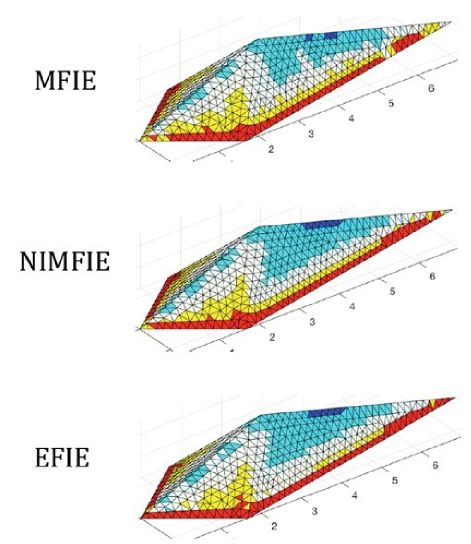
Figure 5: Current density magnitude induced on a perfectly conducting “Arrow” target [16] with surface area of 25${\lambda }^2$. The target is illuminated nose-on with a horizontally-polarized incident electric field. The scales are in wavelength. Red denotes the largest magnitudes, followed by yellow, white, light blue, and dark blue, on a non-logarithmic scale.

Table 4: 2-norm errors for the 2700-cell cube target

	J Error	E-residual	SCS Error
MFIE	42%	83%	8.4%
CFIE	9	9	0.19
NIMFIE	9	11	0.19
EFIE	15	8	0.039

Table 5: Ratio of MFIE SCS error to other equation’s SCS error

Target	Area (${\lambda }^{\mathrm{2}}$)	Density (Cells/${\lambda }^{\mathrm{2}}$)	CFIE	NIMFIE	EFIE
sphere	12.6	108	2.8	16	55
cube #1	15.015	180	44	44	212
almond #1, H-pol	21.8	118	2.5	2.9	28
cube #2	24	113	7.2	7.9	23
missile	25	104	1.3	1.7	22
4:1 cone-sphere	25	112	1.9	6.3	52
Arrow, H-pol	25	80	1.9	5.3	6.2
Arrow, V-pol	25	80	1.5	3.3	5.4
almond #2, V-pol	44.5	104	1.1	9.8	21

Figure 6 shows the magnitude of the current density on a cube target with cube edge length 1.58$\lambda$. This target happens to be internally resonant for the MFIE, and the MFIE result is clearly incorrect. The NIMFIE result for the current magnitude obtained with a 2700-cell model exhibits reasonable agreement with a CFIE result obtained with a 4800-cell model. Table 4 shows several measures of the 2-norm error, obtained from 2700-cell models for the four approaches. For this example, the “resonant-free” NIMFIE and CFIE produce similar error levels in both current and SCS.

Table 5 summarizes the results of the preceding examples and several others in a different manner, by reporting the ratio of the MFIE SCS 2-norm errors to those of the other formulations. The additional targets include a second cube illuminated face-on, the Arrow illuminated by a vertically-polarized incident electric field, and two almond targets illuminated by waves incident on their blunt ends. These results show the disparity between the EFIE and MFIE SCS accuracy in practice. They also suggest that the NIMFIE formulation consistently outperforms the MFIE for SCS error, and almost always produces more accurate SCS results than the CFIE.

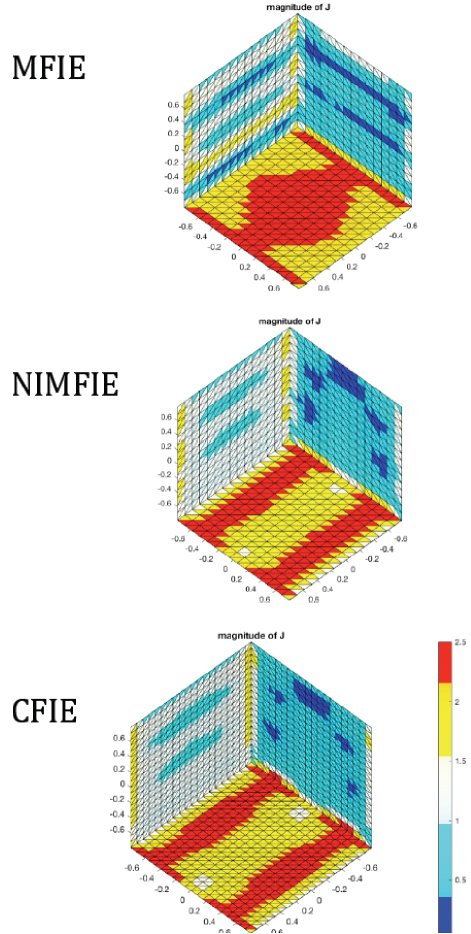
Figure 6: Current density magnitude induced on a perfectly conducting cube target by a wave normally incident on one of the faces. The MFIE and NIMFIE results are obtained with 2700-cell models, while the CFIE result is obtained using a model with 4800 cells. The color scale is non-logarithmic and is a fraction of twice the incident magnetic field.

Table 6 shows the matrix condition numbers reported by the matrix solver for the various approaches and the preceding examples. The CFIE has the lowest (best) condition numbers, while the NIMFIE condition numbers are the same order as those of the EFIE. The data reflect the fact that the “cube #1” target is internally resonant for the MFIE (and apparently close to an internal resonance for the EFIE) and also suggests that there are irregularities associated with the model used for the cone-sphere, probably near the tip.

Table 6: Condition numbers for the cases in Table 5

Target	MFIE	CFIE	NIMFIE	EFIE
sphere	57	21	235	125
cube #1	1918	26	473	9293
almond #1	276	23	469	417
cube #2	91	26	463	143
missile	971	106	1509	1650
cone-sphere	7880	817	13320	12749
Arrow	592	54	2240	1905
almond #2	550	37	846	2170

IV. CONCLUSION

The NIMFIE approach has been implemented with flat-patch models and RWG basis functions, and results for a variety of targets with bends in their surfaces were compared to the traditional MFIE and the CFIE. For these targets, the NIMFIE SCS accuracy is consistently better than that produced by the MFIE and is usually better than the accuracy of the CFIE. These results support the hypothesis that the traditional MFIE discretization, using the “strong” MFIE operator, is more sensitive to surface discontinuities than the “weak” NIMFIE approach. As implemented here, the NIMFIE is free from internal resonances, and it appears to offer advantages over the traditional MFIE formulation.

REFERENCES

[1] S. M. Rao, D. R. Wilton, and A. W. Glisson, “Electromagnetic scattering by surfaces of arbitrary shape,” IEEE Trans. Antennas Propagat., vol. AP-30, no. 3, pp. 409-418, May 1982.

[2] A. E. Ofluoglu, T. Ciftci, and O. Ergul, “Magnetic field integral equation,” IEEE Antennas and Propagation Magazine, vol. 57, no. 4, pp. 134-142, 2015.

[3] A. F. Peterson, “The interior resonance problem associated with surface integral equations of electromagnetics: Numerical consequences and a survey of remedies,” Electromagnetics, vol. 10, no. 3, pp. 293-312, 1990.

[4] A. F. Peterson and M. M. Bibby, An Introduction to the Locally-corrected Nyström Method. San Raphael: Morgan and Claypool Synthesis Lectures, 2010.

[5] O. Ergul and L. Gurel, “Improving the accuracy of the magnetic field integral equation with linear-linear basis functions,” Radio Science, vol. 41, no. 4, RS4004, 2006.

[6] A. F. Peterson, “Observed baseline convergence rates and superconvergence in the scattering cross section obtained from numerical solutions of the MFIE,” IEEE Trans. Antennas Propagat., vol. 56, no. 11, pp. 3510-3515, Nov. 2008.

[7] M. M. Bibby and A. F. Peterson, “Elimination of the derivatives from the conventional MFIE operator,” in Proceedings of the 22${}^{n\mathit{}d}$ Annual Review of Progress in Applied Computational Electromagnetics, Miami, FL, pp. 359-364, Mar. 2006.

[8] M. M. Bibby, C. M. Coldwell, and A. F. Peterson, “Normally-integrated magnetic field integral equations for electromagnetic scattering,” IEEE Trans. Antennas Propagat., vol. 55, no. 9, pp. 2530-2536, 2007.

[9] M. M. Bibby, C. M. Coldwell, and A. F. Peterson, “A high order numerical investigation of electromagnetic scattering from a torus and a circular loop,” IEEE Trans. Antennas Propagat., vol. 61, no. 7, pp. 3656-3661, 2013.

[10] A. F. Peterson and M. M. Bibby, “Performance of the normally-integrated magnetic field integral equation for flat faceted surfaces,” in International Conference on Electromagnetics in Advanced Applications (ICEAA 23), Venice, Italy, Oct.2023.

[11] A. F. Peterson and M. M. Bibby, “Superior far field accuracy of the normally-integrated MFIE compared to the conventional MFIE for flat-faceted targets,” in International Applied Computational Electromagnetics Society (ACES) Symposium, Orlando, FL, May 2024.

[12] M. B. Woodworth and A. D. Yaghjian, “Multiwavelength three-dimensional scattering with dual-surface integral equations,” J. Opt. Soc. Am. A., vol. 11, no. 4, pp. 1399-1413, Apr. 1994.

[13] A. F. Peterson, D. R. Wilton, and R. E. Jorgenson, “Variational nature of Galerkin and non-Galerkin moment method solutions,” IEEE Trans. Antennas Propagat., vol. 44, no. 4, pp. 500-503, Apr. 1996.

[14] S. K. Kim and A. F. Peterson, “Adaptive h-refinement for the RWG based EFIE,” IEEE J. Multiscale and Multiphysics Comp. Tech., vol. 3, pp. 58-65, June 2018.

[15] A. F. Peterson, “Integral equation residuals for error estimation and internal resonance detection,” IEEE Trans. Antennas Propagat., vol. 71, no. 12, pp. 9326-9333, Dec. 2023.

[16] M. E. Kowalski, B. Singh, L. C. Kempel, K. D. Trott, and J.-M. Jin, “Application of the integral equation-asymptotic phase (IE-AP) method to three-dimensional scattering,” J. Electromagnetic Waves Appl., vol. 15, pp. 885-900, July 2001.

BIOGRAPHIES

Andrew F. Peterson received the B.S., M.S., and Ph.D. degrees in Electrical Engineering from the University of Illinois, Urbana-Champaign, USA. Since 1989, he has been a member of the faculty of the School of Electrical and Computer Engineering at the Georgia Institute of Technology, where he is a full Professor. Within ACES, he has served at various times as a member of the Board of Directors, the Finance Committee Chair, the Publications Committee Chair, and the President. He was elevated to ACES Fellow in 2008.

Malcolm M. Bibby received the B.Eng. and Ph.D. degrees in Electrical Engineering from the University of Liverpool, UK, in 1962 and 1965, respectively, and an MBA from the University of Chicago, USA. He is currently an Adjunct Professor in ECE at Georgia Tech. He has been interested in the numerical aspects of antenna design and electromagnetics for more than 40 years.

ACES JOURNAL, Vol. 40, No. 4, 302–308
doi: 10.13052/2024.ACES.J.400403
© 2025 River Publishers