Compressing Electromagnetic Field by Rational Interpolation of the Spherical Wave Expansion Coefficients

Haobo Yuan${}^{\mathbf{\text{1}}}$, Pu Yang${}^{\mathbf{\text{1}}}$, Nannan Wang${}^{\mathbf{\text{1}}}$, Yi Ren${}^{\mathbf{\text{1}}}$, and Shasha Li${}^{\mathbf{\text{2}}}$

¹School of Electronic Engineering
Xidian University, Xi’an, Shaanxi, China
useryuanhaobo@163.com, 3024396382@qq.com, wnannan2001@163.com, yren@xidian.edu.cn

²Beijing Institute of Space Long March Vehicle
Beijing, China
heiyu-kuaidou@hotmail.com

Submitted On: August 4, 2024; Accepted On: April 10, 2025

ABSTRACT

It is of great significance to obtain the electromagnetic field radiated by an antenna or scattered by an object over a frequency band. But this data often occupies so large a memory that cannot be applied readily. This paper proposes to compress the field based on the spherical harmonic transformation (SHT) and rational interpolation. First, the tangential electric field over a sphere surrounding the antenna is obtained by simulation or measurement. Then, this field is converted into the spherical harmonic coefficients, which are sparse discrete spectra. Finally, these coefficients are interpolated over the whole frequency band with only a few sampling points. Numerical examples show that the proposed algorithm can compress the data of the near field of a rectangular waveguide antenna by about 17278 times, and those of the far field scattered from an UAV by about 103 times.

Index Terms: Antenna, data compression, rational interpolation, spherical harmonic transform.

I. INTRODUCTION

The data of the electromagnetic field radiated by an antenna or scattered from an object is widely applied in many engineering scenarios, such as radar imaging, antenna measurement and base station deployment. As shown in Fig. 1, the field often varies rapidly as frequency and scanning angle changes. Therefore, one needs to sample quite densely in both frequency and angle to accurately represent the field. Many compression techniques have been developed to reduce this large amount of data.

The method introduced by Burnside et al. is based on radar imaging technology [1-3]. It extracted the scattering centers according to the radar images. The scattering field from an individual scattering center can be expressed as a complex exponential function of frequency and angle. As a result, the radar cross section (RCS) is compressed drastically. There are some additional methods based on the theory of scattering centers, such as the matrix pencil method [4] and the CLEAN algorithm [5, 6].

Regarding the data of the electromagnetic field as a matrix, one can make use of the well-established image compression algorithms. These algorithms often exploit the low-rank property of a particular matrix. In order to compress the near field data, Wu et al. proposed the CUR decomposition [7] and Zhao et al. proposed the skeletonization-scheme [8]. Guo et al. applied the butterfly scheme [9] to compress the system matrix generated by the combined-field integral equation. The most widespread ones are the threshold discrete Fourier transform (TDFT) method [10, 11] and the truncated singular value decomposition (SVD) method [12, 13].

Another type of compression method applies compressive sensing (CS) [14–19] to reconstruct the antenna radiation pattern in the antenna measurements. The CS process often uses a transform, such as discrete cosine transform or discrete Fourier transform, that renders the data of the field to be a sparse vector in the transform domain. Minimizing the ${\mathit{l}}_{\mathbf{1}}$-norm of this vector will reconstruct the field data with much fewer random measurements. This method sheds some light on the proposed method, which transforms the electromagnetic fields into the spherical harmonic spectra in Fig. 2 by spherical harmonic transformation (SHT). Fortunately, the spherical harmonic spectra are low-pass, discrete and sparse. Furthermore, the $l_{\mathbf{1}}$-norm minimization in CS may be time-consuming if the iterative procedure diverges, whereas SHT is a deterministic algorithm with $O(N^3)$ operations, where $N$ is the truncation order.

Some use SHT to compress the pattern of an antenna. Reference [20] expanded the field by SHT and Slepian decomposition. Reference [21] applied the sparse spherical harmonic expansion with compressed sensing to expand the far field of an antenna. None of them discussed the frequency-sweeping technique, thus the compression ratio for a frequency band will be limited. Reference [22] applied the 2-D scalar SHT and the windowed interpolation for compression. As is discussed in [22], this commonly used rational interpolation method is numerically unstable as the number of sampling points increases. Therefore, the interpolated function may have some spikes in the curve, called “Froissart doublets” [23].

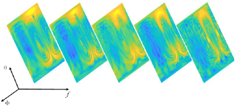
Figure 1: Electric field varies with frequency.

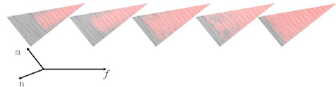
Figure 2: Spherical harmonic spectra vary with frequency.

Since the data of the field is also a function of frequency, we need to implement frequency sweeping efficiently. Reference [24] considered the field radiated by an antenna at a specific angle as a function of frequency, which is expanded by the Chebyshev polynomials. Actually, most of the physical quantities in an electronic system are not polynomials, but rational polynomials. Therefore, this paper applies the rational interpolation based on the Loewner matrix as the frequency sweeping tool.

In summary, the proposed method combines two techniques to compress the data of field in Fig. 1. On the one hand, the field at a specific frequency is converted into spherical harmonic spectra in Fig. 2. On the other hand, the spherical harmonic spectra over a frequency band are approximated by the rational interpolation, which requires the spectra at only a few sampling frequencies.

This paper is organized as follows. Section II introduces the theory of SHT and rational interpolation, and gives the flowchart of the proposed algorithm. Section III validates the proposed algorithm with two numerical examples. Finally, conclusions are drawn in section IV.

II. FORMULATION OF THE ALGORITHM

A. Spherical harmonic transform

Spherical harmonic transform is a well-established algorithm in near-field antenna measurement. The time-harmonic electromagnetic field in a source free space generated by the antenna can be expanded by the spherical harmonics as in [25]:

	$\mathit{E}$	$=-{\displaystyle \sum _{n=1}^N}{\displaystyle \sum _{m=-n}^n}\left(a_{n,m}{\mathit{M}}_{n,m}+b_{n,m}{\mathit{N}}_{n,m}\right),$		(1)
	$\mathit{H}$	$={\displaystyle \frac{-1}{120\pi }}{\displaystyle \sum _{n=1}^N}{\displaystyle \sum _{m=-n}^n}\left(a_{n,m}{\mathit{N}}_{n,m}+b_{n,m}{\mathit{M}}_{n,m}\right),$		(2)

where $\mathit{N}$ is the truncation order of the spherical harmonics, $a_{n,m}$ and $b_{n,m}$ are the spherical harmonic coefficients and the range of subscripts is $1\le n\le N,-n\le m\le n$. The vector spherical harmonics in the spherical coordinate system are:

$${\mathit{M}}_{n,m}=C_{n,m}\cdot \left[\begin{array}{c}\hfill \frac{jm}{\sin \theta }{Z}_n\left(kr\right)P_n^{\left|m\right|}\left(\cos \theta \right)\widehat{\theta }\hfill \\ \hfill -Z_n\left(kr\right)\frac{d}{d\theta }{P}_n^{\left|m\right|}\left(\cos \theta \right)\widehat{\phi }\hfill \end{array}\right]\cdot e^{jm\phi },$$

(3)

$${\mathit{N}}_{n,m}=C_{n,m}\cdot \left\{\begin{array}{c}\hfill \frac{Z_n\left(kr\right)}{kr}n\left(n+1\right)P_n^{\left|m\right|}\left(\cos \theta \right)\widehat{r}\hfill \\ \hfill +W_n\left(kr\right)\left[\begin{array}{c}\hfill \frac{d}{d\theta }{P}_n^{\left|m\right|}\left(\cos \theta \right)\widehat{\theta }\hfill \\ \hfill +\frac{jm}{\sin \theta }{P}_n^{\left|m\right|}\left(\cos \theta \right)\widehat{\phi }\hfill \end{array}\right]\hfill \end{array}\right\}\cdot e^{jm\phi },$$

(4)

where $\mathit{\theta }$ and $\mathit{\phi }$ are the elevation angle and the azimuth angle respectively, $\mathit{n}$ is the degree, m is the order, ${\mathit{P}}_{\mathit{n}}^{\left|\mathit{m}\right|}\left(\mathbf{cos}\mathit{\theta }\right)$ is the associated Legendre function, ${\mathit{Z}}_{\mathit{n}}\mathbf{(}\mathit{k}\mathit{r}\mathbf{)}$ is the spherical Bessel function, k is the wave number of free space, ${\mathit{C}}_{\mathit{n},\mathit{m}}\mathbf{=}{\mathbf{(}\mathbf{-}\mathbf{1}\mathbf{)}}^{\mathit{m}}\sqrt{\frac{\left(\mathbf{2}\mathit{n}\mathbf{+}\mathbf{1}\right)\mathbf{(}\mathit{n}\mathbf{-}\left|\mathit{m}\right|\mathbf{)}\mathbf{!}}{\mathbf{4}\mathit{\pi }\mathit{n}\left(\mathit{n}\mathbf{+}\mathbf{1}\right)\left(\mathit{n}\mathbf{+}\left|\mathit{m}\right|\right)\mathbf{!}}}\mathbf{,}{\mathit{W}}_{\mathit{n}}\left(\mathit{k}\mathit{r}\right)\mathbf{=}\frac{\mathbf{1}}{\mathit{k}\mathit{r}}\frac{\mathit{d}}{\mathit{d}\mathit{r}}\left[\mathit{r}{\mathit{Z}}_{\mathit{n}}\left(\mathit{k}\mathit{r}\right)\right]$.

In the spherical near-field antenna measurement, we acquire the tangential near electric field on a sphere surrounding the antenna by a mechanical scanning procedure:

$$E^{\tan }=E_{\theta }\widehat{\theta }+E_{\phi }\widehat{\phi },$$

(5)

where ${\mathit{E}}_{\mathit{\theta }}$ and ${\mathit{E}}_{\mathit{\phi }}$ are the components of ${\mathit{E}}^{\mathbf{tan}}$ in the $\mathit{\theta }$ and $\mathit{\phi }$ direction. The unknown spherical harmonic coefficients can be evaluated by the following integrals:

$$a_{n,m}=-\frac{C_{n,m}}{Z_n\left(k{r}_0\right)}\left\{\begin{array}{c}\hfill {\int }_0^{\pi }\left[{\int }_0^{2\pi }{E}_{\theta }(r_{0,}\theta ,\phi )e^{-jm\phi }\mathit{d}\phi \right]\hfill \\ \hfill \cdot jm{P}_n^{\left|m\right|}\left(\cos \theta \right)d\theta \hfill \\ \hfill +{\int }_0^{\pi }\left[{\int }_0^{2\pi }{E}_{\phi }(r_{0,}\theta ,\phi )e^{-jm\phi }\mathit{d}\phi \right]\hfill \\ \hfill \cdot \frac{d}{d\theta }\left[P_n^{\left|m\right|}\left(cos\theta \right)\right]\sin \theta d\theta \hfill \end{array}\right\}.$$

(6)

$$b_{n,m}=-\frac{C_{n,m}}{W_n\left(k{r}_0\right)}\left\{\begin{array}{c}\hfill {\int }_0^{\pi }\left[{\int }_0^{2\pi }{E}_{\theta }(r_{0,}\theta ,\phi )e^{-jm\phi }\mathit{d}\phi \right]\hfill \\ \hfill \cdot \frac{d}{d\theta }\left[P_n^{\left|m\right|}\left(\cos \theta \right)\right]\sin \theta d\theta \hfill \\ \hfill +{\int }_0^{\pi }\left[{\int }_0^{2\pi }{E}_{\phi }(r_{0,}\theta ,\phi )e^{-jm\phi }\mathit{d}\phi \right]\hfill \\ \hfill \cdot jm{P}_n^{\left|m\right|}\left(\cos \theta \right)d\theta \hfill \end{array}\right\}.$$

(7)

The above double integral consists of an inner integral and an outer integral. The inner integral is just a Fourier integral respect to , which can be evaluated efficiently by the Fast Fourier Transform (FFT). The outer integral is usually calculated by a Gaussian Quadrature. Given the near fields of the antenna, acquiring the spherical harmonic coefficients by (6) and (7) is referred to as the forward SHT. Given the spherical harmonic coefficients of the antenna, evaluating the near fields by (1) is called the inverse SHT. Owing to the FFT, both forward SHT and inverse SHT have the computational complexity of $O(N^3)$, which can be reduced to $O(N^2\log N)$by a novel fast SHT [26].

The expansion coefficients $a_{n,m}$ and $b_{n,m}$ are also termed the spherical harmonic spectra of the electromagnetic field. These are low-pass and discrete spectra which can be stored easily. Because $1\le n\le N,-n\le m\le n$, the number of coefficients $a_{n,m}$ is $N\times (N+2)$, and it also applies for $b_{n,m}$. According to [26], we often take $N=kd+10$, where $d$ is the size of the antenna; the memory requirement for this spectrum is trivial.

Furthermore, among all the $2N\times (N+2)$ coefficients, only a small portion are relatively large quantities, whereas the rest are so small they can be neglected. Therefore, if we only store the non-zero coefficients, then the memory requirement could be reduced significantly. The sparsity pattern of these coefficients is shown in Figs. 12 and 13.

Obviously, (6) and (7) are applied to represent the near field at a single frequency. Often we need the field over a wide frequency band, which will be addressed by a frequency sweeping algorithm called rational interpolation based on Loewner matrix [27, 28].

B. Rational interpolation respect to frequency

Consider only one of the coefficients $a_{n,m}$ and $b_{n,m}$. This coefficient is denoted by $x\left(s\right)$, where $s$ represents the frequency. Suppose $2p-1$ sampling data have been obtained by the forward SHT for the near field of an antenna:

$$x\left(s_i\right)=x_i,i=1,2,3,\mathrm{\cdots },2p-1,$$

(8)

where $s_1<s_2<\mathrm{\cdots }<s_{2p-1}$ are the sampling frequenci-es. We partition these data into two groups:

	$x\left({\lambda }_i\right)$	$=w_i,i=1,2,3,\mathrm{\cdots },p,$		(9)
	$x\left({\mu }_j\right)$	$=v_j,j=1,2,3,\mathrm{\cdots },p-1.$		(10)

With (9), $x\left(s\right)$ can be expressed by the following rational approximation in barycentric form:

Subsequently, we have:

$$\sum _{i=1}^p\frac{v_j-w_i}{{\mu }_j-{\lambda }_i}{\alpha }_i=0,$$

(13)

which is written in compact matrix form as:

$$\left[\begin{array}{ccc}\hfill \frac{v_1-w_1}{{\mu }_1-{\lambda }_1}\hfill & \hfill \mathrm{\cdots }\hfill & \hfill \frac{v_1-w_p}{{\mu }_1-{\lambda }_p}\hfill \\ \hfill \mathrm{⋮}\hfill & \hfill \frac{v_j-w_i}{{\mu }_j-{\lambda }_i}\hfill & \hfill \mathrm{⋮}\hfill \\ \hfill \frac{v_{p-1}-w_1}{{\mu }_{p-1}-{\lambda }_1}\hfill & \hfill \mathrm{\cdots }\hfill & \hfill \frac{v_{p-1}-w_p}{{\mu }_{p-1}-{\lambda }_p}\hfill \end{array}\right]\left[\begin{array}{c}\hfill {\alpha }_1\hfill \\ \hfill \mathrm{⋮}\hfill \\ \hfill {\alpha }_p\hfill \end{array}\right]=0.$$

(14)

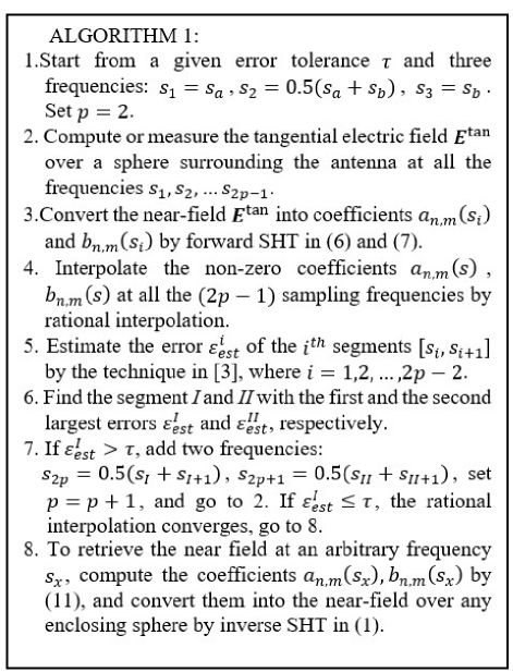
Figure 3: Flowchart of the compression algorithm.

The system matrix on the left side of (14) is the so-called Loewner matrix based on the adopted partition of the samples, and the unknown coefficients ${\alpha }_i$can be readily evaluated by the SVD of the Loewner matrix. Then, the rational polynomial (11) goes through all the $2p-1$ points, and can be viewed as an approximation of the unknown function $x\left(s\right)$.

C. Compressing the field of an antenna or scatterer

The above rational interpolation is suitable for the scalar function, and can be generalized to interpolate a vector function, such as the vector containing all the coefficients $a_{n,m}$ and $b_{n,m}$, for a frequency band $s\in [s_a,s_b]$. More details are given in [3].

The flowchart Fig. 3 presents the algorithm to compress the field of an antenna. It mainly includes four components. The first one is to obtain the tangential near electric field over a sphere surrounding the antenna by computational electromagnetic algorithms or measurements. The second one is the forward SHT in part A. The third one is the rational interpolation in part B. And the last one is the inverse SHT in part A. All together, we can compress the field into the spherical harmonic coefficients and retrieve the field at any frequency efficiently.

III. NUMERICAL RESULTS

The proposed method is validated with the field radiated by a waveguide antenna and the field scattered from an UAV. As the frequency changes, the field of the former varies slightly, while those of the latter varies rapidly. Therefore, we investigate the former over a wide band and the latter over a narrow band. In order to evaluate the accuracy of the compression methods, we define the relative error as:

$$ϵ=\sqrt{\frac{{\sum }_{j=1}^M{\sum }_{i=1}^N{\left|E_c({\theta }_i,{\phi }_j)-E_r({\theta }_i,{\phi }_j)\right|}^2}{{\sum }_{j=1}^M{\sum }_{i=1}^N{\left|E_r({\theta }_i,{\phi }_j)\right|}^2}},$$

(15)

where ${\theta }_i,{\phi }_j$ are the sampling points along the two angles in the spherical coordinate, $M$ and $N$ are the corresponding number of points, $E_c$ represents the electric field obtained by a compression method, and $E_r$ represents the reference field, which is obtained by MoM directly. Furthermore, the definition of compression ratio (CR) is [28]:

$$CR\mathbf{=}\frac{sizeoftheoriginaldata}{sizeofthecompressiondata}.$$

(16)

A. Rectangular waveguide antenna

Figure 4 shows the structure of a WR187 rectangular waveguide antenna, which has an aperture of 47.55$\times$22.15 mm, and is 180 mm in length. This antenna operates at C-band between 4 GHz and 6 GHz. The proposed algorithm is implemented to compress and restore the near field. It is pointed out that the tangential electric field ${\mathit{E}}^{\tan }$ over the enclosing sphere is obtained by MoM, which is the second step of the algorithm. The radius of the sphere is 150 mm, and the truncation order in SHT is $N=14$.

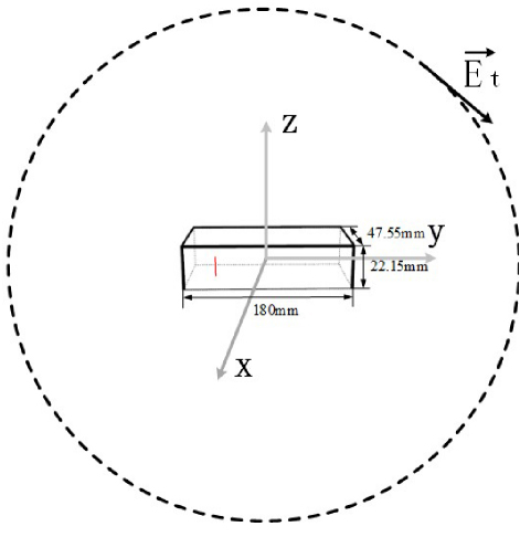
Figure 4: Waveguide antenna and enclosing sphere.

Subsequently, the near field is converted into spherical wave expansion coefficients. Among all the 448 coefficients, there are only 102 non-zero ones, as shown in Figs. 5 and 6. These coefficients are fitted by the rational interpolation with only 11 frequencies and the tolerance in Fig. 3 is $\tau =0.03$. In other words, the MoM simulation is implemented 11 times. Figures 7 and 8 show that the real and imaginary parts of the interpolated $a_{1,1}$ and $b_{14,7}$ are almost identical to the reference. Therefore, the spherical wave expansion coefficients at an arbitrary frequency in the band can be predicted by (10). For example, we compute the coefficients at 5.33 GHz, then restore the near electric field on the enclosing sphere by inverse SHT. Figures 9 and 10 show that the near-field is in good agreement with the reference result.

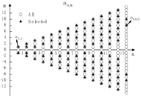
Figure 5: Sparsity of spherical harmonic spectra $a_{n,m}$.

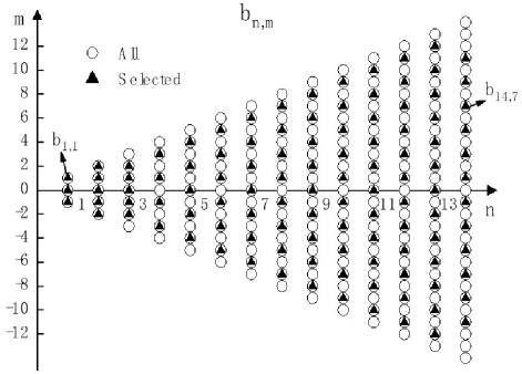
Figure 6: Sparsity of spherical harmonic spectra $b_{n,m}$.

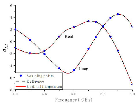
Figure 7: Rational interpolation of the coefficient a${}_{1,1}$.

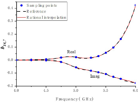
Figure 8: Rational interpolation of the coefficient b${}_{14,7}$.

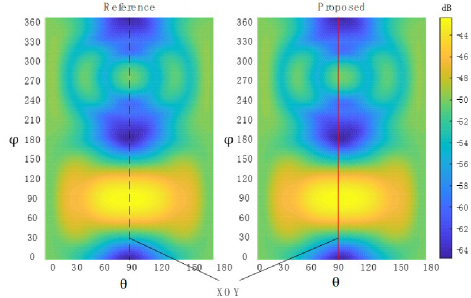
Figure 9: Near-field of waveguide antenna at 5.33 GHz.

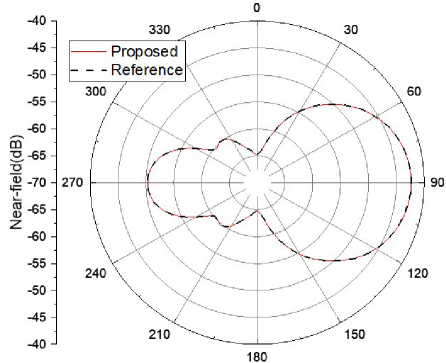
Figure 10: Near-field of waveguide antenna in XOY cut at 5.33 GHz.

Finally, the compression ratio of the near-field is considered. First, we evaluate the memory requirement of the near field without compression. Suppose there are 200 uniformly distributed frequencies from 4 GHz to 6 GHz, and the field at each frequency has 360 azimuthal points and 180 elevational points on the surrounding sphere. Then the memory requirement of the near-field complex vectors is 200$\times$360$\times$180$\times$3$\times$16$\approx$622 MB. Thus, the proposed method needs only 11 frequencies over the whole band, and each frequency has only 102 non-zero spherical wave expansion coefficients. The memory requirement is 11$\times$102$\times$2$\times$16$\approx$0.036 MB, which is negligible. Therefore, the compression ratio is about 17278.

B. UAV RCS

Figure 11 shows the model of a UAV, which is about 5 m in length. The UAV is illuminated by a plane wave ${\mathit{E}}^{\mathrm{inc}}=\widehat{z}{e}^{-jky}$, and the operating frequency band is from 1180 MHz to 1220 MHz. The proposed algorithm will be applied to compress the bistatic RCS of the UAV. Similarly, the second step of the algorithm is computing the tangential near-field ${\mathit{E}}^{\tan }$ of the UAV over the enclosing sphere by MoM. The radius of the sphere is 5 m, and the truncation order in SHT is $N=139$.

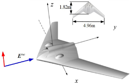
Figure 11: Structure of a UAV.

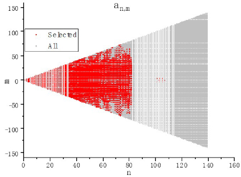
Figure 12: Sparsity of spherical harmonic spectra $a_{n,m}$.

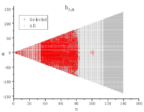
Figure 13: Sparsity of spherical harmonic spectra $b_{n,m}$.

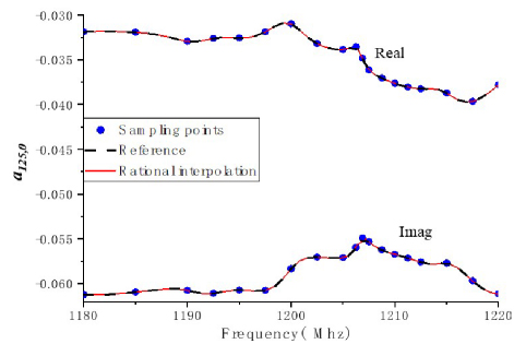
Figure 14: Rational interpolation of coefficient $a_{125,0}$.

Then, the near-field is converted into spherical wave expansion coefficients. There are 15761 non-zero coefficients among all the 39198 coefficients, as shown in Figs. 12 and 13. These non-zero coefficients are interpolated over the frequency band with only 19 frequencies. Figures 14 and 15 show that the real parts and imaginary parts of the interpolated $a_{125,0}$ and $b_{2,-1}$are in good agreement with those of the reference. Also, we compute the coefficients at an arbitrary frequency, say 1216 MHz, by (10), and then restore the far-field or RCS by inverse SHT. Figures 16 and 17 show that the restored far-field is almost the same as the reference result.

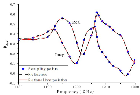
Figure 15: Rational interpolation of coefficient $b_{2,-1}$.

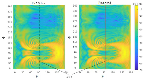
Figure 16: Normalized bi-static RCS of UAV at 1216 MHz.

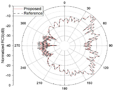
Figure 17: Normalized bi-static RCS of UAV in XOY cut at 1216 MHz.

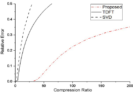
Figure 18: Efficiency of three methods at 1216 MHz.

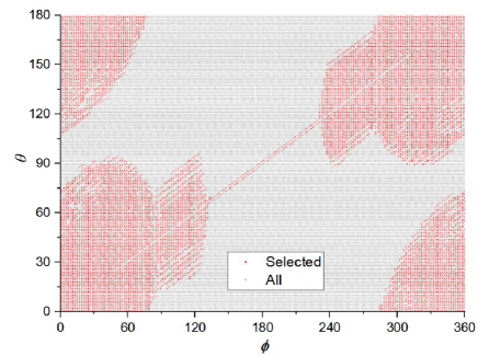
Figure 19: Spectrum of the RCS obtained by TDFT.

Then, the compression ratio is considered. First, we evaluate the memory requirement of the RCS without compression. Suppose there are 40 uniformly distributed frequencies from 1180 MHz to 1220 MHz, and each frequency has 720 azimuthal angles and 360 elevational angles. The memory requirement of the complex vectors will be 40$\times$720$\times$360$\times$3$\times$16$\approx$498 MB. The proposed algorithm needs only 19 frequencies over the whole band, and each frequency has 15761 non-zero spherical wave expansion coefficients. The memory requirement is 19$\times$15761$\times$16$\approx$4.78 MB, and the compression ratio is about 103.

Finally, the efficiency of the proposed algorithm is compared to TDFT [10, 11] and SVD [12, 13] in Fig. 18. Figure 19 shows the spectrum obtained by TDFT, which converts a dense matrix into a sparse one by dropping the small elements in the spectrum matrix. If the relative error is set to be 0.1, the compression ratio of the proposed method is 64.13, while those of TDFT and SVD are 8.71 and 5.21, respectively. Thus, the proposed method is more efficient than the other two methods.

IV. CONCLUSION

This paper gives a novel method to compress the field data of an antenna or a scatterer by SHT and rational interpolation. On the one hand, SHT converts the vectors of near field on a sphere into spherical wave expansion coefficients, which are low-pass sparse discrete spectra. On the other hand, rational interpolation fits these spectra over a frequency band with only a few sampling frequencies. As a result, the data of field are compressed dramatically, and we can readily restore the field data at an arbitrary frequency. This method can efficiently compress both far field and near field.

The proposed method will be improved in the future. First, the spherical wave expansion process will be replaced by FaVeST [24] or the spherical-multipole expansion [29]. Then, the proposed method will be revised to compressing the monostatic RCS, which is more useful in radar imaging and target recognition.

ACKNOWLEDGMENT

This work was supported in part by the Key Research and Development Plan of Shaanxi Province under Grant 2024GX-YBXM-232 and in part by the National Natural Science Foundation of China under Grant U2241203 and 62271365.

REFERENCES

[1] N. Y. Tseng and W. D. Burnside, “A very efficient RCS data compression and reconstruction technique, volume 4,” NASA, Washington, D.C., Tech. Rep. NAS 1.26:191378-Vol-4, Nov. 1992.

[2] L. C. T. Chang, I. J. Gupta, W. D. Burnside, and C. L. T. Chang, “A data compression technique for scattered fields from complex targets,” IEEE Trans. Antennas Propagat., vol. 45, no. 8, pp. 1245-1251, Aug. 1997.

[3] I. J. Gupta and W. D. Burnside, “Electromagnetic scattered field evaluation and data compression using imaging techniques,” NASA, Washington, D.C., Tech. Rep. NAS 1.26:207337, Sep. 1996.

[4] T. K. Sarkar and O. Pereira, “Using the matrix pencil method to estimate the parameters of a sum of complex exponentials,” IEEE Trans. Antennas Propagat., vol. 37, no. 1, pp. 48-55, Feb. 1995.

[5] J. Tsao and B. D. Steinberg, “Reduction of sidelobe and speckle artifacts in microwave imaging: The CLEAN technique,” IEEE Trans. Antennas Propagat., vol. 36, no. 4, pp. 543-556, Apr. 1988.

[6] R. Bhalla and H. Ling, “Three-dimensional scattering center extraction using the shooting and bouncing ray technique,” IEEE Trans. Antennas Propagat., vol. 44, no. 11, pp. 1445-1453, Nov. 1996.

[7] C. Wu, H. Zhao, and J. Hu, “Near field sampling compression based on matrix CUR decomposition,” in APS/URSI, Singapore, pp. 1455-1456, 2021.

[8] H. Zhao, X. Li, Z. Chen, and J. Hu, “Skeletonization-scheme-based adaptive near field sampling for radio frequency source reconstruction,” IEEE Internet Things, vol. 6, no. 6, pp. 10219-10228, Dec. 2019.

[9] H. Guo, Y. Liu, J. Hu, and E. Michielssen, “A butterfly-based direct integral-equation solver using hierarchical LU factorization for analyzing scattering from electrically large conducting objects,” IEEE Trans. Antennas Propagat., vol. 65, no. 9, pp. 4742-4750, Sep. 2017.

[10] G. M. Binge and E. Micheli-Tzanakou, “Fourier compression-reconstruction technique (MRI application),” in Images of the Twenty-First Century. Proceedings of the Annual International Engineering in EMBC, Seattle, WA, pp. 524-525, 1989.

[11] W. X. Sheng, D. G. Fang, J. Zhuang, T. J. Liu, and Z. L. Yang, “Data compression in RCS modeling by using the threshold discrete Fourier transform method,” Chinese Journal of Electronics, vol. 10, no. 4, pp. 557-559, Oct. 2001.

[12] S. J. Li, H. Pang, P. Y. Li, Y. N. Li, and Z. X. Liu, “Image compression based on SVD algorithm,” in CISAI, Kunming, China, pp. 306-309, 2021.

[13] V. Cheepurupalli, S. Tubbs, K. Boykin, and N. Naheed, “Comparison of SVD and FFT in image compression,” in CSCI, Las Vegas, Nevada, pp. 526-530, 2015.

[14] M. L. Don and G. R. Arce, “Antenna radiation pattern compressive sensing,” in MILCOM, Los Angeles, CA, pp. 174-181, 2018.

[15] P. Debroux and B. Verdin, “Compressive sensing reconstruction of wideband antenna radiation characteristics,” Progress In Electromagnetics Research C, vol. 73, pp. 1-8, 2017.

[16] M. Don, “Compressive antenna pattern measurement: A case study in practical compressive sensing,” in 2022 IEEE AUTOTESTCON, National Harbor, MD, pp. 1-9, 2022.

[17] W. Chen, C. Gao, Y. Cui, Y. Q. Jiang, and L. Yang, “A complex RCS calibration data interpolation method based on compressed sensing,” in PIERS - Fall, Xiamen, China, pp. 1295-1299,2019.

[18] H. Zhang, Y. Jiang, and X. Li, “Reconstruction of antenna radiation pattern based on compressed sensing,” Journal of Shanghai Jiaotong Univ. (Sci.), vol. 25, pp. 790-794, July 2020.

[19] A. Massa, P. Rocca, and G. Oliveri, “Compressive sensing in electromagnetics: A review,” IEEE Trans. Antennas Propagat., vol. 57, no. 1, pp. 224-238, Feb. 2015.

[20] W. Dullaert and H. Rogier, “Novel compact model for the radiation pattern of UWB antennas using vector spherical and Slepian decomposition,” IEEE Transactions on Antennas and Propagation, vol. 58, no. 2, pp. 287-299, 2010.

[21] B. Fuchs, L. le Coq, S. Rondineau, and M. D. Migliore, “Fast antenna far-field characterization via sparse spherical harmonic expansion,” IEEE Transactions on Antennas and Propagation, vol. 65, no. 10, pp. 5503-5510, 2017.

[22] R. J. Allard and D. H. Werner, “The model-based parameter estimation of antenna radiation patterns using windowed interpolation and spherical harmonics,” IEEE Transactions on Antennas and Propagation, vol. 51, no. 8, pp. 1891-1906, 2003.

[23] J. Gilewicz and Y. Kryakin, “Froissart doublets in Padé approximation in the case of polynomial noise,” Journal of Computational and Applied Mathematics, vol. 153, no. 1-2, pp. 235-242, 2003.

[24] Z. Du, M. Kwon, D. Choi, and J. Koh, “Radiation pattern reconstruction techniques for antenna,” ICEIC, pp. 143-146, 2008.

[25] J. E. Hansen, Spherical Near-Field Antenna Measurements. London: IET, 1988.

[26] Q. T. le Gia, M. Li, and Y. G. Wang, “Algorithm 1018: FaVeST-fast vector spherical harmonic transforms,” ACM Transactions on Mathematical Software, vol. 47, no. 4, Dec. 2021.

[27] Y. Q. Xiao, S. Grivet-Talocia, P. Manfredi, and R. Khazaka, “A novel framework for parametric loewner matrix interpolation,” IEEE Transactions on Components, Packaging and Manufacturing Technology, vol. 9, no. 12, pp. 2404-2417, Dec. 2019.

[28] Y. Nakatsukasa, O. Sete, and L. N. Trefethen, “The AAA algorithm for rational approximation,” SIAM J. Sci. Comput., vol 40, no. 3, pp. A1494-A1522, 2018.

[29] W. X. Sheng, D. G. Fang, J. Zhuang, T. Liu, and Z. L. Yang, “Comparative study on the data compression in RCS modeling,” in ISAPE, Beijing, China, pp. 573-576, 2000.

[30] G. Giannetti and L. Klinkenbusch, “A numerical alternative for 3D addition theorems based on the bilinear form of the dyadic Green’s function and the equivalence principle,” Advances in Radio Science, vol. 22, pp. 9-15, 2024.

BIOGRAPHIES

Haobo Yuan was born in Tianmen, Hubei, China, in 1980. He received the B.S., M.S., and Ph.D. degrees in electromagnetic fields and microwave technology from Xidian University, Xi’an, China, in 2003, 2006, and 2009, respectively. Since 2006, he has been with the School of Electronic Engineering, Xidian University, where he is an Associate Professor. He was a post-doctoral researcher at the Ohio State University in 2019. His current research interests include computational electromagnetics, antenna measurements, and electromagnetic compatibility.

Pu Yang was born in An’qing, Anhui, China, in 2000. He received the B.S. degree in electronic information engineering from Changchun University of Science and Technology, Changchun, China, in 2018. He is currently pursuing the M.S. degree with Xidian University. His research interests are numerical techniques in computational electromagnetics.

Nannan Wang received the B.S. degree in electronic information engineering from Nanjing University of Information Science and Technology, Nanjing, China, in 2023. She is currently pursuing the M.Eng. degree with Xidian University. Her research interest is antenna measurement techniques.

Yi Ren (Senior Member, IEEE) was born in Anhui, China, in 1982. He received the B.S. degree from Anhui University, Hefei, China, in 2004, and the Ph.D. degree from the University of Electronic Science and Technology of China (UESTC), Chengdu, China, in 2009. In 2009, he joined Chongqing Jinmei Inc., Chongqing, China, as an Electromagnetic Compatibility Engineer. In 2011, he joined the Chongqing University of Posts and Telecommunications (CQUPT), Chongqing, where he was lately promoted as Full Professor. From 2014 to 2015, he was a Post-Doctoral Research Scholar with Duke University, Durham, NC, USA. Since August 2020, he has been a Professor with Xidian University, Xi’an, China. His research interests include computational electromagnetics and electromagnetic compatibility.

Shasha Li received the B.S. degree in electronic engineering from Northwestern Polytechnical University, Xi’an, China, in 2006. She received the Ph.D. degree in signal and information processing from Institute of Acoustics, Chinese Academy of Sciences (IACAS), Beijing, China, in 2012. Currently, she is an Engineer with Beijing Institute of Space Long March Vehicle, Beijing, China. Her current research interests include adaptive signal processing and array signal processing.

ACES JOURNAL, Vol. 40, No. 4, 317–325
doi: 10.13052/2024.ACES.J.400405
© 2025 River Publishers