Magnetic Field Analysis of Trapezoidal Halbach Permanent Magnet Linear Synchronous Motor Based on Improved Equivalent Surface Current Method

Bo Li $^{1}$ , Junan Zhang $^{2}$ , Xiaolong Zhao $^{2}$ , Zhangyi Miao $^{2}$ , Hao Dong $^{2}$ , and Huijie Li $^{1}$

¹School of Mechatronic Engineering
Xi’an Technology and Business College, Xi’an 710200, China
libo_xatu@163.com

²School of Mechatronic Engineering
Xi’an Technological University, Xi’an 710021, China
88579337@qq.com

Submitted On: September 29, 2024; Accepted On: January 29, 2025

ABSTRACT

This paper proposes an improved analytical method to calculate the two-dimensional air gap magnetic field (AGMF) of the permanent magnet array in trapezoidal Halbach permanent magnet linear synchronous motors. The influence of the trapezoidal magnet bottom angle a, equivalent width coefficient a $_{w}$ , height coefficient a $_{h}$ and air gap height coefficient a $_{g}$ on the amplitude and harmonic distortion rate of the air gap central magnetic field is analyzed. Based on the equivalent surface current method (ESCM), an improved equivalent algorithm based on trapezoidal side length is proposed for the trapezoidal Halbach permanent magnet array (THPMA). The equivalent analytical formula of two-dimensional air gap flux density is derived and verified by the finite element method (FEM). Results show that the improved equivalent surface current method (IESCM) is convenient and accurate and is suitable for magnetic field calculation of irregular magnetic poles with arbitrary section shape. Analysis shows that, compared with a rectangular magnet, when the bottom angle a of the magnet is greater than 90 $^{\circ}$ , AGMF can obtain the maximum peak value of magnetic flux density (B $_{peak}$ ) and the minimum total harmonics distortion of magnetic flux density (THD $_{B}$ ).

Index Terms: Air gap magnetic field, harmonic distortion rate, improved equivalent surface current method (IESCM), permanent magnet linear synchronous motor (PMLSM).

I. INTRODUCTION

A permanent magnet linear synchronous motor (PMLSM) as the core of the power system has the advantages of simple structure, large thrust-to-volume ratio, high efficiency, and accurate positioning. It is highly valued by researchers. With the development of high-end manufacturing, in precision and ultra-precision servo drive systems, applications of PMLSM are used to replace the traditional rotary motor-screw to achieve precise motion and positioning [1–3]. The air gap magnetic field distribution of PMLSM plays an important and decisive role in its performance such as back EMF, thrust, and vibration and noise [4–5]. Therefore, how to accurately analyze the air gap magnetic field of the PMLSM is particularly important to study the amplitude of the air gap magnetic field of the PMLSM and reduce the THD $_{B}$ .

The analysis methods of the air gap magnetic field (AGMF) include numerical and analytical methods. Among them, the numerical method represented by the finite element method (FEM) is mainly used to calculate complex boundary, multiple media, and nonlinear problems. However, the pre-processing and calculation process is time-consuming, and it is generally used to verify electromagnetic performance after the determination of various dimensional parameters. Common analytical methods include equivalent magnetization method, equivalent magnetic circuit method, equivalent magnetic network method, conformal mapping method, and equivalent surface current method (ESCM). References [6–8] use the equivalent magnetization method to calculate the no-load AGMF of PMLSM. By optimizing the shape and size of the permanent magnet, sinusoidal distribution of the no-load AGMF of the motor is improved; however, this method is only applicable to the solution of the electromagnetic field of regular magnet shape whose boundary is parallel to the coordinate axis, the medium is required to be uniform, and the constraint condition that the magnetization direction is completely parallel to the direction of the coordinate system must be satisfied. Therefore, the secondary magnetic field of the motor often needs to be simplified by the equivalent magnetization method, which can cause large errors in calculation of AGMF. The equivalent magnetic circuit method has the advantages of intuitive physical concept, simple to use, and fast calculation speed. References [9–10] use the method to divide the magnetic field to be solved into several independent elements, calculate the magnetic conductivity of each element, and then form a magnetic network model through connecting nodes to calculate the magnetic circuit, and compare the calculation results with FEM. However, the method is difficult with small structures; for example, when modeling the motor magnetic field, it is necessary to consider the small changes in the magnetic network structure caused by the changes of the primary and secondary relative positions. The equivalent magnetic network method considers the local saturation effect of magnetic circuit according to the principle of equivalent flux tube. In references [11–12], the motor is divided into several independent unit magnetic fields with uniform medium and regular geometry to calculate equivalent magnetic conductivity. According to the similarity between the magnetic network and the electrical network, the magnetic network is calculated by the node method, and the air gap magnetic density distribution is obtained. However, the method struggles to solve the magnetic conductivity of adjacent nodes, the amount of data calculation before and after the nodes move is large, and the calculation model lacks universality. The conformal mapping method is similar to the numerical method. References [13–15] use this method to calculate the normal and tangential magnetic flux density of the secondary magnetic field. The method is suitable for homogeneous and isotropic fields, but does not consider the saturation effect, so the accuracy of the magnetic field distribution in the solution domain of the permanent magnet is not high.

ESCM is an effective method to calculate the magnetic field of a permanent magnet. The method regards the interior of the permanent magnet as a vacuum, and the magnetic field generated by the permanent magnet is equivalent to the magnetic field generated by its surface current layer. The method does not consider the complex calculation inside the magnet but converts the complex shape magnet to the current layer magnetic field calculation on its corresponding surface, effectively improving calculation accuracy. Reference [16] analyzed and calculated the primary and secondary magnetic fields of PMLSM of a trapezoidal Halbach permanent magnet array (THPMA) and analyzed and optimized the influence of secondary structure parameters on AGMF. In reference [17], the analytical formula of the space magnetic field of a single permanent magnet is derived by using this method. The expression of the secondary magnetic field of the conventional PMLSM is obtained by coordinate transformation and compared with the finite element simulation results. References [18–20] analyze the magnetic field of PMLSM by using this method, establish the magnetic field models generated by armature winding and permanent magnet, respectively, and obtain the air gap flux density of the motor. It can be seen from the above analysis that the accuracy of various AGMF calculation methods is greatly affected by the geometry of the permanent magnet, resulting in low accuracy of the calculation results which cannot reflect the internal characteristics of the real AGMF. Especially when the geometry of the permanent magnet is irregular and the magnetization direction is complex to rotate, calculation difficulty and deviation of AGMF are particularly obvious. In addition, research on the amplitude (B $_{peak}$ ) and THD $_{B}$ of AGMF in PMLSM with rectangular permanent magnet structure is relatively sufficient. Limited by the rectangular permanent magnet structure, research results are limited to the case that the bottom angle is equal to 90 $^{\circ}$ . However, a trapezoidal permanent magnet (TPM) changes the rectangular structure of the traditional rectangular permanent magnet, resulting in the need to consider the influence of the trapezoidal bottom angle in AGMF calculation. Existing research on the influence of permanent magnet structure with bottom angle not equal to 90 $^{\circ}$ on the B $_{peak}$ and THD $_{B}$ in AGMF has not been shown.

In summary, to accurately calculate the AGMF of a trapezoidal Halbach PMLSM and reveal the influence law of the TPM bottom angle on AGMF B $_{peak}$ and THD $_{B}$ , this paper takes the two-dimensional AGMF of the secondary of the U-shaped PMLSM as the research object and, based on the ESCM, an improved equivalent algorithm with the trapezoidal side length as the unit is proposed for the THPMA. The equivalent analytical formula of two-dimensional air gap magnetic density is derived and verified by FEM. At the same time, the influence law of trapezoidal magnet bottom angle, equivalent width coefficient a $_{w}$ , height coefficient $a_{h}$ and air gap height coefficient a $_{g}$ on amplitude change, and THD $_{B}$ of the central magnetic field in the air gap are analyzed.

II. MODEL OF THPMA

The three-dimensional topology of the THPMA studied in this paper is shown in Fig. 1. The secondary is composed of back iron and TPM. Because the bilateral secondary of the motor is ”U” shape and arranged neatly, the magnetization direction of the adjacent permanent magnets is 90 $^{o}$ different. Therefore, we take one of the symmetrical Halbach array periods for research, as shown by the red box in Fig. 1.

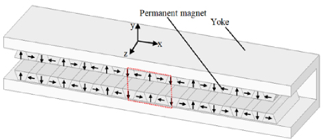
Figure 1: Three-dimensional structure diagram of THPMA.

It can be seen that THPMA is strictly symmetrical along the center of the vertically magnetized permanent magnet in one cycle, so the vertically magnetized permanent magnet is set as the main magnetic pole. AGMF changes as the bottom angle a(0 $\leq$ a $\leq$ $π$ /2, $π$ /2 $\leq$ a $\leq$ $π$ ) of the trapezoidal magnet changes. Generally, the length of the permanent magnet is much larger than the other two directions. Therefore, the three-dimensional model can be equivalent to the two-dimensional model, as shown in Figs. 2 (a) and (b). The center of symmetrical main magnetic pole is the y-axis, the center line of the air gap is the x-axis, magnet height is h, air gap height is g, pole pitch is $τ$ , and waist width of the main magnetic pole is the equivalent width w.

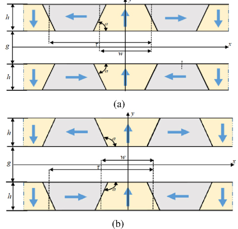
Figure 2: Two-dimensional structure diagram of THPMA: (a) a $<$ 90 $^{\circ}$ and (b) a $>$ 90 $^{\circ}$ .

When solving the AGMF generated by the above secondary array, the following assumptions are made for the magnetic field:

(1) The secondary array of the motor is infinitely long along the x axis.

(2) The magnetic permeability of the secondary yoke of the motor is infinite.

(3) The magnetization of the permanent magnet is uniform, and its relative permeability $μ_{r} =$ 1.

III. IMPROVED EQUIVALENT SURFACE CURRENT METHOD (IESCM) MODELING AND CALCULATION RESULTS

In order to make the research method universal, the model parameters are dimensionless and the characteristic length is $τ$ . The following three dimensionless structure coefficients can be obtained: equivalent width coefficient a $_{w}$ , a $_{w}$ $=$ w/ $τ$ ; height coefficient a $_{h}$ , a $_{h}$ $=$ h/ $τ$ ; air gap height coefficient a $_{g}$ , a $_{g}$ $=$ g/ $τ$ .

A. Model of IESCM

According to ampere molecular circulation hypothesis, the magnetic field at any point in the external space is excited by all the molecular currents neatly arranged in the permanent magnet. Because the permanent magnet is uniformly magnetized, the effect of molecular current in the permanent magnet counteracts each other, so the permanent magnet has only surface current but no body current in the macro view. Based on the above hypothesis, the surface current method is an equivalent method to solve the magnetic field of a permanent magnet by using the solved surface current magnetic field instead of the magnetic field of a permanent magnet. The common equivalent process is to take a single magnet as the basic element, solve the equivalent magnetic field and calculate by superposition. The IESCM proposed in this paper takes any side length of the permanent magnet section as the basic element, calculates the equivalent magnetic field of each side length in the period of magnetic pole array, and then performs the superposition. Because IESCM takes the arbitrary side length of the permanent magnet section as the basic element, it breaks through the calculation constraints of the traditional regular magnet shape and can be used to calculate the irregular magnetic poles with arbitrary section shape in principle. Figure 3 shows the analytical model of trapezoidal Halbach pole structure established by using the IESCM. The two-dimensional absolute rectangular coordinate system xoy is established with the air gap center as the x-axis and the symmetric center of the main magnetic pole as the y-axis.

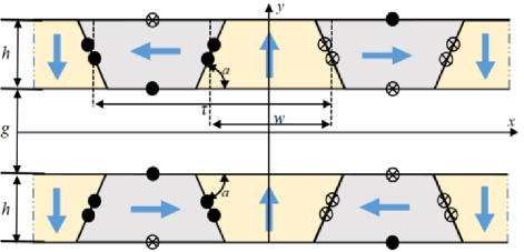
Figure 3: Analytical model of THPMA by IESCM.

The relative coordinate system x $_{t}$ o $_{t}$ y $_{t}$ is established for the side length of each magnetic pole in a cycle. The center of the side length is o $_{t}$ , and the direction of y $_{t}$ forms an acute angle $a_{v}$ with the magnetization direction. Taking the main magnetic pole magnetized vertically upward as an example, the two-dimensional local rectangular coordinate system x $_{t}$ oy $_{t}$ as shown in Fig. 4 is established for the side length I and II of the surface current formed by the two oblique edges of the main magnetic pole, when the bottom angle a of the trapezoidal is 0 $\leq$ a $\leq$ $π$ /2, the right inclined edge of magnetization in $+$ y direction is equivalent to current inflow, and the left inclined edge is equivalent to current outflow.

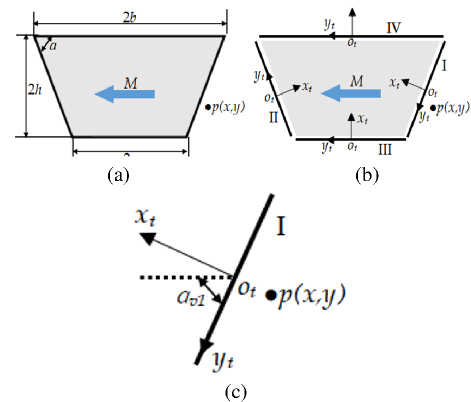
Figure 4: Schematic diagram of -x magnetization coordinate rotation: (a) horizontal left magnetization, (b) relative coordinate system established by side length, and (c) angle $α$ $_{v}$ $_{1}$ between side I and the magnetizing direction.

For any point p(x, y) in AGMF, it can be seen from Fig. 4 that the magnetic field generated by the surface current side I to p(x, y) in AGMF is:

$\begin{matrix} B_{1 x_{t}} (x, y, x_{0 t}, y_{0 t}, α_{v 1}, L_{1}, α_{1}) = \frac{M μ_{0} \cos α_{v 1}}{4 π} ∙ \\ \ln \frac{\begin{matrix} {(- (x - x_{0 t}) \sin α_{1} + (y - y_{0 t}) \cos α_{1} + L_{1} / 2)}^{2} + \\ {((x - x_{0 t}) \cos α_{1} + (y - y_{0 t}) \sin α_{1})}^{2} \end{matrix}}{\begin{matrix} {(- (x - x_{0 t}) \sin α_{1} + (y - y_{0 t}) \cos α_{1} - L_{1} / 2)}^{2} + \\ {((x - x_{0 t}) \cos α_{1} + (y - y_{0 t}) \sin α_{1})}^{2} \end{matrix}} \end{matrix} .$		(1)
$\begin{matrix} B_{1 y_{t}} (x, y, x_{0 t}, y_{0 t}, α_{v 1}, L_{1}, α_{1}) \\ = \frac{M μ_{0} \cos α_{v 1}}{2 π} (\arctan \frac{(y - y_{0 t}) \cos α_{1} - L_{1} - (x - x_{0 t}) \sin α_{1}}{(x - x_{0 t}) \cos α_{1} + (y - y_{0 t}) \sin α_{1}} - \\ \arctan \frac{(y - y_{0 t}) \cos α_{1} + L_{1} - (x - x_{0 t}) \sin α_{1}}{(x - x_{0 t}) \cos α_{1} + (y - y_{0 t}) \sin α_{1}}) \end{matrix} .$		(2)

Similarly, the magnetic field generated by the surface current II is:

(x $_{0 t}$ , y $_{0 t}$ ) is the origin coordinate of the migration coordinate system. L $_{1}$ , L $_{2}$ are side length of the surface current. a $_{1}$ , a $_{2}$ are angles of rotation relative to the coordinate system. a $_{v 1}$ , a $_{v 2}$ are acute angles between the magnetization direction and y $_{t}$ . B $_{1 x t}$ , B $_{1 y t}$ , B $_{2 x t}$ , B $_{2 y t}$ are coordinate directions in the migration coordinate system. The magnetic induction intensity component of the surface current edge of any equivalent current edge I in the principal coordinate system at the p(x, y) is:

${\begin{matrix} B_{i n, x} (x, y, x_{i}, y_{i}, α_{v i}, L_{i}, α_{i}) = \\ B_{1 x_{i}} (x, y, x_{i}, y_{i}, α_{v i}, L_{i}, α_{i}) \cos α_{i} \\ - B_{1 y_{i}} (x, y, x_{i}, y_{i}, α_{v i}, L_{i}, α_{i}) \sin α_{i} \\ B_{i n, y} (x, y, x_{i}, y_{i}, α_{v i}, L_{i}, α_{i}) = \\ B_{1 x_{i}} (x, y, x_{i}, y_{i}, α_{v i}, L_{i}, α_{i}) \sin α_{i} \\ + B_{1 y_{i}} (x, y, x_{i}, y_{i}, α_{v i}, L_{i}, α_{i}) \cos α_{i} \end{matrix} .$		(5)
${\begin{matrix} B_{o u t, x} (x, y, x_{i}, y_{i}, α_{v i}, L_{i}, α_{i}) = \\ B_{2 x_{i}} (x, y, x_{i}, y_{i}, α_{v i}, L_{i}, α_{i}) \cos α_{i} \\ - B_{2 y_{i}} (x, y, x_{0 i}, y_{0 i}, α_{v i}, L_{i}, α_{i}) \sin α_{i} \\ B_{o u t, y} (x, y, x_{i}, y_{i}, α_{v i}, L_{i}, α_{i}) = \\ B_{2 x_{i}} (x, y, x_{i}, y_{i}, α_{v i}, L_{i}, α_{i}) \sin α_{i} \\ + B_{2 y_{i}} (x, y, x_{i}, y_{i}, α_{v i}, L_{i}, α_{i}) \cos α_{i} \end{matrix} .$		(6)

If the direction of the equivalent side current of the magnet is inflow, select equation (5). If the direction of the equivalent side current of the magnet is outflow, select equation (6). Thus, the magnetic induction intensity generated by any surface current edge in the model in Fig. 3 to the point p(x, y) in AGMF is equation (5) or (6).

For fixed point p(x, y) in AGMF, the magnetic induction intensity produced by the permanent magnet pole in one cycle is the superposition of the magnetic induction intensity produced by each surface current edge. It can be seen from the number of surface currents in and out in Fig. 3 that a single bilateral Halbach array has a total of 24 sides, from which the midpoint coordinates p(x, y) and a $_{v i}$ , L $_{i}$ , a $_{i}$ relationship is:

\begin{matrix} B_{x} (x, y) = \sum_{i = 1}^{24} B_{i x} (x, y, x_{i}, y_{i}, α_{v i}, L_{i}, α_{i}) \\ B_{y} (x, y) = \sum_{i = 1}^{24} B_{i y} (x, y, x_{i}, y_{i}, α_{v i}, L_{i}, α_{i}) \end{matrix} .

(7)

Similarly, B $_{i x}$ and B $_{i}$ $_{y}$ can select any one of equation (5) and equation (6) according to inflow or outflow of current. THPMA is arranged along the x axis, and its air gap magnetic density is linearly superimposed. The expression of the air gap magnetic density in the x direction and y direction is:

\begin{matrix} B_{x} (x, y) = \sum_{j = 1}^{\pm \infty} \sum_{i = 1}^{24} B_{i x} (x, y, x_{i} + 2 (j - 1) τ, y_{i}, α_{v i}, L_{i}, α_{i}) \\ B_{y} (x, y) = \sum_{j = 1}^{\pm \infty} \sum_{i = 1}^{24} B_{i y} (x, y, x_{i} + 2 (j - 1) τ, y_{i}, α_{v i}, L_{i}, α_{i}) \end{matrix} .

(8)

According to Figs. 3 and 4 and equation (8), among the 24 calculated side lengths, the five parameters x $_{i}$ , y $_{i}$ , a $_{v}$ $_{i}$ , L $_{i}$ , a $_{i}$ can be expressed using the four basic parameters a, a $_{w}$ , a $_{h}$ $_{,}$ and a $_{g}$ of the trapezoidal Halbach permanent magnet array proposed in the paper, as shown in equation (9). For example, ${$ $\pm$ ( $τ$ -0.5a $_{w}$ ), $\pm$ $τ$ , $\pm$ 0.5a $_{w}$ $}$ is a set of x $_{i}$ , which takes a $_{w}$ as the variable. It can also be seen from equation (9) that the fundamental difference between a magnet with trapezoidal profile and a magnet with rectangular profile is the introduction of trapezoidal bottom angle, which mainly affects a $_{v}$ $_{i}$ , L $_{i}$ , a $_{i}$ :

In summary, the IESCM based on equation (8) first performs equivalent calculation for each TPM in the THPMA and then uses the transformation relationship between local coordinate system and global coordinate system, the super-position principle, to stack the magnetic fields generated by all surface currents and, finally, calculates the complete AGMF distribution. At the same time, according to equation (9), the influence law of the size parameters of THPMA on AGMF is analyzed.

B. Calculation method of THD $_{B}$

According to AGMF distribution obtained from the above solution, under ideal conditions, the air gap flux density waveform is a standard sine wave. However, due to the design of the permanent magnet structure, a large number of nonlinear flux density harmonics are generated in the air gap flux density waveform, which will cause the actual flux density waveform to be distorted, which is usually characterized by THD $_{B}$ . In this paper, THD $_{B}$ of air gap magnetic density is taken as the characteristic expression of sinusoidal air gap magnetic density:

T H D_{B} = \sqrt{\sum_{n = 1}^{\infty} B_{2 n + 1}^{2}} / B_{1}

where B $_{2 n + 1}$ is the amplitude of the odd harmonic air gap magnetic density and B $_{1}$ is the amplitude of the air gap magnetic density fundamental wave. The amplitude of air gap magnetic density in equation (10) can be calculated by the periodic discrete Fourier coefficient.

C. Calculation results and finite element verification

According to the IESCM model established above, we take the ladder type Halbach permanent magnet array model shown in Fig. 3 (a) as example to verify. The permanent magnet adapted the NdFe42, and the calculation parameters are shown in Table 1.

Table 1: Parameter selection of ladder Halbach permanent magnet array

Structural Parameters of Permanent Magnet	Value
Equivalent width of permanent magnet (w)	7.5 mm
Magnet height (h)	9 mm
Pole pitch ( $τ$ )	15 mm
Air gap height (g)	9 mm
Remanence (B $_{r}$ )	1.32 Tesla
Magnetization (M)	1050955 A/m
Permeability ( $μ$ $_{0}$ )	4 $π$ $\times$ 10 $^{7}$ H/m
Bottom angle of trapezoidal (a)	75 $^{\circ}$

The THPMA shown in Fig. 3 is taken as the analysis object, symmetry center is o, and the calculation results of air gap flux density B $_{x}$ $_{y}$ when g $=$ 9 mm are shown in Fig. 5. It can be seen from Fig. 5 that the magnetic field in the air gap is distributed periodically. When the magnetization directions are consistent, the magnetic field strength of the air gap is large, and the area with the largest magnetic field strength is located at the bottom angle of the TPM, with the maximum value of 1.2 T. When the magnetization direction is opposite, the magnetic field intensity in the air gap is the lowest, and the position with the lowest magnetic field intensity is at the bottom angle of the air gap, with a minimum of 0.2 T.

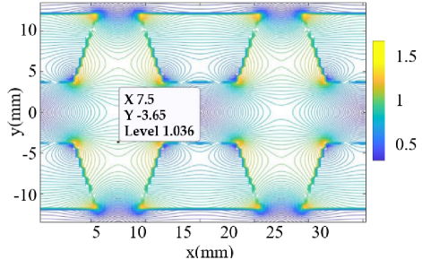
Figure 5: Cloud diagram of AGMF for improved equivalent surface current calculation.

In order to verify the correctness and accuracy of the analytical calculation, FEM is used to simulate the PMLSM secondary model of trapezoidal Halbach magnetization, and the calculation parameters are consistent. The calculation results of IESCM and FEM are shown in Fig. 6.

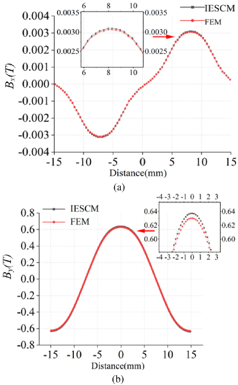
Figure 6: Comparison diagram of single cycle air gap magnetic density FEM and IESCM when g $=$ 9 mm: (a) B $_{x}$ and (b) B $_{y}$ .

It can be seen from Fig. 6 that the analytical method of B $_{x}$ and B $_{y}$ for air gap magnetic density is completely consistent with FEM, but there is error in local size. Based on the simulation results, the maximum relative error is 0.031%. It can be seen from the results that the IESCM proposed in this paper is accurate and effective in calculating the magnetic field of THPMA.

IV. INFLUENCE LAW OF a ON AGMF

The IESCM method is used to calculate AGMF of THPMA, and the correctness of the method is verified by FEM. According to analysis results, a has an important influence on AGMF distribution. This section discusses the influence law of a on B $_{peak}$ and THD $_{B}$ . We reveal the influence law of the coupling effect of a, a $_{w}$ , a $_{h}$ ,and a $_{g}$ , which leads to the maximum value of B $_{peak}$ and the minimum value of THD $_{B}$ . In order to ensure the universality of this research method, take $τ =$ 1, 60 $^{o}$ $\leq$ a $\leq$ 120 $^{o}$ , 0.3 $\leq$ a $_{w}$ $\leq$ 0.7, 0.3 $\leq$ a $_{h}$ $\leq$ 0.7, and 0.3 $\leq$ a $_{g}$ $\leq$ 0.7.

A. Influence law of a, $a_{w}$ , $a_{h}$ , and $a_{g}$ on THD $a_{B}$

Figure 7 (a) shows the three-dimensional topography of THD $_{B}$ with a and a $_{w}$ as variables when a ${}_{h}=$ 0.5 and a ${}_{g}=$ 0.5. It can be seen from Fig. 7 (a), within the parameters of simulation calculation, when a ${}_{h}=$ 0.5 and a ${}_{g}=$ 0.5, the minimum value of THD $_{B}$ is affected by the synergistic effect of a and a $_{w}$ . The isoline of THD $_{B}$ about a and a $_{w}$ shows a V-shaped canyon, the minimum value area is at the bottom of the V-shaped canyon, the minimum value area is located on a straight line composed of a and a $_{w}$ with slope of da/a $_{w}$ , and the maximum value area is at the left and right sides of the V-shaped canyon. The value of THD $_{B}$ on both sides of the canyon presents a symmetrical distribution trend with respect to the V-shaped canyon.

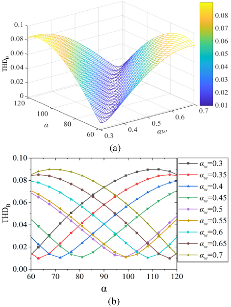
Figure 7: The effect of a and a $_{w}$ on THD $_{B}$ (a $_{h}$ $=$ 0.5, a $_{g}$ $=$ 0.5): (a) three-dimensional topography of THD $_{B}$ with a and a $_{w}$ as variables and (b) analysis of influence law of a and a $_{w}$ on THD $_{B}$ .

Figure 7 (b) shows analysis of the influence law of a and a $_{w}$ on THD $_{B}$ . It can be seen from Fig. 7 (b) that within the parameters of simulation calculation, when a ${}_{w}=$ 0.3, the minimum value of THD $_{B}$ increases with an increase of a. Starting from a ${}_{w}=$ 0.35, with increase of a, the minimum value of THD $_{B}$ first decreases and then increases. When a ${}_{w}=$ 0.7, the minimum value of THD $_{B}$ decreases with the increase of a. The maximum THD $_{B}$ changes with the change of a $_{w}$ . When a $_{w}$ $<$ 0.5, the maximum THD $_{B}$ is located at the side of a $<$ 90 $^{\circ}$ , and when a $_{w}$ $>$ 0.5, its position is exactly the opposite. When a ${}_{w}=$ 0.35 and a $=$ 63.4 $^{\circ}$ , the minimum THD ${}_{B}=$ 0.0098 and the a of maximum THD $_{B}$ is 114 $^{\circ}$ . When a ${}_{w}=$ 0.5 and a $=$ 99 $^{\circ}$ , the minimum THD ${}_{B}=$ 0.0109. The a of maximum THD $_{B}$ is 60 $^{\circ}$ . When a ${}_{w}=$ 0.65 and a $=$ 117 $^{\circ}$ , the minimum THD ${}_{B}=$ 0.0098. The a of maximum THD $_{B}$ is 63.4 $^{\circ}$ .

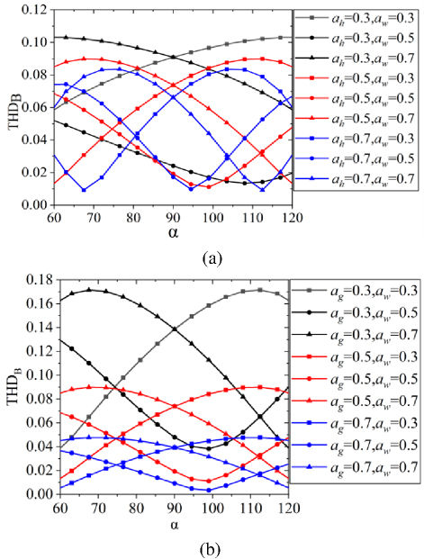
Figure 8: Influence law of a, a $_{h}$ , a $_{g}$ on THD $_{B}$ : (a) change parameters a $_{h}$ (a $_{g}$ $=$ 0.5) and (b) change parameters a $_{g}$ (a $_{h}$ $=$ 0.5).

Figure 8 (a) shows the influence of changing a $_{h}$ on THD $_{B}$ . It can be seen from Fig. 8 (a) that within the parameters of the simulation calculation, the influence of a $_{h}$ on THD $_{B}$ is symmetrically distributed with the change of a, and the amplitude of minimum THD $_{B}$ is not affected by a $_{h}$ but it has an important impact on the amplitude of maximum THD $_{B}$ . The smaller a $_{h}$ , the greater the amplitude of maximum THD $_{B}$ . When a $_{h}$ $=$ 0.3, maximum THD $_{B}$ is 0.103 and minimum THD $_{B}$ is 0.0134. When a $_{h}$ $=$ 0.5, maximum THD $_{B}$ is 0.0899 and minimum THD $_{B}$ is 0.0111. When a $_{h}$ $=$ 0.7, maximum THD $_{B}$ is 0.0835 and minimum THD $_{B}$ is 0.0092. In addition, as a $_{h}$ increases, a will decrease when minimum THD $_{B}$ is obtained. When a $_{h}$ are 0.3, 0.5, and 0.7, respectively, a of minimum THD $_{B}$ are 108 $^{\circ}$ , 99 $^{\circ}$ , and 67.5 $^{\circ}$ , respectively.

Figure 8 (b) shows the influence of changing a $_{g}$ on THD $_{B}$ . It can be seen from Fig. 8 (b) that within the parameters of simulation calculation, the influence of a $_{g}$ on THD $_{B}$ is symmetrically distributed with change of a. The smaller a $_{g}$ , the greater the amplitude of THD $_{B}$ . The change of a $_{g}$ has little effect on a when obtaining the minimum THD $_{B}$ . When a $_{g}$ are 0.3, 0.5, and 0.7, respectively, a of minimum THD $_{B}$ is 98 $^{\circ}$ .

It can be inferred from Figs. 7 and 8 that a has a great influence on THD $_{B}$ amplitude of AGMF, especially when a $\neq$ 90 $^{\circ}$ , a $_{w}$ , a $_{h}$ ,and a $_{g}$ have a common influence on the amplitude of THD $_{B}$ . According to research results, in order to obtain the minimum value of THD $_{B}$ for the traditional rectangular magnet (a $=$ 90 $^{\circ}$ ), a $_{w}$ should be 0.5, which is consistent with the research results in this paper. The change of a changes the intensity of AGMF, which brings distortion to AGMF. Therefore, in magnet design, the influence of the V-shaped canyon composed of a and a $_{w}$ should be considered and appropriate coupling parameters should be selected.

B. Influence law of a, $a_{w}$ , $a_{h}$ , and $a_{g}$ on B $_{peak}$

Figure 9 (a) shows the contour map of B $_{peak}$ impact with a and a $_{w}$ as variables when a $_{h}$ $=$ 0.5 and a $_{g}$ $=$ 0.5. It can be seen from Fig. 9 (a) that within the parameters of simulation calculation, when a $_{h}$ $=$ 0.5 and a $_{g}$ $=$ 0.5, the maximum value of B $_{peak}$ is affected by the synergistic effect of a and a $_{w}$ . The isoline of a and a $_{w}$ on B $_{peak}$ is a hill, and the maximum value area is at the top of the hill, and the value range of a and a $_{w}$ in this area are a $>$ 90 $^{\circ}$ and a $_{w}$ $<$ 0.5.

Figure 9 (b) shows the influence law of a and a $_{w}$ on B $_{peak}$ . It can be seen from Fig. 9 (b) that within the parameters of simulation calculation, when a $_{w}$ $\leq$ 0.5, the maximum value area of B $_{peak}$ increases with the a, and the maximum value area of B $_{peak}$ first increases and then decreases. When 0.3 $<$ a $_{w}$ $<$ 0.45, the maximum value area of B $_{peak}$ gradually increases with the increase of a $_{w}$ , and when 0.45 $<$ a $_{w}$ $<$ 0.5, the maximum value area of B $_{peak}$ gradually decreases with increase of a $_{w}$ . When a $_{w}$ are 0.3, 0.35, 0.4, and 0.5, the corresponding a are 94.5 $^{\circ}$ , 103.5 $^{\circ}$ , 108 $^{\circ}$ , and 117 $^{\circ}$ . Meanwhile, the maximum values of B $_{peak}$ are 0.8797 T, 0.8868 T, 0.8874 T, and 0.8654 T. It should be noted that when a $_{w}$ is equal to 0.4, B $_{peak}$ is at maximum value, and the width of the main magnetic pole is less than 0.5 times pole pitch. Starting from a $_{w}$ $\geq$ 0.5, with increase of a, the maximum value area of B $_{peak}$ gradually increases. With the increase of a $_{w}$ , the maximum value area of B $_{peak}$ gradually decreases. When a $=$ 117 $^{\circ}$ and a $_{w}$ are 0.5, 0.55, 0.6, 0.65, and 0.7, the maximum values of B $_{peak}$ are 0.8684 T, 0.8654 T, 0.8472 T, 0.8242 T, and 0.7972 T.

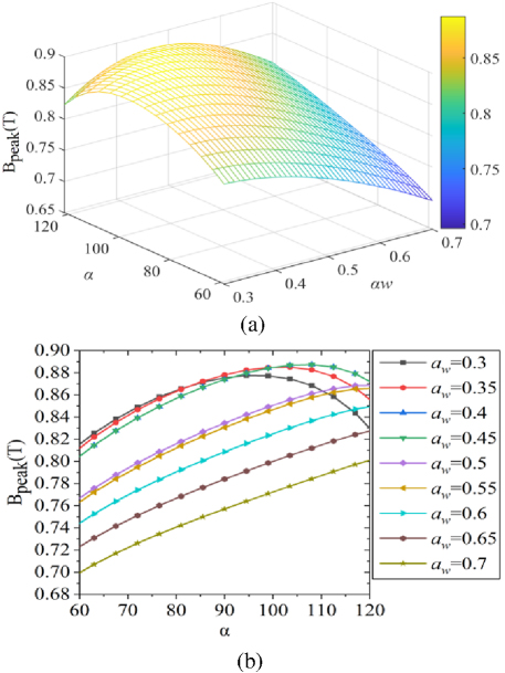
Figure 9: The effect of a and a $_{w}$ on B $_{peak}$ (a $_{h}$ $=$ 0.5, a $_{g}$ $=$ 0.5): (a) three-dimensional topography of B $_{peak}$ with a and a $_{w}$ as variables and (b) analysis of influence law of a and a $_{w}$ on B $_{peak}$ .

Figure 10 (a) shows the effect of changing a $_{h}$ on B $_{peak}$ . It can be seen from Fig. 10 (a) that within the parameters of simulation calculation, a $_{h}$ has an important impact on the influence law of the maximum value of B $_{peak}$ with the change of a. With the increase of a, the greater the a $_{h}$ the greater the maximum value of B $_{peak}$ . When a $_{h}$ are 0.3, 0.5, and 0.7, respectively, the maximum values of B $_{peak}$ are 0.6881 T, 0.8775 T, and 0.9812 T, respectively, and the minimum values of B $_{peak}$ are 0.5574 T, 0.7071 T, and 0.7569 T. In addition, according to Fig. 8 (a), when a $_{h}$ are 0.3, 0.5, and 0.7, respectively, the maximum THD $_{B}$ are 0.103, 0.0899, and 0.0835, and the minimum THD $_{B}$ are 0.0134, 0.0111, and 0.0092. Therefore, on the premise of ensuring the maximum value of B $_{peak}$ and the minimum value of THD $_{B}$ in AGMF, a should be greater than 90 $^{o}$ and a $_{h}$ should be greater than 0.5.

Figure 10 (b) shows the influence of changing a $_{g}$ on B $_{peak}$ . It can be seen from Fig. 10 (b) that within the parameters of simulation calculation, the smaller a $_{g}$ is, the larger B $_{peak}$ is. When a $_{g}$ are 0.3, 0.5, and 0.7, the maximum values of B $_{peak}$ are 1.303 T, 0.8775 T, and 0.6269 T, and the minimum values of B $_{peak}$ are 0.9096 T, 0.7071 T, and 0.5356 T. In addition, according to Fig. 8 (b), when a $_{g}$ are 0.3, 0.5, and 0.7, the minimum THD $_{B}$ is 98 $^{\circ}$ . Therefore, on the premise of ensuring the maximum value of B $_{peak}$ and the minimum value of THD $_{B}$ , a should be greater than 90 $^{\circ}$ and the value range of a $_{g}$ should be 0.3 $<$ a $_{g}$ $<$ 0.5.

It can be further inferred from Figs. 9 and 10 that a has an influence on the amplitude of harmonic distortion rate of AGMF. In order to obtain the maximum value of B $_{peak}$ for traditional rectangular section (a $=$ 90 $^{\circ}$ ), a $_{w}$ should be 0.5 in magnet design. However, when a $\neq$ 90 $^{\circ}$ , in order to ensure the maximum value of B $_{peak}$ and the minimum value of THD $_{B}$ , the values of a, a $_{h}$ , and a $_{g}$ should be a $>$ 90 $^{\circ}$ , a $_{h}$ $>$ 0.5, and 0.3 $<$ a $_{g}$ $<$ 0.5.

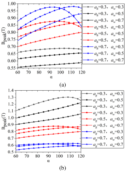
Figure 10: Influence of a, a $_{h}$ , a $_{g}$ on B $_{peak}$ : (a) changing parameters a $_{h}$ (a $_{g}$ $=$ 0.5) and (b) changing parameters a $_{g}$ (a $_{h}$ $=$ 0.5).

V. CONCLUSION

An IESCM for calculating the AGMF of trapezoidal Halbach permanent magnet linear synchronous motor is presented. The calculated results are in good agreement with FEM results, which fully shows the accuracy and practicability of the new analytical method. The method is applicable to the magnetic field analysis of various irregular permanent magnet arrays and has strong reference value for the theoretical analysis of AGMF of other irregular PMLSM.

Taking a, a $_{w}$ , a $_{h}$ , and a $_{g}$ as variables, the minimum value region of THD $_{B}$ is a narrow canyon. Changes of a, a $_{w}$ , and a $_{h}$ significantly affect the trend of the canyon, making the canyon swing and shift, but a $_{h}$ has little effect on the minimum value of THD $_{B}$ . Furthermore, a $_{g}$ mainly affects the steepness of the canyon and the minimum value of THD $_{B}$ . The rectangular magnet of a=90 $^{o}$ is a special case in the change of canyon shape.

B $_{peak}$ of AGMF has a maximum point and a relatively flat maximum neighborhood. Taking the maximum value of B $_{peak}$ of AGMF and the minimum value of THD $_{B}$ of AGMF as optimization objectives, the values of a, a $_{w}$ , a $_{h}$ , and a $_{g}$ are a $>$ 90 $^{\circ}$ , a $_{w}$ $<$ 0.5, a $_{h}$ $>$ 0.5, and 0.3 $<$ a $_{g}$ $<$ 0.5.

ACKNOWLEDGMENT

This work was supported in part by the National Natural Science Foundation of China (51705390); President Fund of Xi’an Technology and Business College (23YZZ08); The 2024 Innovation Training Program for College Students at Xi’an Technology and Business College (202413682001); The Teaching Reform Research Project of Xi’an Technology and Business College in 2024 (24YJZ03).

REFERENCES

[1] W. Xiao-Yuan, H. Xiao-Yu, and G. Peng, “Research on electromagnetic vibration and noise reduction method of V type magnet rotor permanent magnet motor for electric vehicles,” Proceedings of the CSEE, vol. 39, no. 16, pp. 4919-4922, 2019.

[2] C. Liang-Liang, F. Jing-Hong, X. Ru, Z. Chang-Sheng, W. Jia-Ju, and L. Zhi-Nong, “Rotor strength analysis of high-speed surface mounted permanent magnet rotors,” Proceedings of the CSEE, vol. 36, no. 17, pp. 4719-4727, 2016.

[3] D. Jian-Ning, H. Yun-Kai, J. Long, and L. He-Yun, “Review on high speed permanent magnet machines including design and analysis technologies,” Proceedings of the CSEE, vol. 34, no. 27, pp. 4640-4653, 2014.

[4] W. Kai, S. Hai-Yang, Z. Lu-Feng, and L. Chuang, “An overview of rotor pole optimization techniques for permanent magnet synchronous machines,” Proceedings of the CSEE, vol. 37, no. 24, pp. 7304-7317, 2017.

[5] T. Xu, W. Xiu-He, and S. Shu-Min, “Analytical analysis and study of reduction methods of cogging torque in line-start permanent magnet synchronous motors,” Proceedings of the CSEE, vol. 36, no. 5, pp. 1395-1403, 2016.

[6] M. Park, J. Choi, H. Shin, and S. Jang, “Torque analysis and measurements of a permanent magnet type Eddy current brake with a Halbach magnet array based on analytical magnetic field calculations,” Journal of Applied Physics, vol. 115 p. 756, 2014.

[7] J. H. Lee, J. Song, D. Kim, J. Kim, Y. Kim, and S.Y. Jung, “Particle swarm optimization algorithm with intelligent particle number control for optimal design of electric machines,” IEEE Transactions on Industrial Electronics, vol. 99, no. 1-1, 2017.

[8] J. Song, D. Fei, and J. Zhao, “An efficient multi- objective design optimization method for PMSLM based on extreme learning machine,” IEEE Transactions on Industrial Electronics, vol. 66, no. 2, pp. 1001-1011, 2019.

[9] B. Sheikh-Ghalavand, A. Isfahani, and S. Vaez-Zadeh, “An improved magnetic equivalent circuit model for iron-core linear permanent-magnet synchronous motors,” IEEE Transactions on Magnetics, vol. 46, no. 1, pp. 112-120, 2010.

[10] Y. Du, M. Cheng, and K. Chau, “Design and analysis of a new linear primary permanent magnet vernier machine,” Transactions of China Electrotechnical Society, vol. 27, no. 11, pp. 22-30, 2012.

[11] G. Liu, S. Jiang, W. Zhao, and Q. Chen, “Modular reluctance network simulation of a linear permanent-magnet vernier machine using new mesh generation methods,” IEEE Transactions on Industrial Electronics, vol. 64, no. 7, pp. 5323-5332, 2017.

[12] S. Asfirane, S. Hlioui, and Y. Amara, “Global quantities computation using mesh-based generated reluctance networks,” IEEE Transactions on Magnetics, vol. 1, no. 1, pp. 1-4, 2018.

[13] D. Krop, E. Lomonova, and A. Vandenput, “Application of Schwarz-Christoffel mapping to permanent magnet linear motor analysis,” IEEE Transactions on Magnetics, vol. 44, no. 3, pp. 352-359, 2008.

[14] L. Z. Zeng, X. D. Chen, and Q. Xiao, “A thrust force analysis method for permanent magnet linear motor using Schwarz-Christoffel mapping and considering slotting effect, end effect, and magnet shape,” IEEE Transactions on Magnetics, vol. 51, no. 9, pp. 101-108, 2015.

[15] J. Yu, L. Li, and J. Zhang, “Analytical calculation of air-gap relative permeance in slotted permanent magnet synchronous motor,” Transactions of China Electrotechnical Society, vol. 31, no. S1, pp. 45-52, 2016.

[16] M. G. Lee and D. G. Gweon, “Optimal design of a double-sided linear motor with a multisegmented trapezoidal magnet array for a high precision positioning system,” Journal of Magnetism & Magnetic Materials, vol. 281, no. 2-3, pp. 336-346, 2004.

[17] Z. Q. Xue, H. Li, and Z. Yu, “Analytical prediction and optimization of cogging torque in surface mounted permanent magnet machines with modified particle swarm optimization,” IEEE Transactions on Industrial Electronics, vol. 64, no. 12, pp. 9795-9805, 2017.

[18] M. Sun, R. Tong, and X. Han, “Analysis and modeling for open circuit air gap magnetic field prediction in axial flux permanent magnet machines,” Proceedings of the CSEE, vol. 38, no. 5, pp. 1525-1533, 2018.

[19] Z. Guo and R. Shao, “Analytical calculation of magnetic field and cogging torque in surface mounted permanent magnet machines accounting for any eccentric rotor shape,” IEEE Transactions on Industrial Electronics, vol. 62, no. 6, pp. 3438-3447, 2015.

[20] L. Wu, H. Yin, and D. Wang, “A nonlinear subdomain and magnetic circuit hybrid model for open-circuit field prediction in surface mounted PM machines,” IEEE Transactions on Energy Conversion, vol. 34, no. 3, pp. 1485-1495, 2019.

BIOGRAPHIES

Bo Li was born in Shanxi, China. He received the B.S. and M.E. degree in electrical engineering from Xi’an Technological University, China, in 2009 and 2012, respectively. Since 2017, he has been working toward the Ph.D. at the School of Mechatronic Engineering, Xi’an Technological University, Xi’an, China. His current research interests include multi objective design optimization of permanent linear magnet synchronous motors (PMLSM) and fault diagnosis and monitoring in PMLSM.

Junan Zhang was born in Shaanxi, China. He received the B.S. and M.E. degree from Beijing Institute of Technology. In January 1982, he obtained his Ph.D. from Northwestern Polytechnic University in 2006. In 1998, he visited Kyoto technological fiber University in Japan for half a year. Mainly engaged in theoretical research on gas lubrication technology, his current research interests include multi-objective design optimization of permanent magnet synchronous motors (PMSLM), high-performance aerostatic bearings and guide rails.

Xiaolong Zhao was born in Shaanxi, China. He received his Ph.D. degree from Xi’an Technological University. His current research interests include multi-objective design optimization of permanent magnet synchronous motors (PMSLM), and fault diagnosis and monitoring in PMSLM ultra-precision air flotation support technology.

Zhangyi Miao was born in Sanmenxia, Henan, China. Since 2021, he has been studying for a master’s degree in mechanical engineering at Xi’an Technological University. His current research interests include analysis and design of linear motors, design and application of mechanical transmission systems.

Hao Dong was born in Shaanxi, China. He received the B.E. degree in mechanical design, manufacturing and automation from Xi’an Technological University in 2007. He received the M.E. degree in machinery manufacturing and automation from Xi’an Technological University in 2010 and Ph.D. in mechanical design and theory from Northwestern University of Technology in 2013. His current research interests include mechanical transmission system dynamics and mechanical transmission system design and application.

Li Huijie was born in Shaanxi, China. He has been studying for a bachelor’s degree in electrical engineering and Automation at Xi’an Technology and Business College since 2021. His current research interests include power electronics and electrical transmission, mechanical transmission system design and applications.