Circularly Polarized Plane Wave Source Implementation in Time-domain Electromagnetic Simulations
Jake W. Liu
Graduate Institute of Photonics and Optoelectronics
National Taiwan University, Taipei 10617, Taiwan
jwliu@ntu.edu.tw
Submitted On: September 21, 2024; Accepted On: December 18, 2024
ABSTRACT
A unified framework for implementing circularly polarized plane wave sources in time-domain electromagnetic simulations is presented. Unlike traditional approaches that require separate settings for the orthogonal components as different sources, our method integrates circular polarization states represented in frequency domain seamlessly into time-domain simulations. We also studied the effectiveness of the approach when broadband sources are used. This framework is applicable to both finite-difference time-domain (FDTD) and pseudospectral time-domain (PSTD) methods.
Index Terms: Circular polarization, finite-difference time-domain (FDTD), pseudospectral time-domain (PSTD).
I. INTRODUCTION
The FDTD method, a widely used numerical technique for solving Maxwell’s equations in the time-domain, is a powerful tool for simulating complex EM phenomena. However, incorporating circular polarization into these time-domain simulations poses specific challenges. These include accurately representing the phase relationships and amplitude ratios of the orthogonal components of the electric field, ensuring numerical stability, and maintaining computational efficiency. While there is extensive literature on the general application of FDTD, there is a noticeable gap when it comes to practical, detailed guidance on simulating circularly polarized waves.
Modeling circular polarization accurately in EM simulations is crucial for several reasons. Firstly, these polarization states are often used in modern communication systems, where they can enhance signal quality and reduce interference [3]. Secondly, in remote sensing and radar applications, the ability to accurately simulate these polarizations can improve the detection and characterization of various targets and materials [2]. Lastly, in antenna design, understanding the behavior of circularly and elliptically polarized waves can lead to more efficient and effective antenna configurations [4–6].
This paper aims to address the gap in the current literature by providing a comprehensive methodology for implementing circular polarization in time-domain simulations using the collocated Fourier PSTD method, particularly with the introduction of plane wave sources by the total-field scattered-field (TFSF) formulation. The proposed method aims to achieve accuracy within 1% error when comparing the average radius of the electric field intensity to the reference radius. The reason we chose Fourier PSTD over FDTD is in its collocated grid-nature in field calculation, which is much easier for us to verify our results. However, the proposed method is applicable for both FDTD and PSTD simulations. We will explore the theoretical foundations of these polarization states, detail the numerical implementation steps, and validate the approach through various simulations.
II. THEORETICAL BACKGROUND
In this section, we first confine our study to monochromatic EM waves, as circular polarizations are predominantly represented and analyzed in the frequency domain. This focus allows us to leverage the well-established theoretical frameworks and mathematical representations of polarization states for single-frequency waves. A subsequent framework is developed in the next section to seamlessly incorporate the frequency-domain representation into time-domain simulation, and further discussion on expanding the method to broadband sources are also discussed.
Polarization describes the orientation of the electric field vector of an EM wave as it propagates through space. It is a fundamental property that significantly influences the wave’s interaction with materials, reflection and transmission characteristics, and reception by antennas. The three primary types of polarization are linear, circular, and elliptical:
(1) Linear polarization: The electric field vector maintains a constant direction as the wave propagates.
(2) Circular polarization: The electric field vector rotates in a circular motion, making one complete revolution per wavelength. It can be right-hand circularly polarized (RHCP) or left-hand circularly polarized (LHCP), depending on the rotation direction and also the definition. Suppose we have a wave propagating in the z-direction, the phasor representation of a circular polarized electric field at a fix point can be represented by:
(1) where denotes taking the real part of its argument, denotes the amplitude of the electric field, being the angular frequency, and and are orthogonal unit vectors. By further calculations, (1) can be written in a pure time-domain representation as:
(2) Here the same wave function (cosines) is used for both and components. This is better for understanding time-domain implementations, since a single pre-defined waveform can be employed for both orthogonal components of the fields by properly introducing a time delay.
(3) Elliptical polarization: This can be viewed as a generalization of circular polarization where the electric field vector traces an ellipse. It is characterized by the ellipticity (ratio of the minor axis to the major axis) and the orientation angle of the ellipse. The mathematical representation of an elliptically polarized wave is:
(3) Comparing with circular polarizations, two things can be observed from the formulation: (i) the amplitudes can be different in and components and (ii) the phase delays (or advances) do not need to have a difference of .
The polarization state of an EM wave can be represented using Jones vectors or Stokes parameters. For simplicity, we focus on Jones vectors in this paper. A Jones vector is a column vector that represents the amplitude and phase of the orthogonal components of the electric field. For an elliptically polarized wave, the Jones vector is represented by:
| (4) |
In our implementation, by specifying the two orthogonal components of the electric field, representation similar to the Jones vector can be utilized to introduce the circularly polarized plane wave sources.
III. METHOD
In this section, the detailed method of implementing circular polarizations in time-domain simulations is outlined. Extending the method to the application of broadband sources is also discussed. It is noted that the method mentioned above is not restricted to the TFSF formulation; it is also applicable to the pure scattered field (SF) formulation if only the scattered field from the circularly polarized plane wave is of interest.
A. Circularly polarized plane wave implementation
In this section, the aim is to develop a framework that incorporates Jones vector representations, as shown in (4), into time-domain simulations without the need to set up two sources. Following the TFSF settings, the first step is to define the incident angles of the plane wave, followed by the field strength. Traditionally, the fields are real-valued. However, we aim to set them as complex-valued. Specifically, the far-field incident electric field in spherical coordinate system takes the general complex form of:
| (5) |
where . One can easily transform this into the x-y-z components by the following:
| (6) |
where and are the incident angles in spherical coordinate system. Similar relationship for the magnetic field components can be acquired accordingly.
Note that the values in (5) are now complex-valued and thus are not directly applicable in time-domain simulations. A certain adaptation similar to (2) needs to be constructed in order to seamlessly incorporate the definitions in (4) into time-domain simulations. The key lies in the time-shifting properties of the Fourier transform: corresponds to . The additional phase factor in frequency domain represents a time shift in the time-domain.
For each complex field value , where and , a set of preliminary amplitude and time delay can be derived by the following:
| (7) |
where denotes the absolute operator and computes the phase angle in radians in the interval . is the frequency of the monochromatic wave.
If , then a flip in amplitude and a shift in time delay will be employed as a correction:
| (8) |
Otherwise and . The reason to employ this correction is to preserve the in-phase relationship between the orthogonal components of the pair. Thus, the updating equation for the injected circularly polarized wave source can be represented by the following form:
| (9) |
where represents the waveform function (for example, a ramped sine wave). By employing (9) in the time-marching loop, one can successfully create a circularly polarized plane wave in time-domain simulations, and assignment of the incident plane wave source takes the form as in (5).
B. Discussion on extension to broadband sources
The method described earlier utilizes a time shift between the two orthogonal components to create a circularly polarized monochromatic plane wave. Specifically, the waveform functions in (9) are typically sinusoidal. However, it is also of interest to extend this method to broadband sources, such as Gaussian or differential Gaussian pulses. It should be noted that the time shift introduced in (7) is dependent on a center frequency . Consequently, if a broadband source is implemented, only the field at the center frequency will be circularly polarized. At frequencies other than the center frequency, the wave will be elliptically polarized. This can be demonstrated by the following analysis.
Consider a plane wave source with orthogonal components:
| (10) |
where is the Fourier transform of the time-domain waveform function. If the second component in (10) is time-shifted in the time-domain by an amount of , when , (10) reduces to , which represents a circularly polarized source. However, at frequencies other than the center frequency, a factor of is introduced, causing the resulting wave to become elliptically polarized.
IV. NUMERICAL RESULTS
In the numerical examples, we choose the TFSF technique as our method to introduce plane wave sources, since it is easy to use the TFSF technique to study various wave propagation phenomena. However, the proposed method can also be implemented in pure SF formulation. The TFSF used for collocated Fourier PSTD contains certain modifications: a connected region between the TF region and SF region is required in order to eliminate the artifacts caused by the field abruptions [15].
The collocated field calculations in the PSTD formulation facilitate the verification of numerical results. The simulation uses a 515151 grid, with a 10-cell thick convolutional perfectly matched layer (CPML) to eliminate unwanted waves leaking from the TFSF region (though the leakage is relatively small enough compared to the amplitude of the incident wave, below 0.1%). The TFSF connecting region has a thickness of 8 cells, as proposed in [15], and starts 10 cells away from the PML. The grid size is 50 nm in all three directions and the time step is set to 0.06 fs. The programs are written in Julia.
A. Circular polarization simulation of monochromatic waves
For the circular polarization simulation of the monochromatic wave, the center frequency is set to 600 THz, and a ramping sine function is defined as the following to serve as the waveform function used in (9):
| (11) |
where is a turn-on function. In our implementation, we use a shifted sigmoid function as the turn-on function for smooth transitions: . and are parameters to determine the delay and width of the ramping and is set to 40 and 10 respectively in the simulation. The time difference in the simulation is 0.06 fs. The total time step is set to 400. The plane wave introduced by the TFSF method is set to propagate in the z-direction (i.e. towards the origin, in this case, setting in (6) reduces to , ).
We first consider the case where , meaning and . The initial step to verify that the plane wave is truly circularly polarized is to place a detector at the center of the simulation space and record the total squared field strength . The value should be constant (in this case, 1) once the steady state is reached. The result is shown in Fig. 1. Before reaching the steady state, certain jitters exist because the wave function (11) is not purely monochromatic. However, after 10 fs, when the steady state is achieved, the value remains constant.
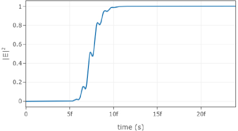
Figure 1: Record of at the center of the simulation space. This plot shows the time evolution of the squared electric field magnitude at the origin. Initially, the field magnitude is zero, indicating no electric field presence. As the simulation progresses, the electric field strength increases, exhibiting transient oscillations before stabilizing. After reaching the steady state (around 10 fs), the field magnitude remains constant at 1, confirming the successful generation of a circularly polarized plane wave. This verification step ensures that the wave retains its polarization characteristics throughout the simulation.
We then plotted the Lissajous figure, which is a projected harmonic-motion trace, for time steps ranging from 201 to 250. The result is shown in Fig. 2. One can observe that the projected trace does fit on the unit circle, indicating that the plane wave is circularly polarized. We calculate the average electric field intensity over this time frame and obtain a value of 0.9978, indicating an error of less than 1% compared to the unity radius reference.
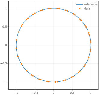
Figure 2: Lissajous figure for time steps ranging from 201 to 250, showing the projected traces fitting perfectly on the unit circle, indicating that the plane wave is circularly polarized. The reference circle and data points demonstrate the accuracy of the simulation.
Finally, the 2D electric field at the center of the domain is plotted for time steps ranging from 201 to 250. For the case where the source is , the result is displayed in Fig. 3 (a). Additionally, we modeled the case with , and the corresponding result is presented in Fig. 3 (b). As expected, the direction of polarization is reversed between these two cases, which confirms the expected behavior of the electric field under opposite phase shifts. The results clearly illustrate how the phase shift between the orthogonal components of the source influences the polarization direction of the resulting wave.
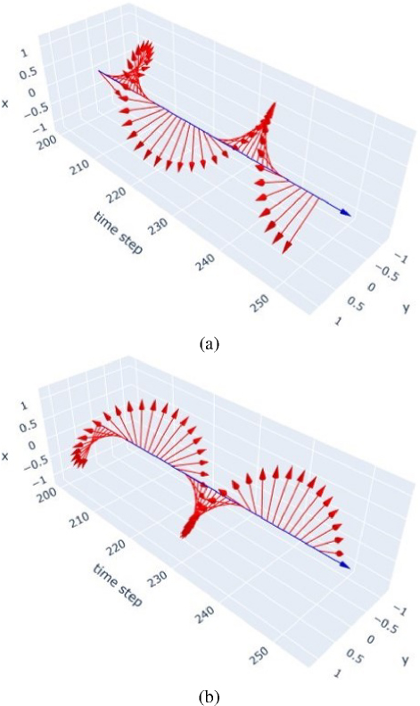
Figure 3: 2D electric field at the center of the simulation space for time steps ranging from 80 to 120: (a) the case where the source is , showing the electric field rotating from the positive y-axis toward the positive x-axis and (b) the case where the source is , with the electric field rotating from the negative y-axis toward the positive x-axis.
B. Broadband sources simulation
In the broadband simulation, a Gaussian pulse is used as the excitation:
| (12) |
where fs and fs.
Similar to Fig. 3, Fig. 4 shows the 2D electric field at the center of the simulation space for time steps ranging from 80 to 120, for the cases where the source is and . It can be observed that the Gaussian pulse exhibits a twist in both cases, but in opposite directions. In Fig. 4 (a), the electric field rotates from the positive y-axis toward the positive x-axis, while in Fig. 4 (b), the electric field rotates from the negative y-axis toward the positive x-axis.
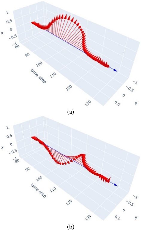
Figure 4: 2D electric field simulation results for time steps ranging from 80 to 120: (a) simulation with showing the expected circular polarization and (b) simulation with illustrating the reversed polarization direction. These results demonstrate the effectiveness of the TFSF technique in accurately modeling circularly polarized plane waves. The time evolution of the electric field is clearly depicted, highlighting the distinct polarization characteristics for each case.
It is also of particular interest to compute the axial ratio (AR) as a function of frequency. In ideal circular polarization, AR is exactly 1, indicating equal amplitude components in orthogonal directions. An increase in AR represents a deviation towards elliptical polarization, which can affect signal quality in communication systems. In these systems, maintaining low AR values is essential for minimizing cross-polarization and ensuring consistent signal reception. A shift in AR from 1 to 1.5 (which is normally the threshold value) represents an increasingly elliptical polarization, which can lead to a mismatch between the transmitted and received signals and reduce the effective power transferred to the receiver.
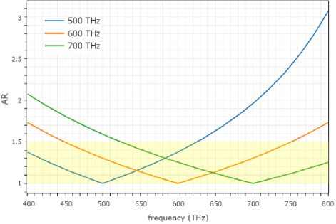
Figure 5: Axial ratio (AR) as a function of frequency for Gaussian pulses with center frequencies THz. AR is calculated using . At the center frequencies, AR equals 1, indicating circular polarization. As the frequency deviates from the center, AR increases, demonstrating a transition to elliptical polarization. For THz, AR remains below the threshold 1.5 over a total bandwidth of 300 THz.
In the second simulation, we retained the parameters of the Gaussian pulse as mentioned previously and tested various time shifts. The recorded electric field at the center is subjected to a discrete Fourier transform (DFT) across various frequencies, ranging from 300 THz to 800 THz with a spacing of 10 THz. After obtaining the frequency-domain field of the orthogonal components, AR is then calculated by dividing the length of the long axis by the length of the short axis , with:
| (13) |
| (14) |
where . By retaining the parameters of the Gaussian pulse, center frequencies s THz are tested with , and the results are shown in Fig. 5. It can be observed that at the center frequencies, the calculated AR values are equal to 1, indicating that the waves are circularly polarized. AR values gradually increase and become elliptically polarized as the frequency moves away from the center frequency. For THz, the total bandwidth where AR1.5 is 300 THz.
It is important to note that AR curves for broadband sources are independent of the waveform function and are solely determined by the factor , as analyzed in section 3B. The simulated results are consistent with the analytical predictions obtained using the Jones vector .
V. CONCLUSION
In this study, we have developed a comprehensive method for incorporating circular polarizations into time-domain EM simulations using the Fourier PSTD method. Our simulations verified the accuracy and stability of the proposed approach, as evidenced by the consistent field strength and accurate Lissajous figures. In addition to monochromatic sources, we also tested our method to accommodate broadband sources, such as Gaussian pulses, and analyzed AR across a wide frequency range. Analysis of AR demonstrated that while circular polarization is maintained at the center frequency, the polarization gradually transitions to elliptical as the frequency deviates from the center. This result is consistent with the expected behavior based on the frequency-dependent phase shift. Future work includes extending the polarization analysis from wave propagation to scattering in both simple and complexstructures.
REFERENCES
[1] Y. Lee, H. Kim, and C. Kim, “Rigorous optical modeling of circularly polarized light-emitting devices: Interaction of emitters with device geometries,” ACS Photonics, vol. 10, no. 9, pp. 3283-3290, 2023.
[2] L. Yan, Y. Li, V. Chandrasekar, H. Mortimer, J. Peltoniemi, and Y. Lin, “General review of optical polarization remote sensing,” International Journal of Remote Sensing, vol. 41, no. 13, pp. 4853-4864, 2020.
[3] B. Y. Toh, R. Cahill, and V. F. Fusco, “Understanding and measuring circular polarization,” IEEE Transactions on Education, vol. 46, no. 3, pp. 313-318, 2003.
[4] M. Sahal and V. Tiwari, “Review of circular polarization techniques for design of microstrip patch antenna,” in Proceedings of the International Conference on Recent Cognizance in Wireless Communication & Image Processing: ICRCWIP-2014, pp. 663-669, 2016.
[5] G. Bogdan, P. Bajurko, and Y. Yashchyshyn, “Time-modulated antenna array with dual-circular polarization,” IEEE Antennas and Wireless Propagation Letters, vol. 19, no. 11, pp. 1872-1875, Nov. 2020.
[6] J. Feng, Z. Yan, S. Yang, F. Fan, T. Zhang, X. Liu, X. Zhao, and Q. Chen, “Reflect-transmit-array antenna with independent dual circularly polarized beam control,” IEEE Antennas and Wireless Propagation Letters, vol. 22, no. 1, pp. 89-93, Jan.2023.
[7] R. Dutta, J. Ghosh, Z. Yang, and X. Zhang, “Multi-band multi-functional metasurface-based reflective polarization converter for linear and circular polarizations,” IEEE Access, vol. 9, pp. 152738-152748, 2021.
[8] N. Hussain, M.-J. Jeong, A. Abbas, T.-J. Kim, and N. Kim, “A metasurface-based low-profile wideband circularly polarized patch antenna for 5G millimeter-wave systems,” IEEE Access, vol. 8, pp. 22127-22135, 2020.
[9] S. Jiang and N. A. Kotov. “Circular polarized light emission in chiral inorganic nanomaterials,” Advanced Materials, vol. 35, no. 34, p. 2108431, 2023.
[10] A. Taflove and S. C. Hagness, Computational Electrodynamics: The Finite-Difference Time-Domain Method, 3rd ed. Norwood: Artech House,2005.
[11] A. Taflove, A. Oskooi, and S. G. Johnson, Advances in FDTD Computational Electrodynamics: Photonics and Nanotechnology. Norwood: Artech House, 2013.
[12] Q. H. Liu, “The PSTD algorithm: A time-domain method requiring only two cells per wavelength,” Microwave and Optical Technology Letters, vol. 15, no. 3, pp. 158-165, 1997.
[13] Q. H. Liu, “Large-scale simulations of electromagnetic and acoustic measurements using the pseudospectral time-domain (PSTD) algorithm,” IEEE Transactions on Geoscience and Remote Sensing, vol. 37, no. 2, pp. 917-926, 1999.
[14] J. W. Liu, Y.-S. Hsu, and S. H. Tseng, “Extracting field information embedded within a coarse pseudospectral time-domain simulation,” IEEE Antennas and Wireless Propagation Letters, vol. 17, no. 8, pp. 1488-1491, 2018.
[15] X. Gao, M. S. Mirotznik, and D. W. Prather, “A method for introducing soft sources in the PSTD algorithm,” IEEE Transactions on Antennas and Propagation, vol. 52, no. 7, pp. 1665-1671,2004.
BIOGRAPHIES

Jake W. Liu was born in Hualien, Taiwan, in 1995. He received the B.S. degree in Electrical Engineering from National Taiwan University, Taipei, Taiwan, in 2017, and the Ph.D. degree from Graduate Institute of Communication Engineering in 2022. His research interests include antenna measurement theory, calibration of phased array of antennas at millimeter wave frequencies, and computational electromagnetics. He is currently conducting his postdoctoral research at the Graduate Institute of Photonics and Optoelectronics, National Taiwan University.
ACES JOURNAL, Vol. 39, No. 12, 1035–1041
doi: 10.13052/2024.ACES.J.391201
© 2024 River Publishers