3-D Analytical Predictions of Surface-inset Axial Flux Machines with Different Halbach Arrangements

Youyuan Ni, Chenhao Liu, Benxian Xiao, and Yong Lin

School of Electrical Engineering & Automation
Hefei University of Technology, Hefei 230009, China
nyy@hfut.edu.cn, 2022110384@mail.hfut.edu.cn, xiaobenxian@hfut.edu.cn, linyong@hfut.edu.cn

Submitted On: September 24, 2024; Accepted On: January 14, 2025

ABSTRACT

A three-dimensional (3-D) analytical model with a high computational efficiency is proposed for a surface-inset axial flux machine (SIAFM). Accounting for the air-gap fringing field, the proposed 3-D analytical model is used to compute the magnetic field in the SIAFMs with conventional, Hat- and T-shaped Halbach arrangements. Based on the linear superposition method, the 3-D scalar potential equations for different regions with boundary condition equations are obtained. On this basis, the air-gap magnetic field and electromagnetic parameters can be derived. To demonstrate the advantages, the optimization performance of the T-shaped Halbach machine model is compared with that of conventional and Hat-shaped Halbach machine models. The prediction indicates that the optimized T-shaped Halbach machine model has the greatest electromagnetic torque. Finally, a 3-D finite element analysis (FEA) validates the 3-D analytical predictions.

Index Terms: 3-D analytical predictions, electromagnetic torque, finite element analysis, surface-inset axial flux machine, T-shaped Halbach arrangements.

I. INTRODUCTION

With the rapid development of various fields such as industrial automation, electric vehicles, and renewable energy utilization, the demand for efficient, compact, and high-performance machine drive systems is becoming increasingly urgent. Axial flux machines (AFMs) with their significant structural and performance advantages are gradually emerging among a wide variety of machine types. Table 1 shows their specific applications in the fields of new energy vehicles, aerospace, ship propulsion, and robotics [1, 2].

The topological structures of AFMs can be classified as single-stator single-rotor, double-stator single-rotor, single-stator double-rotor, and multiple-stator multiple-rotor [3]. Specifically, using multiple-stator and/or rotor in double-sided AFMs have been widely used in practice due to its ability to effectively reduce single-sided unbalanced magnetic force [11]. Compared to single-stator double-rotor AFMs, double-stator single-rotor AFMs can achieve an increase in torque through the magnetic fields interaction between the stators and provide significant advantages for the specific application areas with high performance requirement [12].

Table 1: Specific application of AFMs

Application Area	Specific Applications
New energy vehicles	Mercedes Vision 1-11 electric vehicle [4], McLaren new cars and other plug-in hybrid models [5]
Aerospace	The ”Spirit of Innovation” and Evolito [6, 7]
Ship propulsion	Propel D1 and Falcon electric outboard machines [8, 9]
Robots	Application of EMRAX188 AFMs in robots [10]

As one machine type, surface-inset axial flux machine (SIAFM) has the characteristics of compact structure, relatively high torque density and power-to-weight ratio [13]. With the advancement of technology, SIAFMs have shown broader application prospects in multiple fields. At present, due to complex production processes and high precision requirements for components, the manufacturing cost of SIAFMs is high, which limits their large-scale application. It is believed that in the near future, with the continuous maturity of technology and the reduction of costs, its application scope will continue to expand.

In recent years, researchers have shown great interest in the application of Halbach arrangements. Compared to those without Halbach arrangements, AFMs equipped with Halbach arrangements exhibit numerous attractive advantages. An AFM with multi-segment multipole ironless Halbach arrangements is investigated in [14]. In order to improve the torque density, a type of SIAFM with unequal thicknesses of Halbach arrangements is proposed in [15]. The combination of surface-inset and surface-mounted magnets for AFM is proposed in [16]. A novel SIAFM structure with radially layered magnets is investigated in [17]. It has the parallel excited radial Halbach arrangements and tangentially magnetized magnets, greatly improving the air-gap magnetic flux density performance. With the equal area of primary magnetic flux, the performance is enhanced by efficiently utilizing the internal space.

A three-dimensional (3-D) finite element analysis (FEA), as a solution of the magnetic fields of AFMs [18], takes a long time in both calculation and optimization processes. Instead, the analytical techniques are more suitable for predicting the performance of 3-D AFM models [19]. The method to convert a 3-D machine model to a linear machine can solve the two-dimensional (2-D) scalar magnetic potential equation and greatly reduce computational complexity [20]. A method with equivalence of solving the 2-D vector magnetic potential of a linear machine is proposed in [21, 22]. However, the existing 3-D analytical methods are still limited to solving the AFMs equipped with surface-mounted magnets and are incapable of analysis of the magnetic field in SIAFMs.

In this paper, a 3-D analytical model for SIAFM is proposed. Different from the 2-D radial flux machines, the air-gap fringing effect for SIAFMs needs to be considered. The 3-D analytical predictions are done for SIAFMs with three different Halbach arrangements. The stator slotting influence is considered by the Carter coefficient. The electromagnetic performances of slotted SIAFMs are analyzed, and the magnet parameters are optimized. In the case of equal magnet volume, the T-shaped Halbach optimized model exhibits significantly superior electromagnetic performance compared to the other models. Finally, a 3-D FEA model is utilized for the verification of the analytical prediction results. Thus, the 3-D model can effectively compute the magnetic field, with relatively high accuracy and modest time.

II. 3-D PHYSICAL MODEL OF SIAFM

Figure 1 shows three different segmented Halbach magnet arrangements for the rotor of SIAFMs. The conventional and Hat-shaped three-segment Halbach magnets are shown in Figs. 1 (a) and (b), respectively. The T-shaped three-segment Halbach magnets are shown in Fig. 1 (c).

Figure 2 shows the 3-D structure of a single-rotor dual-stator SIAFM with T-shaped Halbach magnets. The three-phase symmetric non-overlapping winding arrangement is utilized.

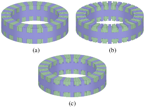
Figure 1: Three types of PM structures for SIAFMs: (a) conventional, (b) Hat-shaped Halbach magnets, and (c) T-shaped Halbach magnets.

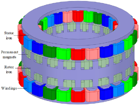
Figure 2: 3-D SIAFM structure with T-shaped Halbach magnets.

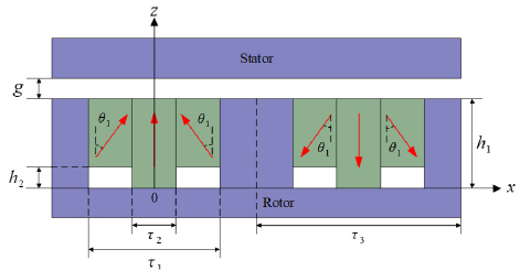
Figure 3: Parameters of T-shaped Halbach magnets.

Figure 3 provides the parameters of the T-shaped Halbach rotor model. h${}_{\mathrm{1}}$ is the axial length of the mid- magnet, h${}_{\mathrm{2}}$ is the difference between the side-magnet and mid-magnet in the axial length, g is the air-gap length, $\theta$${}_1$ is the magnetization angle of both symmetric side-magnets, and $\tau$${}_{\mathrm{1}}$ and $\tau$${}_2$ are the arc angles of the whole one-pole magnets and mid-magnets, respectively. $\tau$${}_3$ is the pole pitch. It is clearly seen that $\alpha$${}_1=$$\tau$${}_1$/$\tau$${}_3$ and $\alpha$${}_2=$$\tau$${}_2$/$\tau$${}_3$are the polar arc ratios. The analytical magnet domain is divided into two regions. One is the layer magnet region near the air-gap and the other is that far from the air-gap, as shown in Figs. 4 (a) and (b), respectively.

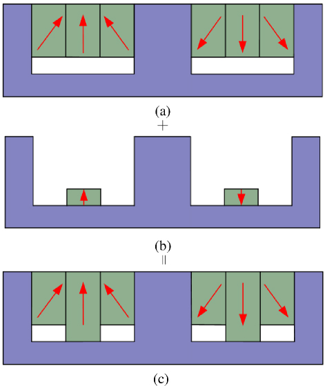
Figure 4: Linear superposition of T-shaped Halbach magnets: (a) layer magnets near air-gap, (b) layer magnets far from air-gap and (c) T-shaped Halbach magnets.

III. 3-D GENERAL SOLUTION EQUATIONS

Using the Cartesian coordinate system instead of the cylindrical one, the 3-D magnetic field distributions in SIAFMs are analyzed. In order to obtain high accuracy, the rotor is split into n${}_t$ (an odd number) hollow cylindrical pieces from inside to outside in the radial directions, with equal radial difference and unequal inner and outer radii. The average radius of the j-th cylindrical piece is denoted by:

$$R_j=R_1+(j-1)\frac{R_2-R_1}{n_t}+\frac{1}{2}\frac{R_2-R_1}{n_t},$$

(1)

where R${}_{\mathrm{1}}$ and R${}_{\mathrm{2}}$ are the inner and outer radii of rotor.

The initial spatial start point used for analytical calculation is chosen at x$\mathrm{=}$0 and z$\mathrm{=}$0. For the solution of 3-D field, general assumptions are necessary: the ideal linear demagnetization for magnets, the infinite magnetic permeability for the iron, and the ignored end effects for the windings. The relationship between the magnetic field intensity vector H and the scalar potential $\phi$ is:

$$\mathit{\text{H}}=-\mathrm{grad}\varphi .$$

(2)

The relationships between the flux density vector B and the magnetization vector M are:

$$\{\begin{array}{c}\mathit{\text{B}}={\mu }_0\mathit{\text{H}}\begin{array}{}\end{array}\begin{array}{}\end{array}\begin{array}{}\end{array}\begin{array}{}\end{array}\begin{array}{}\end{array}\begin{array}{}\end{array}\begin{array}{}\end{array}\begin{array}{}\end{array}\begin{array}{}\end{array}\begin{array}{}\end{array}\begin{array}{}\end{array}\begin{array}{}\end{array}\mathrm{in}\mathrm{the}\mathrm{air}\mathrm{region}\hfill \\ \mathit{\text{B}}={\mu }_0{\mu }_r\mathit{\text{H}}+{\mu }_0\mathit{\text{M}}\begin{array}{}\end{array}\mathit{\hspace{1em}\hspace{1em}}\mathrm{in}\mathrm{the}\mathrm{magnet}\mathrm{region}\hfill \end{array},$$

(3)

where $\mu$${}_0$ is vacuum permeability and $\mu$${}_r$ is magnet relative permeability.

For the linear 3-D analytical model, the principle of superposition is adopted. In order to achieve the general solutions of the scalar potential for 3-D Poisson or Laplace equations in each subdomain, the equations with the periodic symmetry are written as:

$$\{\begin{array}{c}{\varphi }_1^j(x,y,z)=-{\varphi }_1^j(x+\pi R_j/p,y,z)\hfill \\ {\varphi }_2^j(x,y,z)=-{\varphi }_2^j(x+{\alpha }_1\pi R_j/p,y,z)\hfill \\ {\varphi }_3^j(x,y,z)=-{\varphi }_3^j(x+{\alpha }_1\pi R_j/p,y,z)\hfill \\ {\varphi }_{1,2,3}^j(x,y,z)={\varphi }_{1,2,3}^j(x,y+2R_2-2R_1,z)\hfill \\ {\varphi }_1^j(x,y,h_1+g)={\varphi }_3^j(x,y,0)=0\hfill \end{array},$$

(4)

where p is the pole-pair number, $\phi$${}_1$${}^j$(x,y,z), $\phi$${}_2$${}^j$(x,y,z) and $\phi$${}_3$${}^j$(x,y,z) are the scalar magnetic potentials in the air-gap, the layer magnets near the air-gap and the layer magnets far from the air-gap, respectively.

A. 3-D air-gap governing equation

In the air-gap domain, the governing 3-D Laplace equation is expressed as:

$$\frac{{\partial }^2{\varphi }_1}{\partial r^2}+\frac{1}{r}\frac{\partial {\varphi }_1}{\partial r}+\frac{1}{r^2}\frac{{\partial }^2{\varphi }_1}{\partial {\theta }^2}+\frac{{\partial }^2{\varphi }_1}{\partial z^2}=0.$$

(5)

Adopting the technique of separating variables, according to (4), the 3-D analytical expression of (5) is:

${\varphi }_1^j$	$={\displaystyle \sum _{m=0}^{\mathrm{\infty }}}{\displaystyle \sum _{n=1,3\mathrm{\dots }}^{\mathrm{\infty }}}{A}_{{}_{1mn}}^j(e^{k_1^{j}z}-e^{2k_1^j{h}_1+2k_1^{j}g-k_1^{j}z})$
		$\times \cos ({\omega }_n^{j}x)\cos \{{\omega }_m^j\left[(y+(j-{\displaystyle \frac{n_t+1}{2}}){\displaystyle \frac{{}^{1}T_y}{n_t}}]\right\}$		(6)

where:

$$\{\begin{array}{c}{\omega }_n^j=np/R_j\hfill \\ {\omega }_m^j=m\pi /(R_2-R_1)\hfill \\ k_1^j=\sqrt{{\omega }_n^j{}^2+{\omega }_m^j{}^2}\hfill \end{array},$$

(7)

where A${}_{\mathrm{1}}$${}_{m\mathit{}n}$${}^j$ is the unknown coefficient, ${}^1$T${}_x$$\mathrm{=}$$\alpha$${}_{\mathrm{1}}$$\pi$R${}_j$/p and ${}^1$T${}_y$$\mathrm{=}$R${}_{\mathrm{2}}$$\mathrm{-}$R${}_{\mathrm{1}}$ are the half cycles of the j-th group of layer magnets near the air-gap in the x- and y-axis directions, respectively.

B. 3-D governing equation for layer magnets near the air-gap

For the layer magnets near the air-gap, during one electrical period, the expressions of 3-D components of the magnetization are:

$\{\begin{array}{c}{}^{1}M_x^j=(B_r/{\mu }_0)\sin ({\theta }_1)\hfill \\ {}^{1}M_y^j=0\hfill \\ {}^{1}M_z^j=(B_r/{\mu }_0)\cos ({\theta }_1)\hfill \end{array}\begin{array}{}\end{array}\begin{array}{c}\hfill {\displaystyle \frac{-{\alpha }_1\pi R_j}{2p}}\le x\le {\displaystyle \frac{-{\alpha }_2\pi R_j}{2p}}\hfill \\ \hfill h_2<z<h_1\hfill \end{array},$		(8)
$\{\begin{array}{c}{}^{1}M_x^j=0\hfill \\ {}^{1}M_y^j=0\hfill \\ {}^{1}M_z^j=B_r/{\mu }_0\hfill \end{array}\begin{array}{}\end{array}\begin{array}{c}\hfill {\displaystyle \frac{-{\alpha }_2\pi R_j}{2p}}\le x\le {\displaystyle \frac{{\alpha }_2\pi R_j}{2p}}\hfill \\ \hfill h_2<z<h_1\hfill \end{array},$		(9)
$\{\begin{array}{c}{}^{1}M_x^j=-(B_r/{\mu }_0)\sin ({\theta }_1)\hfill \\ {}^{1}M_y^j=0\hfill \\ {}^{1}M_z^j=(B_r/{\mu }_0)\cos ({\theta }_1)\hfill \end{array}\begin{array}{}\end{array}\begin{array}{c}\hfill {\displaystyle \frac{{\alpha }_2\pi R_j}{2p}}\le x\le {\displaystyle \frac{{\alpha }_1\pi R_j}{2p}}\hfill \\ \hfill h_2<z<h_1\hfill \end{array},$		(10)

Adopting double Fourier decomposition, the magnetizations in region S${}_1$ ($-$${}^1$T${}_x$/2$\le$x$\mathrm{\le }$3${}^1$T${}_x$/2, $-$${}^1$T${}_y$$\mathrm{\le }$y$\mathrm{\le }$${}^{\mathrm{1}}$T${}_y$) are written as:

$$\{\begin{array}{c}{}^{1}M_x^j=\sum _{m=0}^{\mathrm{\infty }}\sum _{i=1,3,5}^{\mathrm{\infty }}\left\{\begin{array}{c}{}^{1}M_{{}_{xmi}}^j\sin ({\omega }_i^{j}x)\hfill \\ \times \cos \{{\omega }_m^j\left[(y+(j-\frac{n_t+1}{2})\frac{{}^{1}T_y}{n_t}]\right\}\hfill \end{array}\right\}\hfill \\ {}^{1}M_y^j=0\hfill \\ {}^{1}M_z^j=\sum _{m=0}^{\mathrm{\infty }}\sum _{i=1,3,5}^{\mathrm{\infty }}\left\{\begin{array}{c}{}^{1}M_{{}_{zmi}}^j\cos ({\omega }_i^{j}x)\hfill \\ \times \cos \{{\omega }_m^j\left[(y+(j-\frac{n_t+1}{2})\frac{{}^{1}T_y}{n_t}]\right\}\hfill \end{array}\right\}\hfill \end{array},$$

(15)

During prediction of the magnetic field due to the layer magnets near the air-gap, the region of the layer magnets far from the air-gap is treated as a vacuum, as shown in Fig. 4 (a). The governing 3-D Poisson equation is:

$$\frac{{\partial }^2{\varphi }_2}{\partial r^2}+\frac{1}{r}\frac{\partial {\varphi }_2}{\partial r}+\frac{1}{r^2}\frac{{\partial }^2{\varphi }_2}{\partial {\theta }^2}+\frac{{\partial }^2{\varphi }_2}{\partial z^2}=\frac{1}{{\mu }_r}\mathrm{div}\mathit{\text{M}}.$$

(17)

Utilizing the technique of separating variables, according to (4), the 3-D analytical expression of (17) is:

$$\begin{array}{c}{\varphi }_2^j=\sum _{m=0}^{\mathrm{\infty }}\sum _{i=1,3\mathrm{\dots }}^{\mathrm{\infty }}\left[A_{{}_{2mi}}^j{e}^{k_2^{j}z}+B_{{}_{2mi}}^j{e}^{-k_2^{j}z}-\frac{{\omega }_i{}^j\cdot {}^{1}M_{xmi}^j}{{\mu }_{\mathrm{r}}{k}_2^j{}^2}\right]\hfill \\ \begin{array}{}\end{array}\times \cos ({\omega }_i^{j}x)\cos \{{\omega }_m^j\left[(y+(j-\frac{n_t+1}{2})\frac{{}^{1}T_y}{n_t}]\right\}\hfill \end{array},$$

(18)

where:

$$\{\begin{array}{c}{\omega }_i^j=ip/{\alpha }_1{R}_j\hfill \\ k_2^j=\sqrt{{\omega }_i^j{}^2+{\omega }_m^j{}^2}\hfill \end{array},$$

(19)

where A${}_{\mathrm{2}}$${}_{m\mathit{}i}$${}^j$ and B${}_{\mathrm{2}}$${}_{m\mathit{}i}$${}^j$ are the undetermined coefficients in the region of the layer magnets near the air-gap.

C. 3-D governing equation for layer magnets far from the air-gap

For the layer magnets far from the air-gap, in one electrical cycle, the expressions of 3-D components of magnetization are:

$\{\begin{array}{c}{}^{2}M_x^j=0\hfill \\ {}^{2}M_y^j=0\hfill \\ {}^{2}M_z^j=B_r/{\mu }_0\hfill \end{array}\begin{array}{}\end{array}\begin{array}{c}\hfill {\displaystyle \frac{-{\alpha }_2\pi R_j}{2p}}\le x\le {\displaystyle \frac{{\alpha }_2\pi R_j}{2p}}\hfill \\ \hfill 0<z<h_2\hfill \end{array},$		(20)
$\{\begin{array}{c}{}^{2}M_x^j=0\hfill \\ {}^{2}M_y^j=0\hfill \\ {}^{2}M_z^j=-B_r/{\mu }_0\hfill \end{array}\begin{array}{c}\hfill {\displaystyle \frac{2{\alpha }_1\pi R_j-{\alpha }_2\pi R_j}{2p}}\le x\le {\displaystyle \frac{2{\alpha }_1\pi R_j+{\alpha }_2\pi R_j}{2p}}\hfill \\ \hfill 0<z<h_2\hfill \end{array},$		(21)

where ${}^2$M${}_x$${}^j$, ${}^{\mathrm{2}}$M${}_y$${}^j$ and ${}^2$M${}_z$${}^j$ are the x, y and z-axis components of magnetization for the j-th group of layer magnets far from the air-gap, respectively.

Adopting the double Fourier decomposition, the magnetizations in region S${}_2$ ($-$${}^2$T${}_x$/2$\le$x$\le$3${}^2$T${}_x$/2, $-$${}^2$T${}_y$$\mathrm{\le }$y$\le$${}^2$T${}_y$) can be written as:

$$\{\begin{array}{c}{}^{2}M_x^j=0\hfill \\ {}^{2}M_y^j=0\hfill \\ {}^{2}M_z^j=\sum _{m=0}^{\mathrm{\infty }}\sum _{i=1,3,5}^{\mathrm{\infty }}{}^{2}M_{{}_{zmi}}^j\hfill \\ \begin{array}{cc}& \hfill \begin{array}{}\end{array}\hfill \end{array}\begin{array}{}\end{array}\times \cos ({\omega }_i^{j}x)\cos \{{\omega }_m^j\left[(y+(j-\frac{n_t+1}{2})\frac{{}^{2}T_y}{n_t}]\right\}\hfill \end{array},$$

(22)

where:

$$\{\begin{array}{c}{}^{2}M_{{}_{x0i}}^j={}^{2}M_{{}_{xmi}}^j=0\hfill \\ {}^{2}M_{{}_{z0i}}^j=\frac{1}{{}^{2}T_x\cdot {}^{2}T_y}{\int \int }_{S2}{}^{2}M_z^j\cos ({\omega }_i^{j}x)\mathrm{d}x\mathrm{dy}\hfill \\ {}^{2}M_{{}_{zmi}}^j=\frac{1}{{}^{2}T_x\cdot {}^{2}T_y}{\int \int }_{S2}{}^{2}M_z^j\cos ({\omega }_i^{j}x)\hfill \\ \begin{array}{}\end{array}\times \cos \{{\omega }_m^j\left[(y+(j-\frac{n_t+1}{2})\frac{{}^{2}T_y}{n_t}]\right\}\mathrm{d}x\mathrm{dy}\hfill \end{array},$$

(23)

where ${}^2$T${}_x$$\mathrm{=}$$\alpha$${}_{\mathrm{1}}$$\pi$R${}_j$/p and ${}^2$T${}_y$$\mathrm{=}$R${}_{\mathrm{2}}$-R${}_{\mathrm{1}}$ are the half cycles of the j-th group of layer magnets far from the air-gap in the x- and y-axis direction, respectively.

During prediction of the magnetic field due to the layer magnets far from the air-gap, the region of layer magnets near the air-gap is regarded as a vacuum. The governing 3-D Poisson equation is:

$$\frac{{\partial }^2{\varphi }_3}{\partial r^2}+\frac{1}{r}\frac{\partial {\varphi }_3}{\partial r}+\frac{1}{r^2}\frac{{\partial }^2{\varphi }_3}{\partial {\theta }^2}+\frac{{\partial }^2{\varphi }_3}{\partial z^2}=\frac{1}{{\mu }_r}\mathrm{div}\mathit{\text{M}}.$$

(24)

Using the technique of separating variables, according to (4), the 3-D analytical expression of (24) is:

$$\begin{array}{c}{\varphi }_3^j=\sum _{m=0}^{\mathrm{\infty }}\sum _{i=1,3\mathrm{\dots }}^{\mathrm{\infty }}{A}_{{}_{3mi}}^j(e^{k_2^{j}z}-e^{-k_2^{j}z})\cos ({\omega }_i^{j}x)\hfill \\ \begin{array}{}\end{array}\mathit{\hspace{1em}}\times \cos \{{\omega }_m^j\left[(y+(j-\frac{n_t+1}{2})\frac{{}^{2}T_y}{n_t}]\right\}\hfill \end{array},$$

(25)

where A${}_{\mathrm{3}}$${}_{m\mathit{}i}$${}^j$ is the undetermined coefficient in the region of the layer magnets far from the air-gap.

IV. SOLUTION OF COEFFICIENTS

There are four unknown coefficients A${}_{\mathrm{1}}$${}_{m\mathit{}n}$${}^j$, A${}_{\mathrm{2}}$${}_{m\mathit{}i}$${}^j$, B${}_{\mathrm{2}}$${}_{m\mathit{}i}$${}^j$ and A${}_{\mathrm{3}}$${}_{m\mathit{}i}$${}^j$ in the foregoing analytical equations. They need to be uniquely determined by the specific boundary conditions.

A. Boundary conditions at z$\mathrm{=}$h${}_{\mathrm{2}}$

At the boundary between different layer magnets (z$\mathrm{=}$h${}_{\mathrm{2}}$), the flux density and the magnetic field intensity are satisfied as:

$$\{\begin{array}{c}{{}^{2}B_{{}_z}^j(x,y,z)|}_{z=h_2}={{}^{3}B_{{}_z}^j(x,y,z)|}_{z=h_2}\hfill \\ {{}^{2}H_{{}_{x,y}}^j(x,y,z)|}_{z=h_2}={{}^{3}H_{{}_{x,y}}^j(x,y,z)|}_{z=h_2}\hfill \end{array},$$

(26)

where ${}^3$B${}_z$${}^j$(x,y,z) and ${}^3$H${}_{x\mathrm{,}y}$${}^j$(x,y,z) are the z-axis components of the flux density and the magnetic field intensity of the j-th group of layer magnets far from the air-gap, respectively.

According to (26), the relationship between the undetermined coefficients A${}_{\mathrm{2}}$${}_{m\mathit{}i}$${}^j$, B${}_{\mathrm{2}}$${}_{m\mathit{}i}$${}^j$, and A${}_{\mathrm{3}}$${}_{m\mathit{}i}$${}^j$ can be expressed as:

$$\{\begin{array}{c}{A}_{2mi}{}^j=\frac{[k_2({}^{1}M_{zmi}{}^j-{}^{2}M_{zmi}{}^j)+{\omega }_i{}^{1}M_{xmi}{}^j]e^{-k_2{h}_2}}{2{\mu }_r{k}_2{}^2}+A_{3mi}{}^j\hfill \\ B_{2mi}{}^j=\frac{[k_2({}^{1}M_{zmi}{}^j-{}^{2}M_{zmi}{}^j)-{\omega }_i{}^{1}M_{xmi}{}^j]e^{-k_2{h}_2}}{2{\mu }_r{k}_2{}^2}+A_{3mi}{}^j\hfill \end{array}.$$

(27)

B. Boundary conditions at z$\mathrm{=}$h${}_{\mathrm{1}}$

At the boundary between the air-gap and layer magnets near the air-gap (z$\mathrm{=}$h${}_{\mathrm{1}}$), the flux density and the magnetic field intensity are expressed as:

$$\{\begin{array}{c}{{}^{1}B_{{}_z}^j(x,y,z)|}_{z=h_1}={{}^{2}B_{{}_z}^j(x,y,z)|}_{z=h_1}\hfill \\ {{}^{1}H_{{}_{x,y}}^j(x,y,z)|}_{z=h_1}={{}^{2}H_{{}_{x,y}}^j(x,y,z)|}_{z=h_1}\hfill \end{array},$$

(28)

where ${}^1$H${}_{x\mathrm{,}y}$${}^j$(x,y,z) and ${}^1$B${}_z$${}^j$(x,y,z) are the z-axis components of the magnetic field intensity and the flux density in the air-gap domain. ${}^2$H${}_{x\mathrm{,}y}$${}^j$(x,y,z) and ${}^2$B${}_z$${}^j$(x,y,z) are the z-axis components of the magnetic field intensity and the flux density for the j-th group of magnets in the layer magnets near the air-gap, respectively.

According to (28), substituting (A.) and (18) into (2) and (3), the equations can be expressed as:

Accounting for the orthogonality of the trigonometric functions, from (27) and (29), a matrix equation can be constructed as:

$$\left[\begin{array}{cc}\hfill {\mathbf{C}}_{1m}^j\hfill & \hfill {\mathbf{C}}_{2m}^j\hfill \\ \hfill {\mathbf{F}}_{1m}^j\hfill & \hfill {\mathbf{F}}_{2m}^j\hfill \end{array}\right]\cdot \left[\begin{array}{c}\hfill {\mathbf{A}}_{1m}^j\hfill \\ \hfill {\mathbf{A}}_{3m}^j\hfill \end{array}\right]=\left[\begin{array}{c}\hfill {\mathbf{G}}_{1m}^j\hfill \\ \hfill {\mathbf{G}}_{2m}^j\hfill \end{array}\right],$$

(30)

where C${}_{\mathrm{1}}$${}_m$${}^j$ is a n$\mathrm{\times }$n matrix with m and n, C${}_{\mathrm{2}}$${}_m$${}^j$ is a n$\mathrm{\times }$i matrix with m, n and i, F${}_{\mathrm{1}}$${}_m$${}^j$ is a j$\mathrm{\times }$n matrix with m, n and i and F${}_{\mathrm{2}}$${}_m$${}^j$ is an i$\mathrm{\times }$i matrix with m and i.

By solution of (30), the unknown coefficients can be achieved. If the j-th group of magnets are calculated, the total magnetic flux density is the superposition of multiple groups of magnets and can be written as:

$$B_{\mathrm{res}}=\sum _{j=1}^{n_t}{B}^j.$$

(31)

V. 3-D ANALYTICAL PERFORMANCE OF SIAFM ACCOUNTING FOR SLOTTING AND AIR-GAP FRINGING EFFECT

The slotless flux density B${}_z$ at h${}_{\mathrm{1}}$+g in the z-axis direction can be written as:

$$\begin{array}{c}{B_z|}_{h_1+g}=-2{\mu }_0\sum _{j=1}^{n_t}\sum _{m=0}^{\mathrm{\infty }}\sum _{n=1,3}^{\mathrm{\infty }}{A}_{{}_{1mn}}^j{k}_1^j{e}^{k_1^j(h_1+g)}\hfill \\ \begin{array}{}\end{array}\begin{array}{}\end{array}\mathit{\hspace{1em}}\cos ({\omega }_n^{j}x)\times \cos \{{\omega }_m^j\left[(y+(j-\frac{n_t+1}{2})\frac{{}^{1}T_y}{n_t}]\right\}\hfill \end{array}.$$

(32)

In order to compute the magnetic field in the slotted SIAFMs, the slotting effect needs to be considered. Thus, the Carter’s coefficient method is utilized. This method uses several equivalent air-gap lengths instead of the actual relatively complex air-gap distributions [23].

According to the analytically derived slotless magnetic field, the coefficient with the equivalent air-gap length is given as:

$$C_s^{\prime }=\{\begin{array}{cc}{C}_s\hfill & \hfill (\left(R_2+R_1\right)/2N_s-n_s,\pi \left(R_2+R_1\right)/2N_s+n_s)\hfill \\ 1\hfill & \hfill \text{others}\hfill \end{array},$$

(33)

where C${}_s$ is Carter’s coefficient, N${}_s$ is the slot number and n${}_s$ is the circumferential length of half one slot.

By Fourier decomposition of Carter coefficient in one period, the coefficient is written as:

The flux density in the air-gap of the slotted SIAFM can be expressed as:

$$B_{\mathrm{slotted}}=\frac{B_{\mathrm{res}}}{C_s^{\prime }}.$$

(36)

Because of the continuous magnetic circuit, there exists a magnetic field outside the air-gap and iron in the 3-D space. This is named the air-gap fringing effect. For high computation accuracy, the air-gap fringing effect cannot be ignored and needs to be considered. The air-gap fringing magnetic field is shown in Fig. 5. The air-gap fringing field coefficient is defined as:

$$C_{\mathrm{fr}}=1+\frac{\pi (2|y|-{}^{1}T_y)}{4g}.$$

(37)

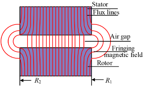
Figure 5: Air-gap fringing magnetic field in 3-D model.

Thus, the slotted flux density in the z-axis direction can be written as:

${B_z|}_{h_1+g}^{{}^{\prime }}=$
$\{\begin{array}{c}\hfill {\displaystyle \frac{{B_z|}_{h_1+g}}{C_s{C}_{\mathrm{fr}}}}\begin{array}{}\end{array}\{\begin{array}{c}\beta -{\alpha }_{cp}{R}_j/2\le x\le \beta -{\alpha }_{cp}{R}_j/2+n_s\begin{array}{}\end{array}\hfill \\ -{}^{1}T_y\le y\le -{}^{1}T_y/2\begin{array}{c}\hfill \mathrm{or}{}^{1}T_y/2\le y\le {}^{1}T_y\hfill \end{array}\hfill \end{array}\hfill \\ \hfill {\displaystyle \frac{{B_z|}_{h_1+g}}{C_{\mathrm{fr}}}}\begin{array}{}\end{array}\{\begin{array}{c}\beta -{\alpha }_{cp}{R}_j/2+n_s\le x\le \beta +{\alpha }_{cp}{R}_j/2-n_s\hfill \\ -{}^{1}T_y\le y\le -{}^{1}T_y/2\begin{array}{c}\hfill \mathrm{or}{}^{1}T_y/2\le y\le {}^{1}T_y\hfill \end{array}\hfill \end{array}\hfill \\ \hfill {\displaystyle \frac{{B_z|}_{h_1+g}}{C_s{C}_{\mathrm{fr}}}}\begin{array}{}\end{array}\{\begin{array}{c}\beta +{\alpha }_{cp}{R}_j/2-n_s\le x\le \beta +{\alpha }_{cp}{R}_j/2\begin{array}{}\end{array}\hfill \\ -{}^{1}T_y\le y\le -{}^{1}T_y/2\begin{array}{c}\hfill \mathrm{or}{}^{1}T_y/2\le y\le {}^{1}T_y\hfill \end{array}\hfill \end{array}\hfill \\ \hfill \begin{array}{c}\hfill {\displaystyle \frac{{B_z|}_{h_1+g}}{C_s}}\begin{array}{}\end{array}\{\begin{array}{c}\beta -{\alpha }_{cp}{R}_j/2\le x\le \beta -{\alpha }_{cp}{R}_j/2+n_s\begin{array}{}\end{array}\hfill \\ -{}^{1}T_y/2\le y\le {}^{1}T_y/2\hfill \end{array}\hfill \\ \hfill {B_z|}_{h_1+g}\begin{array}{}\end{array}\{\begin{array}{c}\beta -{\alpha }_{cp}{R}_j/2+n_s\le x\le \beta +{\alpha }_{cp}{R}_j/2-n_s\hfill \\ -{}^{1}T_y/2\le y\le {}^{1}T_y/2\hfill \end{array}\hfill \\ \hfill {\displaystyle \frac{{B_z|}_{h_1+g}}{C_s}}\begin{array}{}\end{array}P\{\begin{array}{c}\beta +{\alpha }_{cp}{R}_j/2-n_s\le x\le \beta +{\alpha }_{cp}{R}_j/2\begin{array}{}\end{array}\hfill \\ -{}^{1}T_y/2\le y\le {}^{1}T_y/2\hfill \end{array}\hfill \end{array}\hfill \end{array},$		(38)

where:

$$\beta =R_j[-{\omega }_{r}t+{\alpha }_{cp}(s-1)],$$

(39)

where $\omega$${}_r$ is the angular speed, $\alpha$${}_{cp}$ is the coil pitch angle and s denotes the s-th slot.

The flux linkage of one coil is:

$$\mathrm{\Psi }={N\underset{{\mathrm{S}}_3}{\iint }{B}_{\mathrm{z}}|}_{h_1+g}^{\prime }\mathrm{d}S,$$

(40)

where N is the number of coil turns. The scope of S${}_3$ is $\beta$$-$$\alpha$${}_{cp}$R${}_j$/2$\le$x$\mathrm{\le }$$\beta$+$\alpha$${}_{cp}$R${}_j$/2 and $-$${}^1$T${}_y$$\mathrm{\le }$y$\mathrm{\le }$${}^{\mathrm{1}}$T${}_y$.

The back electromotive force (EMF) for the s-th coil is expressed as:

$$W_2=\{\begin{array}{cc}{}^{1}T_y+\frac{4g}{\pi }\ln \left(1+\frac{\pi {}^{1}T_y}{4g}\right)\hfill & m=0\hfill \\ \frac{2\sin ({\omega }_m{}^{1}T_y/2)}{{\omega }_m}\hfill & \\ \cos \left[{\omega }_m\left(j-\frac{n_t+1}{2}\right){}^{1}T_y\right]\hfill & \\ +{\int }_{-{}^{1}T_y}^{-{}^{1}T_y/2}\frac{1}{C_{\text{fr}}}\hfill & \\ \cos \left\{{\omega }_m\left[y+\left(j-\frac{n_t+1}{2}\right)\frac{{}^{1}T_y}{n_t}\right]\right\}dy\hfill & \\ +{\int }_{{}^{1}T_y/2}^{{}^{1}T_y}\frac{1}{C_{\text{fr}}}\hfill & \\ \cos \left\{{\omega }_m\left[y+\left(j-\frac{n_t+1}{2}\right)\frac{{}^{1}T_y}{n_t}\right]\right\}dy\hfill & m\ne 0\hfill \end{array}.$$

(43)

The analytical calculation formula for the electromagnetic torque is:

$$T_e=\frac{e_A{i}_A+e_B{i}_B+e_C{i}_C}{{\omega }_r},$$

(44)

where i${}_a$, i${}_b$ and i${}_c$ are the three-phase currents.

VI. 3-D ANALYTICAL COMPARSION AND VERIFICATION

Using the given 3-D analytical equations, the performances of the SIAFM with T-shaped segmented Halbach magnets can be predicted. Table 2 presents its main parameters. The performances of the SIAFMs for conventional and Hat-shaped three-segment Halbach magnets are also investigated for comparison. It is noted that all SIAFMs have the same magnet usage.

For the SIAFM with T-shaped magnets, the polar-arc ratio $\alpha$${}_2$ and the magnetization angle $\theta$${}_1$ are chosen as two optimization variables. The single optimization objective is to maximize the electromagnetic torque. Figure 6 shows the 3-D analytical average electromagnetic torque with $\theta$${}_1$ and $\alpha$${}_2$. It is derived that the optimal variables are $\theta$${}_1=$55${}^{\circ }$ and $\alpha$${}_2=$0.27.

A 3-D FEA model is used for verification. The input parameters include the geometric dimensions and material properties and the three-phase currents. The applied boundary conditions are that the scalar potentials on all the outer surfaces are set to zero for the whole 3-D cylindrical solution region.

Table 2: SIAFM model parameters

Symbol	Parameter	Value
p/Q	Numbers of poles/slots	20/24
B${}_r$(T)	Magnet remanence	1.1
$\mu$${}_r$	Magnet relative permeability	1.05
N	Number of turns of one coil	16
R${}_{\mathrm{1}}$/R${}_{\mathrm{2}}$(mm)	Inner/outer radii of rotor	25/35
g (mm)	Air-gap length	1
$\alpha$${}_1$	Pole-arc ratio	0.67
L (mm)	Machine axial length	30
J (A/mm${}^2$)	Current density	6.37
n (r/min)	Rated rotational speed	3000

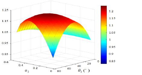
Figure 6: 3-D analytical electromagnetic torque with variables for T-shaped Halbach magnets.

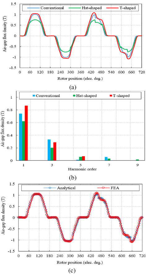
Figure 7: Comparison of air-gap flux density waveforms: (a) 3-D analytical predictions of flux density waveforms for three different SIAFMs, (b) flux density waveform harmonics for three SIAFMs and (c) two flux density waveforms for optimized T-shaped Halbach magnets from 3-D analytical and FEA models.

Table 3: Air-gap flux densities of three SIAFMs

	Conventional	Hat-shaped	T-shaped
Fundamental	0.74 T	0.62 T	0.87 T
THD	45.51%	34.69%	34.52%

Figure 7 (a) compares the 3-D analytically predicted air-gap flux density waveforms for three SIAFMs. Figure 7 (b) presents the main harmonic comparison corresponding to their air-gap flux density waveforms of three SIAFMs. Table 3 lists the air-gap flux density comparison. It is obviously seen that the T-shaped Halbach magnets has the best waveform. Figure 7 (c) compares the air-gap flux density waveforms of optimized T-shaped Halbach magnets from 3-D analytical and FEA models. It can be clearly observed that the two waveforms match well.

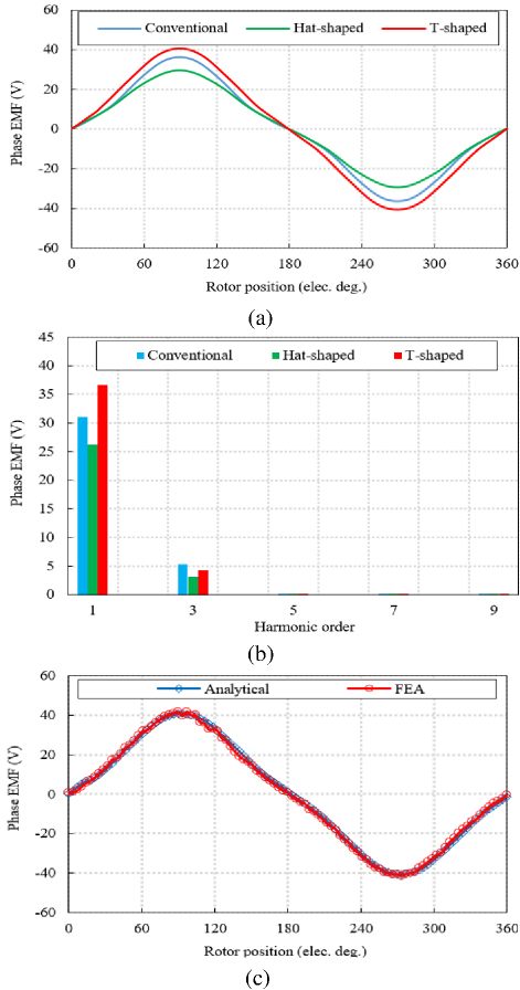
Figure 8: Comparison of back-EMF waveforms: (a) 3-D analytical predictions of back-EMF waveforms for three different SIAFMs, (b) back-EMF waveform harmonics for three SIAFMs and (c) two back-EMF waveforms for optimized T-shaped Halbach magnets from 3-D analytical and FEA models.

Figure 8 (a) presents the comparison of phase back-EMF waveforms for three different SIAFMs. Figure 8 (b) shows the main harmonic comparison corresponding to their phase back-EMF waveforms of three SIAFMs. Table 4 lists the back-EMF value comparison. It is obviously seen that the T-shaped Halbach magnet has the best waveform. The two phase back-EMF waveforms of the optimized T-shaped Halbach magnets from 3-D analytical and FEA methods show excellent consistency, as presented in Fig. 8 (c).

Table 4: Back-EMFs of three SIAFMs

	Conventional	Hat-shaped	T-shaped
Fundamental	31.02 V	26.23 V	36.53 V
THD	17.12%	12.33%	11.63%

Electromagnetic torque is an important machine operation performance. Figure 9 (a) presents the three electromagnetic torque waveforms for the compared SIAFMs. Table 5 lists the electromagnetic torque value comparison. It can be observed that the T-shaped Halbach arrangement has the largest fundamental and ripple values. The reason for the largest ripple value is interesting. For the T-shaped Halbach arrangement, although the 3rd harmonic of each-phase back-EMF is the lowest, according to (44), the resultant electromagnetic torque generated by all integer multiples of the 3rd harmonics of three-phase back-EMFs multiplied by the fundamental component of three-phase currents is zero. In addition, the two torque waveforms for the optimized T-shaped Halbach magnets obtained from 3-D analytical and FEA models show excellent agreement, as presented in Figure 9 (b).

In addition, the amplitude of the reluctance torque of the three compared machines is less than 1.1 mNm. It can be ignored compared to the electromagnetic torque. Thus, the reluctance torque waveform is not presented.

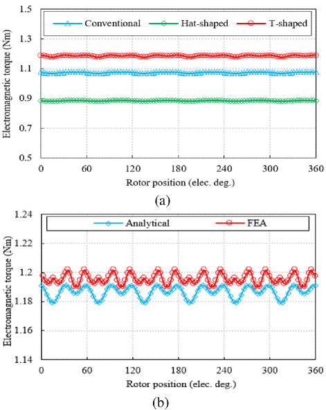
Figure 9: Comparison of torque waveforms: (a) three torque waveforms of three different SIAFMs and (b) two torque waveforms of optimized T-shaped Halbach magnets from 3-D analytical and FEA models.

Table 5: Electromagnetic torques of three SIAFMs

	Conventional	Hat-shaped	T- shaped
Average	1.075 Nm	0.885 Nm	1.187 Nm
Ripple	0.0103%	0.00654%	0.0122%

For actual industrial applications, the nonlinearity of the iron core of machines usually needs to be considered. Different from linear magnetic permeability,the magnetic field can be determined through the relatively complex iteration solution process with setting a convergence value. Compared with the linear SIAFM model, the flux density value of nonlinear SIAFM model is low. Thus, due to the saturation effect, the EMF and electromagnetic torque values of nonlinear SIAFM are lower than those of corresponding linear SIAFM. The specific numerical value depends on the saturation level.

VII. CONCLUSION

Different from the 2-D radial flux machines, it is necessary to consider the air-gap fringing effect for SIAFMs. Using the proposed 3-D linear analytical model for SIAFMs, with the principle of linear superposition, analysis of the 3-D magnetic field is made for SIAFMs with T-shaped Halbach magnets, taking into account the edge effects of the rotor. In addition, the two parameters of the Halbach magnets are selected as the optimization variables to optimize the electromagnetic torque. With equal consumption of permanent magnets, compared with the SIAFM models with conventional and Hat-shaped Halbach magnets, the SIAFM with optimized T-shaped Halbach magnets has the best air-gap flux density and back-EMF, and the largest electromagnetic torque. FEA results verify the correctness of the 3-D analytical and optimization model with T-shaped Halbach magnets.

For computational electromagnetics, firstly, computation time is of great significance. The proposed 3-D analytical model can solve and optimize the magnetic field in much less time than the 3-D FEA model. In other words, the proposed model has very high computational efficiency. Secondly, computation accuracy is of equal importance. It is known that the FEA model has high computation accuracy with enough mesh. Based on Maxwell’s equations, the proposed model can exhibit high accuracy. Finally, the proposed 3-D analytical model can show clearly the relationships between different physical variables. These advantages are very useful for design and development of novel machines for industrial applications.

In future work, other performances of this kind of machines with different magnet configurations will be investigated. Based on electromagnetic computation, thermal optimization solutions and advanced cooling techniques to ensure operational stability in high-torque applications will be explored. These in-depth explorations not only reflect the foundational significance of the existing work but also offer a perspective on the evolutionary potential of research in this area.

REFERENCES

[1] S. Kumar, W. Zhao, Z. S. Du, T. A. Lipo, and B. Kwon, “Design of ultrahigh speed axial-flux permanent magnet machine with sinusoidal back EMF for energy storage application,” IEEE Trans. Magn., vol. 51, no. 11, pp. 1-4, Nov. 2015.

[2] J. Zhu, G. H. Li, D. Cao, Z. Y. Zhang, and S. H. Li, “Comparative analysis of coreless axial flux permanent magnet synchronous generator for wind power generation,” J. Electr. Eng. Technol., vol. 15, pp. 727-735, 2020.

[3] F. Nishanth, J. Van Verdeghem, and E. L. Severson, “A review of axial flux permanent magnet machine technology,” IEEE Trans. Ind. Appl., vol. 59, no. 4, pp. 3920-3933, 2023.

[4] Electrek, Mercedes-Benz Unveils Vision One Eleven Concept with Axial Flux Motors and ‘Unique Battery Chemistry’ [Online]. Available: https://electrek.co/2023/06/15/mercedes-benz-vision-one-eleven-concept-axial-flux-motors-ev-electric/

[5] McLaren, Artura Coupe [Online]. Available: https://cars.mclaren.com/us-en/artura

[6] Evolito, ACCEL: The World’s Fastest Electric Plane [Online]. Available: https://evolito.aero/accel/

[7] Evolito, Axial flux motors [Online]. Available: https://evolito.aero/axial-flux-motors/

[8] Propel, D1 [Online]. Available: https://propel.me/d1/

[9] EPTechnologies, Falcon electric outboard launch [Online]. Available: https://www.metstrade.com/exhibitors/eptechnologies/news/falcon-electric-outboard-launch

[10] EMRAX, EMRAX 188 [Online] https://emrax.com/e-motors/emrax-188/

[11] W. L. Soong, Z. Cao, E. Roshandel, and S. Kahourzade, “Unbalanced axial forces in axial-flux machines,” in 32nd Australasian Universities Power Engineering Conference, pp. 1-6, 2022.

[12] S. Ge, W. Geng, and Q. Li, “A new flux-concentrating rotor of double stator and single rotor axial flux permanent magnet motor for electric vehicle traction application,” in 2022 IEEE Vehicle Power and Propulsion Conference, pp. 1-6, 2022.

[13] S. Amin, S. Khan, and S. S. Hussain Bukhari, “A comprehensive review on axial flux machines and its applications,” in 2nd International Conference on Computing, Mathematics and Engineering Technologies, Sukkur, Pakistan, pp. 1-7, 2019.

[14] T. Okita and H. Harada, “3-D analytical model of axial-flux permanent magnet machine with segmented multipole-Halbach array,” IEEE Access, vol. 11, pp. 2078-2091, 2023.

[15] L. Yang, K. Yang, S. J. Sun, Y. X. Luo, and C. Luo, “Study on the influence of a combined-Halbach array for the axial flux permanent magnet electrical machine with yokeless and segmented armature,” IEEE Trans. Magn., vol. 60, no. 3, pp. 1-5, Mar. 2024.

[16] Y. Cao, L. Feng, R. Mao, and K. Li, “Analysis of analytical magnetic field and flux regulation characteristics of axial-flux permanent magnet memory machine,” IEEE Trans. Magn., vol. 58, no. 9, pp. 1-9, Sep. 2022.

[17] X. Wang, X. Zhao, P. Gao, and T. Li, “A new parallel magnetic circuit axial flux permanent magnet in-wheel motor,” in 24th International Conference on Electrical Machines and Systems, pp. 1107-1111, 2021.

[18] W. Geng and Z. Zhang, “Analysis and implementation of new ironless stator axial-flux permanent magnet machine with concentrated nonoverlapping windings,” IEEE Trans. Energy Convers., vol. 33, no. 3, pp. 1274-1284, Sep. 2018.

[19] A. Zerioul, L. Hadjout, Y. Ouazir, H. Bensaidane, A. Benbekai, and O. Chaouch, “3D analytical model to compute the electromagnetic torque of axial flux magnetic coupler with a rectangular-shaped magnet,” in International Conference on Electrical Sciences and Technologies in Maghreb, pp. 1-4, 2018.

[20] B. Dolisy, S. Mezani, T. Lubin, and J. Lévêque, “A new analytical torque formula for axial field permanent magnets coupling,” IEEE Trans. Energy Conver., vol. 30, no. 3, pp. 892-899, Sep. 2015.

[21] W. Xu, Y. Hu, Y. Zhang, and J. Wang, “Design of an integrated magnetorheological fluid brake axial flux permanent magnet machine,” IEEE Trans. Transp. Electr., vol. 10, no. 1, pp. 1876-1886, Mar. 2024.

[22] A. Hemeida and P. Sergeant, “Analytical modeling of surface PMSM using a combined solution of Maxwell’s equations and magnetic equivalent circuit,” IEEE Trans. Magn., vol. 50, no. 12, pp. 1-13, Dec. 2014.

[23] O. Laldin, S. D. Sudhoff, and S. Pekarek, “Modified Carter’s coefficient,” IEEE Trans. Energy Conver., vol. 30, no. 3, pp. 1133-1134, Sep. 2015.

BIOGRAPHIES

Youyuan Ni received the B.Eng. and Ph.D. degrees in electrical engineering from the Hefei University of Technology, Hefei, China, in 1999 and 2006, respectively. Since 2006, he has been with Hefei University of Technology, where he is currently an associate professor. His current research interest includes design and control of electric machines.

Chenhao Liu received the B.Eng. degree in electrical engineering and automation from Liaoning Technical University, Huludao, China, in 2021. He is currently working toward the M.E. degree in electrical engineering with Hefei University of Technology. His current research interests include design of permanent magnet machines.

Benxian Xiao received the Ph.D. degree from the Department of Automation, School of Electrical Engineering & Automation, Hefei University of Technology, Hefei, China, in 2004. He is currently a Professor of control theory and control engineering subjects. His current research interests include fault diagnosis, fault-tolerant control, intelligent control, automotive steering control systems, and system modeling and simulation.

Yong Lin received the B.Eng. and M.S. degrees from Hefei University of Technology, Hefei, China, in 1995 and 2002, both in automation engineering. He is currently an associate researcher. His research interests include automotive control systems and system modeling and simulation.

ACES JOURNAL, Vol. 40, No. 1, 79–88
doi: 10.13052/2025.ACES.J.4001010
© 2025 River Publishers

ABSTRACT

I. INTRODUCTION

II. 3-D PHYSICAL MODEL OF SIAFM

III. 3-D GENERAL SOLUTION EQUATIONS

A. 3-D air-gap governing equation

B. 3-D governing equation for layer magnets near the air-gap

C. 3-D governing equation for layer magnets far from the air-gap

IV. SOLUTION OF COEFFICIENTS

V. 3-D ANALYTICAL PERFORMANCE OF SIAFM ACCOUNTING FOR SLOTTING AND AIR-GAP FRINGING EFFECT

VI. 3-D ANALYTICAL COMPARSION AND VERIFICATION

VII. CONCLUSION

REFERENCES

BIOGRAPHIES