Analysis of Induction-polarization Response Characteristics of Marine Controlled-source Electromagnetic Multiphase Composite Medium

Chunying Gu${}^{\mathbf{\text{1}}}$, Suyi Li${}^{\mathbf{\text{1}}}$, and Silun Peng${}^{\mathbf{\text{2*}}}$

¹College of Instrumentation and Electrical Engineering
Jilin University, Changchun 130061, China
cygu20@mails.jlu.edu.cn, lsy@jlu.edu.cn

²College of Automotive Engineering
Jilin University, Changchun 130022, China
${}^{*}$pengsilun@jlu.edu.cn

Submitted On: September 25, 2024; Accepted On: January 10, 2025

ABSTRACT

The complex composition and structure of the submarine reservoir and its secondary pyrite, which are multiphase composite media, can provoke the induced polarization (IP) effect, resulting in the change of the marine controlled-source electromagnetic (CSEM) induction-polarization response, which directly affects geological interpretation results. In this paper, the generalized effective-medium theory of induced polarization (GEMTIP) model is introduced to study the influence of composition, structure and geometric characteristics of submarine reservoirs and secondary pyrite on the 3D marine CSEM induction-polarization response. We first construct the 3D finite-difference frequency-domain (FDFD) electromagnetic field governing equation based on the GEMTIP model, apply the emission source on the non-uniform grid, and solve the linear equations by using the difference coefficient matrix. Then we perform forward calculation on a typical 1D reservoir model to verify the correctness and effectiveness of the proposed algorithm. Finally, we design the reservoir and secondary pyrite models, and analyze the influence laws of IP parameters and polarization layer geometry parameters on the 3D marine CSEM induction-polarization response. These studies are of great value for understanding the relationship between submarine multiphase composite medium and electromagnetic wavepropagation.

Index Terms: GEMTIP model, induced polarization (IP) effect, marine controlled-source electromagnetic (CSEM), reservoir polarization, secondary pyrite polarization.

I. INTRODUCTION

The marine controlled-source electromagnetic (CSEM) method has become an important geophysical method for deep-sea oil exploration, seabed geological structure investigation and marine ecological environment survey due to its advantages of high precision, low cost and wide range [1–7]. In the actual exploration of marine CSEM, multiphase composite media such as submarine oil reservoir and its secondary pyrite are often accompanied by the induced polarization (IP) effect [8–11], that is, under the action of applied electric field, positive and negative charges in the subsea multiphase composite medium will move in a directional way and accumulate to form double electric layers on both sides of the interface. After the applied electric field is turned off, positive and negative charges will return to the original state, thus forming a displacement current in the opposite direction of the applied electric field. This phenomenon will directly affect the measurement results of induction-polarization response of marine CSEM. Therefore, it is necessary to study the IP effect simulation of marine CSEM multiphase composite medium for improving the accuracy of geological interpretation of exploration data.

In recent years, some progress has been made in the simulation of the IP effect of marine CSEM. Wang et al. [12] established two 1D polarized medium models of reservoir generating IP effect based on the Cole-Cole model and analyzed the influence of IP parameters of the two models on electromagnetic response. Huang [13] calculated the 1D marine CSEM electromagnetic response with IP effect and analyzed the influence degree of different Cole-Cole model parameters on the response. Liu et al. [14] combined electromagnetic induction and IP effect, used real resistivity and complex resistivity (Cole-Cole) models to calculate the 1D CSEM response, and evaluated the influence of noise level on electromagnetic response and IP effect on inversion. Ding et al. [15] calculated the 1D and 2D marine CSEM response by introducing the Cole-Cole model and studied the influence of IP effect on marine CSEM response. Mittet [16] conducted induction-polarization dual-field forward modeling based on the fictitious wave domain method, calculated the electromagnetic response of marine CSEM, and analyzed the influence of IP parameters in the Cole-Cole model on the electromagnetic response. Xu and Sun [17] designed polarized medium models with different field source azimuths, IP parameters and terrain, implemented 2.5D marine CSEM forward modeling based on adaptive finite element method, and analyzed the influence law of Cole-Cole model parameters on electromagnetic response. Li et al. [18] realized finite volume forward modeling of marine CSEM in 3D frequency domain based on the Cole-Cole model and applied dual-frequency IP phase decoupling technology to marine CSEM data interpretation, which improved the sensitivity of the IP phase to polarized reservoir objects. Qiu et al. [19] used the integral equation method to conduct a 3D forward modeling of marine CSEM with IP effect, adopted the scattering and superposition methods to calculate the dyadic Green’s function, studied the response rule of the Cole-Cole polarization model, and analyzed the influence law of various model parameters. At present, although good research results have been obtained, the Cole-Cole model in the above marine CSEM forward modeling is only a qualitative description, lacking the physical and geometric characteristics of relevant actual petrology, so it cannot directly explain how the structure and mineral composition of rocks or reservoirs affect the conductive properties of rocks. Therefore, it is of great significance to find a physical model that can relate the conductivity characteristics of the seafloor strata to its structure, composition and polarizability, and study the influence law of the model parameters on the marine CSEM field to improve the interpretation accuracy of later data.

The generalized effective-medium theory of induced polarization (GEMTIP) model is a unified mathematical-physical model based on effective-medium theory (EMT), IP theory and Born approximation principle for heterogeneity, multiphase structure and polarizability of rock or reservoir [20–22]. The model is derived strictly based on Maxwell’s equation of multiphase composite conductive medium, including both surface and volume polarization effects, and is suitable for describing electrode polarization effects related to electron polarization and thin film polarization effects related to ion polarization [23–25]. IP parameters of the GEMTIP model (such as matrix conductivity, volume fraction, relaxation parameters, grain radius, etc.) have clear physical definitions and are closely related to the reservoir structure, mineral grain size, shape, polarization, porosity and other geometric-physical properties, which can better describe the IP response characteristics of the reservoir. This provides a quantitative analysis method for studying the conductivity characteristics of multiphase composite reservoirs [26, 27].

In this paper, the GEMTIP composite conductivity model is introduced to analyze the influence of composition, structure and geometric characteristics of submarine reservoir and secondary pyrite on the induction-polarization response of marine CSEM. First, based on Maxwell’s equation and GEMTIP model, a 3D finite difference electromagnetic field governing equation in frequency domain is established. After completing the non-uniform mesh generation and the emission source layout, the linear equations are solved directly by using the difference operator matrix. The correctness and effectiveness of the algorithm are verified by the forward calculation of a typical 1D reservoir model. Finally, we build the reservoir and secondary pyrite models and perform numerical calculations to study the influence characteristics of GEMTIP model parameters on the marine CSEM field response, and to analyze the influence rules of geometry parameters such as the polarization layer thickness, buried depth, and size on the induction-polarization response. The above research can provide a theoretical basis for the subsequent exploration of submarine oil resources with IP effect.

II. FDFD METHOD BASED ON GEMTIP MODEL

A. Introduction of the GEMTIP composite conductivity model

The GEMTIP model is a multiphase medium electrical model proposed by Zhdanov in 2008 based on the classical effective-medium method and IP effect theory. This model can translate the physical and electrical characteristics of a medium containing inclusions into an analytical expression for effective conductivity [20]. According to the basic idea of the GEMTIP model, minerals in the isotropic multiphase composite medium can be regarded as spherical grains of varying sizes. When the homogeneous medium is filled with N types of spherical grains, the effective conductivity of the multiphase composite polarized medium under quasi-static conditions can be expressed as:

$${\sigma }_e={\sigma }_0\left\{1+3\sum _{l=1}^N\left[f_l\frac{{\sigma }_l-{\sigma }_0}{2{\sigma }_0+{\sigma }_l+2k_l{a}_l^{-1}{\sigma }_0{\sigma }_l}\right]\right\},$$

(1)

where $\sigma$${}_0$ is the matrix conductivity, f${}_l$is the volume fraction of the lthgrain, $\sigma$${}_l$is the conductivity of the lth grain, and a${}_l$is the radius of the lth grain. k${}_l$is the surface polarizability factor, which is the complex function of the frequency, expressed as:

$$k_l={\alpha }_l{(i\omega )}^{-C_l},$$

(2)

where $\omega$ is the angular frequency, $\alpha$${}_l$ is the surface polarizability coefficient of the lth grain, and C${}_l$is the relaxation parameter of the lth grain.

The surface polarizability factor is substituted into equation (1) and, after a series of algebraic operations, the general analytical expression of the effective conductivity of a typical heterogeneous polarized medium can be written as:

$${\sigma }_e={\sigma }_0\left\{1+\sum _{l=1}^N\left[f_l{m}_l\left[1-\frac{1}{1+{\left(i\omega {\tau }_l\right)}^{C_l}}\right]\right]\right\}.$$

(3)

The material property tensor m${}_l$ and time parameter $\tau$${}_l$ of the lth grain are equal to:

$$m_l=3\frac{{\sigma }_l-{\sigma }_0}{2{\sigma }_0+{\sigma }_l},{\tau }_l={\left[\frac{a_l}{2{\alpha }_l}\cdot \left(\frac{2}{{\sigma }_l}+\frac{1}{{\sigma }_0}\right)\right]}^{1\mathrm{/}{C}_l}.$$

(4)

Taking the polarization effect generated by the reservoir itself as an example, this paper introduces in detail the GEMTIP conductivity relaxation model (Fig. 1), which consists of a three-phase medium of oil, sand cluster with saltwater layer and pyrite [28], in which sand cluster with saltwater layer and pyrite are “conductive grains”. The volume filled with oil is a “matrix” with dielectric properties. In this model, the IP effect is mainly caused by the double electric layer formed on the boundary of sand cluster with saltwater layer, pyrite and oil matrix.

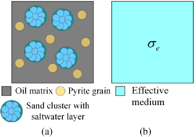
Figure 1: Three-phase GEMTIP model: (a) subsea reservoir multiphase heterogeneous model and (b) corresponding effective-medium model.

B. Construction of governing equations containing GEMTIP model

Based on the introduced GEMTIP complex conductivity model, the electromagnetic field governing equation of frequency domain CSEM method is constructed. Assuming the time harmonic factor e${}^{\mathrm{-}i}$${}^{\omega }$${}^t$ and ignoring the displacement current, in the case of quasi-static, Maxwell’s equations in the frequency domain containing the complex conductivity model can eliminate the magnetic field H in the formula after corresponding mathematical operations, and obtain the equation about the electric field E:

$$\nabla \times \nabla \times \mathbf{E}+i\omega {\mu }_0{\sigma }_e\mathbf{E}=-i\omega {\mu }_0{\mathbf{J}}_{\mathbf{s}},$$

(5)

where E is the electric field, ${\mathbf{J}}_{\mathbf{s}}$ is the electric source-current density, $\omega$ is the angular frequency, $\mu$${}_0$is the permeability in a vacuum and $\sigma$${}_e$ is the complex conductivity of the GEMTIP model. The above equation contains only one unknown electric field E, which can be solved directly. After the solution is completed, the electric field E can be substituted into the expression of Faraday’s electromagnetic induction law to obtain the magnetic field H, thus reducing the overall calculation amount.

C. Grid generation and application of emission source

In order to overcome the influence of electromagnetic field source singularity on numerical results and make the electromagnetic field component approximate to zero when propagating to the Dirichlet boundary, we use a non-uniform grid to divide the submarine reservoir model [29]. We first use the seafloor surface as the interface and divide the grid of the model into two parts, where the upper grid consists of the seawater layer and the lower grid consists of the sediment layer. Then we place the transmitter and receiver on the seabed to simulate the process of electromagnetic excitation and response measurement. Finally, we use a fine grid to divide the central region of the emission source, and a variable step length coarse grid to divide other regions to obtain a large enough calculation area. The mesh size increases from the center to the outside, thereby improving the calculation efficiency and accuracy to a certain extent. The mesh division form of the three-dimensional finite-difference frequency-domain (FDFD) is shown in Fig. 2. The spatial positions of the electric and magnetic components are set on the grid, with the electric components located in the center of the edge of the hexahedron and the direction parallel to the tangent vector of the corresponding edge, and the magnetic components located in the center of the face of the hexahedron and the direction parallel to the normal vector of the corresponding plane [30]. Each electric field component is surrounded by four magnetic fields, each magnetic field component is surrounded by four electric fields, and the electromagnetic field component is staggered sampled and diffused to the surrounding area.

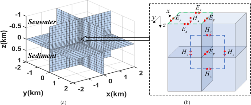
Figure 2: Mesh settings of 3D FDFD: (a) non-uniform grid containing seawater and sediment layers and (b) spatial distribution of electromagnetic field components.

In terms of the selection of emission source, this author selects the electrical source commonly used in marine CSEM exploration as the emission source. The loading method of the electrical source is shown in Fig. 3. Tx is the emission source, whose loading position is the same as the spatial sampling position of the electric field component, and the direction of the emission current is the same as the direction of the electric field on the edge. Rx is a receiver, arranged along the axis of the electrical source, which can be used to record electromagnetic signals. J${}_{s\mathit{}x}$ is the x direction component of current density ${\mathbf{J}}_{\mathbf{s}}$, and both J${}_{s\mathit{}y}$ and J${}_{s\mathit{}z}$components are set to zero. During the loading process of the emission source, a current needs to be applied. Assuming the current intensity is 1 A, the current density J${}_{s\mathit{}x}$ $=$ 1/$\mathrm{\Delta }$y$\mathrm{\Delta }$z, where $\mathrm{\Delta }$y and $\mathrm{\Delta }$z are the cell mesh sizes in the y and z directions.

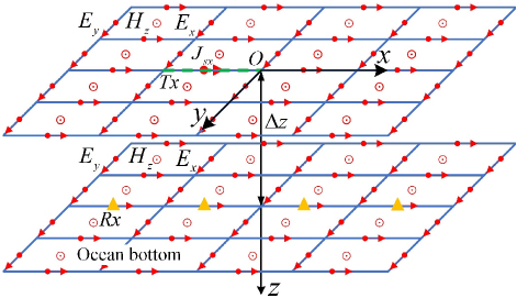
Figure 3: Spatial position of the electrical source.

D. Solution of FDFD linear equations

According to the spatial distribution of electromagnetic field components and the results of emission source loading, this paper uses the first-order central difference method to discrete the frequency domain electromagnetic field component expression containing the GEMTIP model in the Cartesian coordinate system. In order to facilitate further derivation and calculation, the difference equations are converted into matrix form by using the difference operator matrix, refer to equation (5), replace the magnetic field component in the expression, and get an equation containing only electric field component [31]:

$$\begin{array}{c}{\mathit{\text{J}}}_{sx}=-\left[\frac{{\delta }_{hzdy}{\delta }_{exdy}}{(-i\omega {\mu }_0)}+\frac{{\delta }_{hydz}{\delta }_{exdz}}{(-i\omega {\mu }_0)}+{\sigma }_e\right]{\mathit{\text{E}}}_x+\hfill \\ \left[\frac{{\delta }_{hzdy}{\delta }_{eydx}}{(-i\omega {\mu }_0)}\right]{\mathit{\text{E}}}_y+\left[\frac{{\delta }_{hydz}{\delta }_{ezdx}}{(-i\omega {\mu }_0)}\right]{\mathit{\text{E}}}_z\hfill \end{array},$$

(6)

	$\begin{array}{c}{\mathit{\text{J}}}_{sy}=\left[{\displaystyle \frac{{\delta }_{hzdx}{\delta }_{exdy}}{(-i\omega {\mu }_0)}}\right]{\mathit{\text{E}}}_x-\left[{\displaystyle \frac{{\delta }_{hxdz}{\delta }_{eydz}}{(-i\omega {\mu }_0)}}+{\displaystyle \frac{{\delta }_{hzdx}{\delta }_{eydx}}{(-i\omega {\mu }_0)}}+{\sigma }_e\right]\hfill \\ {\mathit{\text{E}}}_y+\left[{\displaystyle \frac{{\delta }_{hxdz}{\delta }_{ezdy}}{(-i\omega {\mu }_0)}}\right]{\mathit{\text{E}}}_z\hfill \end{array},$		(7)
	$\begin{array}{c}{\mathit{\text{J}}}_{sz}=\left[{\displaystyle \frac{{\delta }_{hydx}{\delta }_{exdz}}{(-i\omega {\mu }_0)}}\right]{\mathit{\text{E}}}_x+\left[{\displaystyle \frac{{\delta }_{hxdy}{\delta }_{eydz}}{(-i\omega {\mu }_0)}}\right]{\mathit{\text{E}}}_y-\hfill \\ \left[{\displaystyle \frac{{\delta }_{hydx}{\delta }_{ezdx}}{(-i\omega {\mu }_0)}}+{\displaystyle \frac{{\delta }_{hxdy}{\delta }_{ezdy}}{(-i\omega {\mu }_0)}}+{\sigma }_e\right]{\mathit{\text{E}}}_z\hfill \end{array},$		(8)

where E${}_x$, E${}_y$, E${}_z$, H${}_x$, H${}_y$ and H${}_z$are the column vectors of the electric field and the magnetic field respectively, $\delta$${}_{ezdy}$, $\delta$${}_{eydz}$, $\delta$${}_{exdz}$, $\delta$${}_{ezdx}$, $\delta$${}_{eydx}$ and $\delta$${}_{exdy}$ are the electric field difference operator matrices, representing the difference coefficients of the electric field in the x, y, z directions, and $\delta$${}_{hzdy}$, $\delta$${}_{hydz}$, $\delta$${}_{hxdz}$, $\delta$${}_{hzdx}$, $\delta$${}_{hydx}$ and $\delta$${}_{hxdy}$are the magnetic field difference operator matrices, representing the difference coefficients of the magnetic field in the x, y, z directions, respectively. The difference operator matrix is a large sparse matrix, which differentiates adjacent electromagnetic field components by non-zero elements 1 and $-$1. $\sigma$${}_e$ is a diagonal matrix, and the diagonal element represents the medium conductivity of each edge, which is equal to the volume average of the medium conductivity of the four adjacent grids.

In order to directly solve the linear equations containing the GEMTIP model, the above governing equations are transformed into the form MX $\mathrm{=}$ N, and the matrix of each component can be written as:

$$\mathit{\text{M}}=\left(\begin{array}{ccc}\hfill {\mathit{\text{M}}}_{11}\hfill & \hfill \frac{{\delta }_{hzdy}{\delta }_{eydx}}{(-i\omega {\mu }_0)}\hfill & \hfill \frac{{\delta }_{hydz}{\delta }_{ezdx}}{(-i\omega {\mu }_0)}\hfill \\ \hfill \frac{{\delta }_{hzdx}{\delta }_{exdy}}{(-i\omega {\mu }_0)}\hfill & \hfill {\mathit{\text{M}}}_{22}\hfill & \hfill \frac{{\delta }_{hxdz}{\delta }_{ezdy}}{(-i\omega {\mu }_0)}\hfill \\ \hfill \frac{{\delta }_{hydx}{\delta }_{exdz}}{(-i\omega {\mu }_0)}\hfill & \hfill \frac{{\delta }_{hxdy}{\delta }_{eydz}}{(-i\omega {\mu }_0)}\hfill & \hfill {\mathit{\text{M}}}_{33}\hfill \end{array}\right),$$

$$\mathit{\text{X}}=\left(\begin{array}{c}\hfill {\mathit{\text{E}}}_x\hfill \\ \hfill {\mathit{\text{E}}}_y\hfill \\ \hfill {\mathit{\text{E}}}_z\hfill \end{array}\right),\mathit{\text{N}}=\left(\begin{array}{c}\hfill {\mathit{\text{J}}}_{sx}\hfill \\ \hfill {\mathit{\text{J}}}_{sy}\hfill \\ \hfill {\mathit{\text{J}}}_{sz}\hfill \end{array}\right),$$

(9)

where M${}_{\mathrm{11}}$, M${}_{\mathrm{22}}$, and M${}_{\mathrm{33}}$are, respectively:

	$\begin{array}{c}{\mathit{\text{M}}}_{11}=-{\displaystyle \frac{{\delta }_{hzdy}{\delta }_{exdy}}{(-i\omega {\mu }_0)}}-{\displaystyle \frac{{\delta }_{hydz}{\delta }_{exdz}}{(-i\omega {\mu }_0)}}-{\sigma }_0\{1+{\displaystyle \sum _{l=1}^N}\hfill \\ \left[f_l{m}_l[1-{\displaystyle \frac{1}{1+{\left(i\omega {\tau }_l\right)}^{C_l}}}]\right]\}\hfill \end{array}.$		(10)
	$\begin{array}{c}{\mathit{\text{M}}}_{22}=-{\displaystyle \frac{{\delta }_{hxdz}{\delta }_{eydz}}{(-i\omega {\mu }_0)}}-{\displaystyle \frac{{\delta }_{hzdx}{\delta }_{eydx}}{(-i\omega {\mu }_0)}}-{\sigma }_0\{1+{\displaystyle \sum _{l=1}^N}\hfill \\ \left[f_l{m}_l[1-{\displaystyle \frac{1}{1+{\left(i\omega {\tau }_l\right)}^{C_l}}}]\right]\}\hfill \end{array}.$		(11)
	$\begin{array}{c}{\mathit{\text{M}}}_{33}=-{\displaystyle \frac{{\delta }_{hydx}{\delta }_{ezdx}}{(-i\omega {\mu }_0)}}-{\displaystyle \frac{{\delta }_{hxdy}{\delta }_{ezdy}}{(-i\omega {\mu }_0)}}-{\sigma }_0\{1+{\displaystyle \sum _{l=1}^N}\hfill \\ \left[f_l{m}_l[1-{\displaystyle \frac{1}{1+{\left(i\omega {\tau }_l\right)}^{C_l}}}]\right]\}\hfill \end{array}.$		(12)

Since most of the elements in the difference operator matrix are zero, in order to improve computing efficiency and reduce memory consumption, this paper stores the difference operator matrix of electric field and magnetic field as a large sparse matrix, and directly solves the matrix equation MX $\mathrm{=}$ N based on the built-in solver of MATLAB to calculate the column vectors of the electric field E${}_x$, E${}_y$, E${}_z$. Then, the calculated results are put into the magnetic field component expressions, and the magnetic field H${}_x$, H${}_y$, H${}_z$ can be obtained.

III. ALGORITHM CORRECTNESS VERIFICATION

In order to verify the correctness and effectiveness of the above 3D modeling method, the marine CSEM response in the frequency domain of a typical 1D reservoir model is calculated and compared with the semi-analytical solution. As shown in Fig. 4, the emission source is an electrical source, 50 meters away from the seabed surface, and is towed forward by the exploration vessel. The emission current is 1 A, the emission frequency is 1 Hz. The receivers are arranged on the seabed and maintain the same z coordinates. Assume that the first layer is seawater layer, the thickness is 1 km, and the conductivity is 3.2 S/m. The second layer is the seabed sediment layer, the thickness is 1 km, the conductivity is 1 S/m. The third layer is the oil layer containing IP, the thickness is 0.2 km, the measured or empirical values of GEMTIP model parameters and inclusion grains are shown in Table 1 [32]. The conductivity of oil matrix is 0.005, and the parameters of sand cluster with saltwater layer and pyrite are indicated by subscripts 1 and 2, respectively. The size of the target area is 20 km$\times$20 km$\times$11 km and its coordinate range is ($-$10 km, 10 km) $\times$ ($-$10 km, 10 km) $\times$ ($-$1 km, 10 km). The size of the Dirichlet extension boundary is 40 km$\times$40 km$\times$22 km and its coordinate range is ($-$20 km, 20 km)$\times$($-$20 km, 20 km)$\times$($-$1 km, 21 km), which is also the entire numerical simulation area. The number of discrete grid cells is 76$\times$76$\times$39. The fine grid size of emission source and IP layer region is 100 m$\times$100 m$\times$50 m and 200 m$\times$200 m$\times$100 m, respectively. Other areas are divided by coarse grid. The grid terminates at the boundary where Dirichlet boundary conditions have been applied.

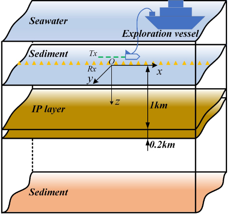
Figure 4: Schematic diagram of 1D reservoir model.

Table 1: GEMTIP conductivity-relaxation model for subsea reservoirs

Variable of Sand Cluster	Unit	Value	Variable of Pyrite	Unit	Value
$\sigma$${}_1$	S/m	1	$\sigma$${}_2$	S/m	15
f${}_{\mathrm{1}}$	%	6	f${}_{\mathrm{2}}$	%	3
C${}_{\mathrm{1}}$	—	0.8	C${}_{\mathrm{2}}$	—	0.6
a${}_{\mathrm{1}}$	mm	0.5	a${}_{\mathrm{2}}$	mm	0.2
$\alpha$${}_1$	m${}^2$ / (S$\cdot$sec${}^{c_l}$)	0.5	$\alpha$${}_2$	m${}^2$ / (S$\cdot$sec${}^{c_l}$)	2

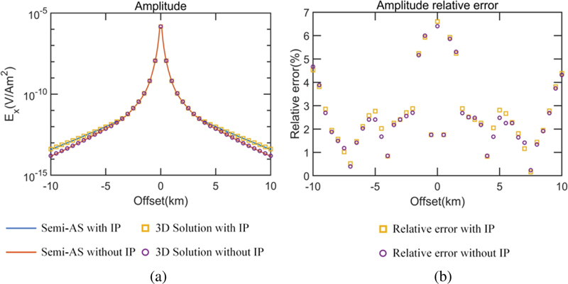
Figure 5: Comparison of electromagnetic response and semi-analytical solution (semi-AS) of 1D reservoir model: (a) amplitude curve and (b) relative error curve.

The 1D semi-analytical solution and the results of the forward modeling algorithm proposed in this paper are shown in Fig. 5. The solid blue line represents the 1D semi-analytical solution with IP, and the square represents the 3D numerical solution of the layered model with IP. The solid red line represents the 1D semi-analytical solution without IP, and the circle represents the 3D numerical solution of the layered model without IP. As can be seen from Fig. 5, the electromagnetic response curves of the 3D simulation solution of the reservoir model with or without IP are basically consistent with those of the semi-analytical solution. The electromagnetic response E${}_x$ (unit: V/Am${}^2$) in Fig. 5 is the normalized value of the electromagnetic signal acquired by the receiver to the electric dipole moment of the emission source, where the electric dipole moment is determined by the product of the emission current and the antenna length, i.e., V/m divided by Am [33]. The offset in Fig. 5 is the relative horizontal distance between the emission source Tx and the receiver Rx, which is measured in km. When the offset is between 2 km and 9 km, the amplitude relative error is less than 2.9% and 2.8%, respectively, indicating that the frequency-domain finite-difference algorithm based on the GEMTIP model has relatively high precision.

IV. ANALYSIS OF INDUCTION-POLARIZATION RESPONSE CHARACTERISTICS

A. 3D reservoir model

According to the research and discussion of reservoir IP mechanism in recent years, the IP effect will occur both in the reservoir itself and in the formation above it. In order to simulate the above rock and ore geological conditions, we first establish a 3D reservoir model. The settings of the transmitter and receiver are consistent with those in Fig. 4, the vacuum permeability $\mu$${}_0$is 4$\pi$$\times$10${}^{-7}$H/m, and the conductivity of the seabed sediments is 1 S/m. The location of the IP abnormal body is shown in Fig. 6, and its vertical distance from the z axis is 1 km. Tables 2 and 3 list IP parameters and geometry parameters of the reservoir model respectively. The variables t, d and s in Table 3 are the thickness, buried depth and geometrical size of the IP body. The size of the target area and the Dirichlet extension boundary are consistent with those in 1D reservoir model. The number of discrete grid cells is 68$\times$68$\times$49. The fine grid size of emission source and IP body region is also 100 m$\times$100 m$\times$50 m and 200 m$\times$200 m$\times$100 m, respectively. Other areas are divided by a coarse grid. Then, 3D numerical simulation of the reservoir models with different IP parameters and geometry parameters is carried out to analyze the marine CSEM induction-polarization response characteristics.

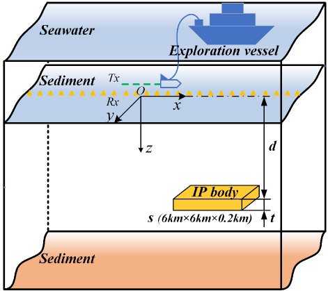
Figure 6: 3D reservoir model.

Table 2: IP parameters of 3D reservoir model

Variable	Unit	GEMTIPModel a	GEMTIPModel b	GEMTIPModel c	GEMTIPModel d
$\sigma$${}_0$	S/m	0.001;0.002;0.005;0.01	0.005	0.005	0.005
$\sigma$${}_1$	S/m	1	1	1	1
$\sigma$${}_2$	S/m	15	15	15	15
f${}_{\mathrm{1}}$	%	5	2;5;7;9	5	5
f${}_{\mathrm{2}}$	%	3	3	3	3
C${}_{\mathrm{1}}$	—	0.8	0.8	0.2;0.5;0.8;1	0.8
C${}_{\mathrm{2}}$	—	0.6	0.6	0.6	0.6
a${}_{\mathrm{1}}$	mm	2	2	2	0.5;1;2;5
a${}_{\mathrm{2}}$	mm	0.2	0.2	0.2	0.2
$\alpha$${}_1$	m${}^2$ / (S$\cdot$sec${}^{c_l}$)	0.5	0.5	0.5	0.5
$\alpha$${}_2$	m${}^2$ / (S$\cdot$sec${}^{c_l}$)	2	2	2	2

Table 3: Geometry parameters of 3D reservoir model

Variable	Unit	Model 1	Model 2	Model 3
t	m	100;200;300;400	200	200
d	m	1000	1000;1100;1200;1300	1000
s	—	6 km$\times$6 km$\times$0.2 km	6 km$\times$6 km$\times$0.2 km	4 km$\times$4 km$\times$0.2 km; 5 km$\times$5 km$\times$0.2 km; 6 km$\times$6 km $\times$0.2 km; 7 km$\times$7 km$\times$0.2 km

In order to analyze the influence characteristics of IP parameters of reservoir model on the marine CSEM induction-polarization response, we set the matrix conductivity $\sigma$${}_0$ as 0.001, 0.002, 0.005, and 0.01, the volume fraction f${}_{\mathrm{1}}$ as 0.02, 0.05, 0.07, and 0.09, the relaxation parameters C${}_{\mathrm{1}}$ as 0.2, 0.5, 0.8, and 1, and the grain radius a${}_{\mathrm{1}}$as 0.5, 1, 2, and 5, respectively, according to the four models in Table 2, while keeping other parameters unchanged.

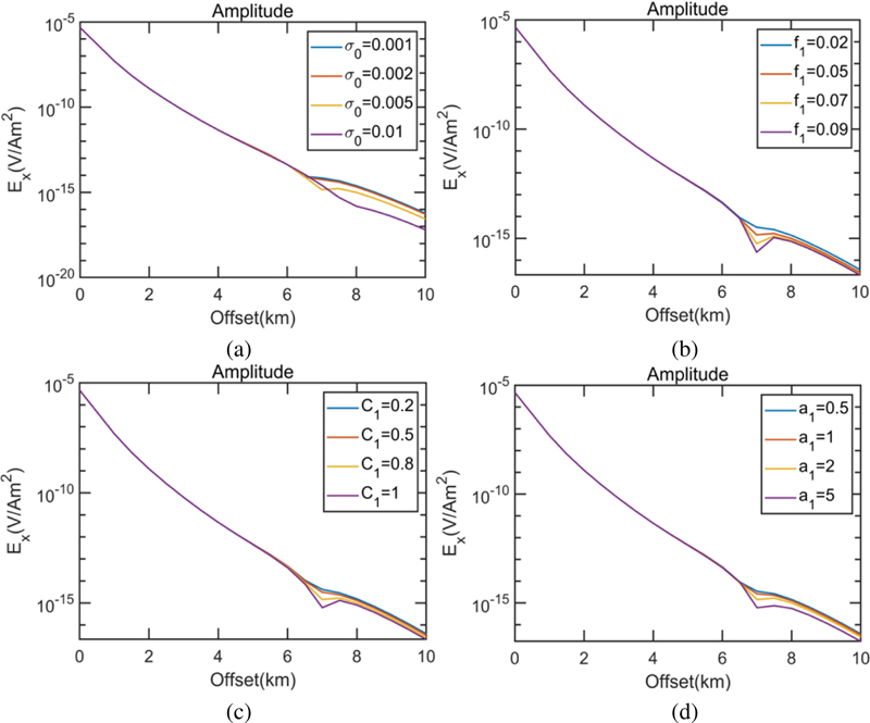
Figure 7: Induction-polarization response curves of different IP parameters under reservoir polarization mode: (a) response curves of different matrix conductivity, (b) response curves of different volume fraction, (c) response curves of different relaxation parameter and (d) response curves of different grain radius.

Figure 7 shows the marine CSEM induction-polarization response curves under different matrix conductivity, volume fraction, relaxation parameter and grain radius. It can be seen from Fig. 7 (a) that, with the increase of matrix conductivity $\sigma$${}_0$, the variation amplitude of induction-polarization response gradually increases. As can be seen from Fig. 7 (b), when other parameters remain unchanged, the variation amplitude of induction-polarization response first increases and then decreases as the volume fraction f${}_{\mathrm{1}}$ increases. It can be seen from Fig. 7 (c) that the larger the relaxation parameter C${}_{\mathrm{1}}$is, the variation amplitude of the induction-polarization response firstly increases and then decreases until it gradually becomes stable. As can be seen from Fig. 7 (d), when other parameters are unchanged, with the increase of grain radius a${}_{\mathrm{1}}$, the variation amplitude of induction-polarization response increases first and then decreases. As can be seen from Fig. 7, matrix conductivity has the greatest influence on the induction-polarization response results, followed by the volume fraction. Relaxation parameters and grain radius have relatively little influence.

In order to analyze the influence law of geometry parameters of reservoir model on the marine CSEM induction-polarization response, the thickness t is set as 100, 200, 300, and 400, the buried depth d is set as 1000, 1100, 1200, and 1300, the size s is set as 4 km$\times$4 km$\times$0.2 km, 5 km$\times$5 km$\times$0.2 km, 6 km$\times$6 km$\times$0.2 km and 7 km$\times$7 km$\times$0.2 km, and then forward modeling is carried out. The specific parameters are shown in Table 3. In the IP parameters, the matrix conductivity $\sigma$${}_0$is 0.005, the volume fraction f${}_{\mathrm{1}}$ is 0.05, the relaxation parameter C${}_{\mathrm{1}}$is 0.8, the grain radius a${}_{\mathrm{1}}$is 2, and the other parameters remain unchanged.

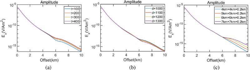
Figure 8: Induction-polarization response curves of different geometry parameters under reservoir polarization mode: (a) response curves of different polarized layer thickness, (b) response curves of different polarized layer buried depth and (c) response curves of different polarized layer size.

Figure 8 shows the marine CSEM induction-polarization response curves under different polarized layer thickness, buried depth and size. As can be seen from Fig. 8 (a), with the increase of the thickness t of the polarized layer, the amplitude of the induction-polarization response gradually increases, and the variation amplitude increases first and then becomes stable. As can be seen from Fig. 8 (b), when IP parameters, thickness and size of the polarized layer remain unchanged, the amplitude of the induction-polarization response gradually decreases with the increase of the buried depth d of the polarized layer. The variation amplitude first increases and then decreases. As can be seen from Fig. 8 (c), when IP parameters, thickness and buried depth of the polarized layer remain unchanged, the amplitude of the induction-polarization response gradually increases with the increase of the size s of the polarized layer. The variation amplitude gradually increases until it becomes stable. It can be seen from Fig. 8 that the size of the polarized layer has the greatest influence on the marine CSEM induction-polarization response, followed by the thickness of the polarized layer. The influence of the buried depth of the polarized layer is relatively weak.

B. 3D secondary pyrite model

According to the above analysis, this section will design a 3D secondary pyrite model, which is composed of three-phase medium: matrix sedimentary rock, carbonates with saltwater layer and pyrite [34, 35], in which carbonates with saltwater layer and pyrite are “conductive grains” and sedimentary rocks are “matrix bodies”. The settings of the transmitter and receiver are consistent with those in Fig. 6. Vacuum permeability $\mu$${}_0$and submarine sediment conductivity are the same as above. The conductivity of the reservoir is 0.01 S/m and the size is 6 km$\times$6 km$\times$0.2 km. The IP abnormal body position in the pyrite polarization mode is shown in Fig. 9, and its vertical distance from the z axis is 1 km. Tables 4 and 5 list IP parameters and geometry parameters of the secondary pyrite model, respectively. The conductivity $\sigma$${}_0$of the matrix sedimentary rocks is 0.005, and the parameters of carbonates with saltwater layer and pyrite are indicated by subscript 1 and 2, respectively. The size of the target area, the Dirichlet extension boundary, the number of discrete grids, the fine grid size of emission source and IP layer region are consistent with those in 3D reservoir model. Subsequently, we carry out 3D forward modeling of polarization models with different IP parameters and geometry parameters, then analyze the influence law of the above parameters on the marine CSEM induction-polarization response.

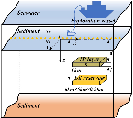
Figure 9: 3D secondary pyrite model.

Table 4: IP parameters of the 3D secondary pyrite model

Variable	Unit	GEMTIPModel e	GEMTIPModel f	GEMTIPModel g	GEMTIPModel h
$\sigma$${}_0$	S/m	0.001;0.002;0.005;0.01	0.005	0.005	0.005
$\sigma$${}_1$	S/m	0.5	0.5	0.5	0.5
$\sigma$${}_2$	S/m	15	15	15	15
f${}_{\mathrm{1}}$	%	5	5	5	5
f${}_{\mathrm{2}}$	%	8	4;8;12;16	8	8
C${}_{\mathrm{1}}$	—	0.6	0.6	0.6	0.6
C${}_{\mathrm{2}}$	—	0.8	0.8	0.2;0.5;0.7;1	0.8
a${}_{\mathrm{1}}$	mm	0.2	0.2	0.2	0.2
a${}_{\mathrm{2}}$	mm	2	2	2	0.2;0.5;1;2
$\alpha$${}_1$	m${}^2$ / (S$\cdot$sec${}^{c_l}$)	0.4	0.4	0.4	0.4
$\alpha$${}_2$	m${}^2$ / (S$\cdot$sec${}^{c_l}$)	2	2	2	2

Table 5: Geometry parameters of the 3D secondary pyrite model

Variable	Unit	Model 4	Model 5	Model 6
t	m	100;200;300;400	200	200
d	m	300	100;200;300;400	300
s	—	6 km$\times$6 km$\times$0.2 km	6 km$\times$6 km$\times$0.2 km	4 km$\times$4 km$\times$0.2 km; 5 km$\times$5 km$\times$0.2 km; 6 km$\times$6 km$\times$0.2 km; 7 km$\times$7 km$\times$0.2 km

In order to analyze the influence characteristics and rules of IP parameters of secondary pyrite model on the marine CSEM induction-polarization response, we set the matrix conductivity $\sigma$${}_0$ as 0.001, 0.002, 0.005, and 0.01. The volume fraction f${}_{\mathrm{2}}$as 0.04, 0.08, 0.12, and 0.16, the relaxation parameter C${}_{\mathrm{2}}$as 0.2, 0.5, 0.7, and 1, and the grain radius a${}_{\mathrm{2}}$as 0.2, 0.5, 1, and 2, according to the four models in Table 4, while the other parameters are kept unchanged.

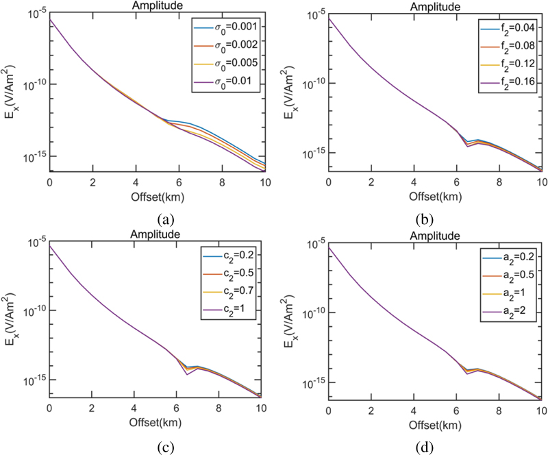
Figure 10: Induction-polarization response curves of different IP parameters under pyrite polarization mode: (a) response curves of different matrix conductivity, (b) response curves of different volume fraction, (c) response curves of different relaxation parameter and (d) response curves of different grain radius.

Figure 10 shows the marine CSEM induction-polarization response curves under different matrix conductivity, volume fraction, relaxation parameter and grain radius. As can be seen from Fig. 10 (a), with the increase of the matrix conductivity $\sigma$${}_0$, the amplitude of the induction-polarization response gradually decreases, and the variation amplitude gradually increases until it becomes stable. As can be seen from Fig. 10 (b), when other parameters remain unchanged, the variation amplitude of induction-polarization response first increases and then decreases as the volume fraction f${}_{\mathrm{2}}$increases. It can be seen from Fig. 10 (c) that the larger the relaxation parameter C${}_{\mathrm{2}}$is, the variation amplitude of the induction-polarization response shows a trend of first increasing and then decreasing until it gradually becomes stable. As can be seen from Fig. 10 (d), when other parameters remain unchanged, with the increase of grain radius a${}_{\mathrm{2}}$, the variation amplitude of induction-polarization response also first increases and then decreases. As can be seen from Fig. 10, matrix conductivity has the greatest influence on the induction-polarization response results, followed by the volume fraction. Relaxation parameter and grain radius have relatively little influence.

In order to analyze the influence of geometry parameters on the marine CSEM induction-polarization response, the thickness t of the polarized layer is set as 100, 200, 300, and 400, the buried depth d is set as 100, 200, 300, and 400. The size s is set as 4 km$\times$4 km$\times$0.2 km, 5 km$\times$5 km$\times$0.2 km, 6 km$\times$6 km$\times$0.2 km, 7 km$\times$7 km$\times$0.2 km, and then forward modeling is carried out. The specific parameters are shown in Table 5. In the IP parameter, the matrix conductivity $\sigma$${}_0$is 0.005, the volume fraction f${}_{\mathrm{2}}$is 0.08, the relaxation parameter C${}_{\mathrm{2}}$is 0.8, the grain radius a${}_{\mathrm{2}}$is 2, and the other parameters remain unchanged.

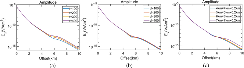
Figure 11: Induction-polarization response curves of different geometry parameters under pyrite polarization mode: (a) response curves of different polarized layer thickness, (b) response curves of different polarized layer buried depth and (c) response curves of different polarized layer size.

Figure 11 shows the marine CSEM induction-polarization response curves under different polarized layer thickness, buried depth and size. It can be seen from Fig. 11 (a) that, with the increase of the thickness t of the polarized layer, the amplitude of the induction-polarization response gradually increases and the variation amplitude first gradually increases and then becomes stable. As can be seen from Fig. 11 (b), when IP parameters, thickness and size of the polarized layer remain unchanged, the amplitude of the induction-polarization response gradually increases with the increase of the buried depth d of the polarized layer, and the variation amplitude first decreases and then increases. As can be seen from Fig. 11 (c), when IP parameters, polarized layer thickness and buried depth remain unchanged, the larger the polarized layer size s is, the amplitude of induction-polarization response gradually increases, and the variation amplitude gradually increases until it becomes stable. It can be seen from Fig. 11 that the size of the polarized layer has the greatest influence on the marine CSEM induction-polarization response results, followed by the thickness of the polarized layer. The influence of the buried depth of the polarized layer is relativelysmall.

V. CONCLUSION

In order to analyze the influence of physical properties and geometric characteristics of submarine reservoir and secondary pyrite on marine CSEM field, this paper introduces the GEMTIP model, adopts the FDFD method to calculate the induction-polarization response of reservoir and secondary pyrite model, and studies the influence characteristics of IP parameters and geometric parameters on the induction-polarization response under different polarization modes. Results show that the matrix conductivity of IP parameters in the reservoir self-polarization mode has the greatest influence on the induction-polarization response results, the volume fraction has the second influence, and the relaxation parameter and grain radius have relatively little influence. In addition, compared with the polarized layer thickness and buried depth, the polarized layer size of geometry parameters has more obvious influence on the induction-polarization response results. The effect of IP parameters and geometry parameters in the secondary pyrite polarization mode on the induction-polarization response is similar to that of the reservoir self-polarization mode. Therefore, the numerical calculation method of marine CSEM IP effect based on GEMTIP model proposed in this paper can provide a new tool for quantitative analysis of the influence of rock and ore structure, composition and fluid content on its conductive characteristics. The research is of great significance and value for understanding the relationship between submarine multiphase composite medium and electromagnetic wave propagation.

ACKNOWLEDGMENT

The authors would like to thank the reviewers and the editors for their valuable comments. This research was financially supported by the National Key Research and Development Program of China (Grant Number 2022YFC2807904).

REFERENCES

[1] K. A. Weitemeyer, S. Constable, and A. M. Tréhu, “A marine electromagnetic survey to detect gas hydrate at Hydrate Ridge, Oregon,” Geophys. J. Int., vol. 187, no. 1, pp. 45-62, June 2011.

[2] S. Constable, “Ten years of marine CSEM for hydrocarbon exploration,” Geophysics, vol. 75, no. 5, pp. 75A67-75A81, Oct. 2010.

[3] S. Constable, “Review paper: Instrumentation for marine magnetotelluric and controlled source electromagnetic sounding,” Geophys. Prospect., vol. 61, pp. 505-532, Jan. 2013.

[4] S. Hölz, A. Swidinsky, M. Sommer, M. Jegen, and J. Bialas, “The use of rotational invariants for the interpretation of marine CSEM data with a case study from the North Alex mud volcano, West Nile Delta,” Geophys. J. Int., vol. 201, no. 1, pp. 224-245, Jan. 2015.

[5] H. B. Chen, T. L. Li, H. Y. Shi, H. Wang, and S. P. Li, “An edge-based finite element method for 3D marine controlled-source electromagnetic forward modeling with a new type of second-order tetrahedral edge element,” Int. J. Appl. Electrom., vol. 57, no. 3, pp. 217-233, May 2018.

[6] M. W. Dunham, S. Ansari, and C. G. Farquharson, “Application of 3D marine controlled-source electromagnetic finite-element forward modeling to hydrocarbon exploration in the Flemish Pass Basin offshore Newfoundland, Canada,” Geophysics, vol. 83, no. 2, pp. WB33-WB49, Apr. 2018.

[7] J. H. Wang, B. Li, L. P. Chen, and Z. H. Wang, “Theoretical analysis and experimental measurements of electromagnetic radiation from a horizontal electric dipole in shallow sea,” Electromagnetics, vol. 37, no. 6, pp. 398-410, Apr. 2017.

[8] L. Slater and D. Glaser, “Controls on induced polarization in sandy unconsolidated sediments and application to aquifer characterization,” Geophysics, vol. 68, no. 5, pp. 1547-1558, Oct. 2003.

[9] C. Ulrich and L. Slater, “Induced polarization measurements on unsaturated, unconsolidated sands,” Geophysics, vol. 69, no. 3, pp. 762-771, June 2004.

[10] Z. X. He and X. B. Wang, “Oil/gas detection by electromagnetic survey,” Oil Geophys. Prospect., vol. 42, no. 1, pp. 102-106, Feb. 2007.

[11] P. C. Veeken, P. J. Legeydo, Y. A. Davidenko, E. O. Kudryavceva, S. A. Vanov, and A. Chuvaev, “Benefits of the induced polarization geoelectric method to hydrocarbon exploration,” Geophysics, vol. 74, no. 2, pp. B47-B59, Apr. 2009.

[12] D. Z. Wang, S. S. Yan, Z. J. Dong, X. D. Tan, Z. Li, and Y. H. Liu, “IP effect on marine CSEM based on two polarization modes of oil/gas reservoir,” Prog. Geophys. (in Chinese), vol. 30, no. 3, pp. 1304-1314, 2015.

[13] Y. W. Huang, “3D forward modeling and response analysis of the controlled source electromagnetic signal with IP effect,” M.S. thesis, School of Geophysics and Measurement-Control Technology, East China University of Technology, Nanchang, Jiangxi, China, June 2017.

[14] W. Q. Liu, P. R. Lin, Q. T. Lu, Y. Li, and J. H. Li, “Synthetic modelling and analysis of CSEM full-field apparent resistivity response combining EM induction and IP effect for 1D medium,” Explor. Geophys., vol. 49, no. 5, pp. 609-621, May2017.

[15] X. Z. Ding, Y. G. Li, and Y. Liu, “Influence of IP effects on marine controlled-source electromagnetic responses,” Oil Geophys. Prospect., vol. 53, no. 6, pp. 1341-1350, Dec. 2018.

[16] R. Mittet, “Electromagnetic modeling of induced polarization with the fictitious wave-domain method,” SEG Technical Program Expanded Abstracts, pp. 979-983, Aug. 2018.

[17] K. J. Xu and J. Sun, “Induced polarization in a 2.5D marine controlled source electromagnetic field based on the adaptive finite-element method,” Appl. Geophys., vol. 15, no. 2, pp. 332-341, June 2018.

[18] J. Li, Z. He, and N. Feng, “Induced polarization effects of 3D frequency domain MCSEM responses using finite volume method,” Int. J. Appl. Electrom., vol. 61, no. 4, pp. 491-507, May 2019.

[19] N. Qiu, Z. X. Luo, Q. C. Fu, Z. Sun, Y. J. Chang, and B. R. Du, “Identification of induced polarization of submarine hydrocarbons in marine controllable source electromagnetic exploration,” Front. Earth. Sc-Switz., vol. 10, pp. 1-24, Jan.2023.

[20] M. S. Zhdanov, “Generalized effective-medium theory of induced polarization,” Geophysics, vol. 73, no. 5, pp. 197-211, Oct. 2008.

[21] L. Fu, “Induced polarization effect in time domain: Theory, modeling, and applications,” M.S. thesis, Department of Geology and Geophysics, The University of Utah, Salt Lake City, UT, USA, Dec. 2011.

[22] X. L. Tong, L. J. Yan, and K. Xiang, “Modifying the generalized effective-medium theory of induced polarization model in compacted rocks,” Geophysics, vol. 85, no. 4, pp. 245-255, Aug.2020.

[23] C. R. Phillips, “Experimental study of the induced polarization effect using Cole-Cole and GEMTIP models,” M.S. thesis, Department of Geology and Geophysics, The University of Utah, Salt Lake City, UT, USA, Dec. 2010.

[24] M. S. Zhdanov, V. Burtman, and A. F. Marsala, “Carbonate reservoir rocks show induced polarization effects, based on generalized effective medium theory,” in Extended Abstracts of 75th EAGE Conference & Exhibition, pp. 1-5, June 2013.

[25] Y. J. Chang, T. Tohniyaz, and H. Y. Wang, “Influence factors of frequency-dependent coefficient with GEMTIP model,” Oil Geophys. Prospect., vol. 53, no. 5, pp. 1103-1109, Oct. 2018.

[26] V. Burtman, H. Y. Fu, and M. S. Zhdanov, “Experimental study of induced polarization effect in unconventional reservoir rocks,” Geomaterials, vol. 4, no. 4, pp. 117-128, Oct. 2014.

[27] M. S. Zhdanov, V. Burtman, M. Endo, and W. Lin, “Complex resistivity of mineral rocks in the context of the generalised effective-medium theory of the induced polarisation effect,” Geophys. Prospect., vol. 66, no. 4, pp. 798-817, May 2018.

[28] V. Burtman and M. S. Zhdanov, “Induced polarization effect in reservoir rocks and its modeling based on generalized effective-medium theory,” Resource-Efficient Tech., vol. 1, no. 1, pp. 34-48, July 2015.

[29] H. Klingbeil, K. Beilenhoff, and H. L. Hartnagel, “FDFD full-wave analysis and modeling of dielectric and metallic losses of CPW short circuits,” IEEE T. Microw. Theory, vol. 44, no. 3, pp. 485-487, Mar. 1996.

[30] Y. Kane, “Numerical solution of initial boundary value problems involving maxwell’s equations in isotropic media,” IEEE Trans. Antennas Propag., vol. 14, no. 3, pp. 302-307, May 1966.

[31] Y. J. Ji, H. S. Liu, Y. B. Yu, and X. J. Zhao, “3-D modelling and analysis of superparamagnetic effects in ATEM based on the FDFD,” Geophys. J. Int., vol. 231, no. 2, pp. 1252-1267, June 2022.

[32] V. Burtman, A. V. Gribenko, and M. S. Zhdanov, “Advances in experimental research of induced polarization effect in reservoir rocks,” SEG Technical Program Expanded Abstracts, pp. 2475-2479, Oct. 2010.

[33] S. Constable and L. J. Srnka, “An introduction to marine controlled-source electromagnetic methods for hydrocarbon exploration,” Geophysics, vol. 72, no. 2, pp. WA3-WA12, Apr. 2007.

[34] S. Z. Zhang, Y. X. Li, J. P. Zhou, X. W. Nie, A. C. Zhou, and G. D. Yang, “Induced polarization (IP) method in oil exploration – the cause of IP anomaly and it’s relation to the oil reservoir,” Chinese J. Geophys., vol. 29, no. 6, pp. 597-614, Nov. 1986.

[35] B. K. Sternberg, “A review of some experience with the induced polarization/resistivity method for hydrocarbon surveys: Successes and limitations,” Geophysics, vol. 56, no. 10, pp. 1522-1532, Oct. 1991.

BIOGRAPHIES

Chunying Gu (Graduate Student Member, IEEE) received the M.S. degree from the College of Mechanical and Vehicle Engineering, Hunan University, Changsha, China, in 2011. She is currently pursuing the Ph.D. degree in detection technology and automation from Jilin University, Changchun, China. Her research interests include 3D marine controlled-source electromagnetic (CSEM) modeling and data processing.

Suyi Li (Member, IEEE) received her M.Sc. and Ph.D. degrees both from Jilin University in 2002 and 2009, respectively. From 2008 to 2009, she studied at the University of Illinois at Urbana-Champaign as a joint Ph.D. Now she is a professor in Jilin University. Her main research interests include computer applications and digital signal processing.

Silun Peng received the Ph.D. degree from the College of Automotive Engineering, Jilin University, Changchun, China, in 2014. He is currently a deputy senior engineer with Jilin University. His research interests include, but are not limited to, computer applications, digital signal processing and hardware system design.

ACES JOURNAL, Vol. 39, No. 12, 1103–1115
doi: 10.13052/2024.ACES.J.391209
© 2024 River Publishers

ABSTRACT

I. INTRODUCTION

II. FDFD METHOD BASED ON GEMTIP MODEL

A. Introduction of the GEMTIP composite conductivity model

B. Construction of governing equations containing GEMTIP model

C. Grid generation and application of emission source

D. Solution of FDFD linear equations

III. ALGORITHM CORRECTNESS VERIFICATION

IV. ANALYSIS OF INDUCTION-POLARIZATION RESPONSE CHARACTERISTICS

A. 3D reservoir model

B. 3D secondary pyrite model

V. CONCLUSION

ACKNOWLEDGMENT

REFERENCES

BIOGRAPHIES