Fast FDTD/TDPO Hybrid Method Based on Spatiotemporal Sparse Sampling
Linxi Wang and Juan Chen
School of Information and Communications Engineering
Xi’an Jiaotong University, Xi’an 710049, People’s Republic of China
wanglinqian@stu.xjtu.edu.cn, chen.juan.0201@mail.xjtu.edu.cn
Submitted On: September 25, 2024; Accepted On: March 4, 2025
ABSTRACT
Based on a hybrid method of finite-difference time-domain (FDTD) and time-domain physical optics (TDPO), this study employs a sparse sampling technique in near-to-far-field calculations to improve the efficiency of electrical large target computation. In the conventional hybrid method, the transformation from the near-field of the FDTD region to the far-field of the TDPO region involves the largest amount of computation, which can be reduced by applying the sparse sampling optimization method jointly in spatial and time domain. Compared to the conventional method, our proposed algorithm significantly reduces computation time while maintaining a negligible increase in error. Several examples are provided to demonstrate the accuracy and efficiency of our approach. In particular, a large parabolic antenna whose aperture size is 100 wavelengths is computed. The computation time is decreased by up to 91.52% of the conventional method while the maximum relative error is -21.56 dB. Compared with results of CST software, the method proposed in this work has smaller errors and excellent applicability.
Index Terms: Far-field, finite-difference time-domain, hybrid method, parabolic antenna, sparse sampling, time-domain physical optics.
I. INTRODUCTION
Benefiting from the rapid development of computer technology and hardware, transient electromagnetic scattering simulations of composite objects with diverse sizes and material properties are widely applied in fields such as aerospace [1], radar [2] and marine [3]. In practical scenarios, the electromagnetic challenges that need to be addressed are often multiscale in nature [4, 5]. For instance, a large reflector antenna is much larger than a typical wavelength, while its feed structure is an electrical fine structure with respect to a typical wavelength. However, as the electrical scale of the target increases, the demands in computational time and resource requirements by numerical methods become overwhelming.
With the aim of computing the transient electromagnetic scattering accurately and efficiently, hybrid methods have been proposed by researchers to address challenges that cannot be remedied easily by a single method [6–9]. A hybrid schema combining finite-difference time-domain (FDTD) [10] and time-domain physical optics (TDPO) [11], as a representative computational method in time domain, demonstrates significant advantages in broadband calculations [12]. The FDTD method enables accurate simulations across various electromagnetic problems, while the TDPO can reduce memory requirements and enhance computational speed. Yang et al. [13] systematically investigated the hybrid algorithm of FDTD and TDPO, conducting far-field scattering calculations for composite targets comprising dipole and perfect electric conductor (PEC) plates. This method needs small amounts of computer memory and achieves high efficiency compared to a full wave solution. However, the examples in the literature are too simple to demonstrate the efficiency. The antenna models in practical engineering applications tend to be more complex and larger in scale. As discussed in [14], the radiation fields of the large single reflector calculated by a hybrid method parallelized-FDTD and parallelized-TDPO, which demonstrated the ability to simulate a large reflector with dimensions spanning hundreds of wavelengths, included cases where the reflector’s feed is offset. Indeed, conventional hybrid methods face significant limitations when addressing multiscale problems, primarily due to excessive computational demands. These challenges often render such methods either impractical or prohibitively slow, especially when the antenna aperture exceeds several hundred wavelengths or the feed structure becomes increasingly complex, frequently necessitating the use of parallel algorithms. Furthermore, there is currently a scarcity of literature offering a comparative analysis of computation time for such hybrid algorithms.
This paper presents an optimization of the conventional FDTD/TDPO hybrid algorithm by employing a sparse sampling technique in both spatial and time domains, which reduces computational workload and enhances efficiency. Our proposed approach achieves the computation of large parabolic antennas fed by various sources using a serial algorithm, a task previously limited to parallel algorithms as reported in [14]. Importantly, the computation time is significantly saved without a substantial increase in errors compared to conventional hybrid algorithms.
The rest of this paper is organized as follows. The principle of the hybrid method including the formulation of the coupling between the FDTD method and TDPO method and the implementation process of organization have been presented in detail in section II. Through providing several numerical examples, section III demonstrates the accuracy and efficiency of the proposed hybrid method for large composite targets transient electromagnetic scattering. Finally, conclusions are presented in section IV.
II. BASIC THEORY
When using the FDTD/TDPO hybrid method to study complex composite objects, the computation domain is first divided into sub-domains based on configuration: the FDTD region containing small-size objects with fine structures, and the TDPO region containing large electrical dimensions. Conducting far-field scattering calculations is divided into primary scattering and secondary scattering. The primary scattered field involves direct far-field scattering by the FDTD and TDPO regions, which can be calculated separately using FDTD and TDPO methods. The secondary scattered field is due to the mutual-coupling between the FDTD and TDPO region. The scattered field from one region is considered to be the incident field on the other region.
The key point of the hybrid algorithm lies in the coupling between the two regions, which is also crucial for optimization. Let us take the coupling from the FDTD region to the TDPO region as an example. Firstly, the magnetic fields on the FDTD extrapolation surface are calculated using the FDTD method. Then, the magnetic fields in the TDPO region are computed via near-to-far-field extrapolation. Finally, the far-fields of TDPO region are obtained using the TDPO method.
The near-to-far-field extrapolation technique is based on Kirchhoff’s surface integral representation (KSIR) [15]. A cubic surface S is selected as the extrapolation surface. The surface S should be closed, enclosing all sources, and as small as possible. Taking the magnetic field along the x-axis as an example, assuming a point P exists outside the surface S, the extrapolated magnetic field H from the FDTD extrapolation surface to the TDPO calculation domain surface element is:
| (1) |
where r is the position vector of the observation point P, r is the position vector of any point on the closed surface S, R r-r, R |R|, is the outward-pointing normal to the FDTD extrapolation surface, is the retarded time and c is the speed of light in free space.
At time step n+1, the partial derivatives with respect to space and time are represented by second-order center differences:
| (2) | ||
| (3) |
represents the value of H at time step n, t is time-step size, z is the grid size in the z-direction. Substituting equations (2) and (3) into equation (1) yields:
| (4) |
where:
| (5) | ||
| (6) | ||
| (7) | ||
| (8) | ||
| (9) |
Here, is the area of Yee’s cell on the xy plane at z kandR is the distance from each subsurface to the observation point.
To reduce memory usage and enhance computational speed, a sequential transfer method [13] is employed. In this method, for each time step computed by FDTD, the field values on the extrapolation surface of the Yee cell are extrapolated to the surface triangular patches of the TDPO region using KSIR. Then, the contribution from each patch to the far-field observation point can be immediately computed using the TDPO method. The far-field values are summed up based on the time delay between cell-to-patch and patch-to-observation point until the transient process is completed.
However, conventional hybrid algorithms face significant challenges when dealing with large antenna apertures and complex feed structures. Large-aperture antennas are often electrically large, requiring a dense grid to accurately model the electromagnetic behavior, which leads to a high grid count. The complexity of the feed structure further exacerbates this issue by demanding smaller and denser grids to capture the fine details, which results in an increased computational load. Moreover, the smaller time step required to maintain numerical stability in such cases can lead to a further increase in computation time. Moreover, the extrapolation step is the most time-consuming part of the entire calculation process. In each time step, it is necessary to calculate extrapolated field values from each Yee cell on the extrapolation surface of the FDTD region to each triangle on the TDPO region.
Here, we propose two optimization strategies: spatial sparse sampling to reduce grid count and temporal sparse sampling to enable larger time step. These two methods can be applied jointly to significantly enhance computational efficiency.
A. Spatial sparse sampling method
Considering the impact of fine structures on the accuracy, the grid size of the targets within the FDTD region is typically set to be small. Consequently, the number of grids on the extrapolation surfaces becomes very large, resulting in a significant computational burden and extremely long computation times during near-field extrapolation. In general, the number of grids on the extrapolation surfaces Kis in the order of 10 to 10, while the order of magnitude of cells in the TDPO region M is 10 to 10. Thus, the total extrapolation time will be KM, reaching up to 10 times that of one single extrapolation. Consequently, extrapolation becomes a significant bottleneck in overall computation, particularly when addressing electromagnetic problems with electrically small and intricate structures. As an example, consider a composite target whereK is 10000 and M is 1000. By applying sparse sampling to K, where every two grid points are sampled once, K can be reduced to 5000. This decreases the total number of extrapolations from 10 to 510, thereby significantly reducing the computational cost.
When conducting near-field extrapolation, it is unnecessary to substitute the value of each cell into equation (1). The spatial sparse sampling method involves sampling on the extrapolation surface and then performing extrapolation. Due to the presence of fine structures in the feed, the grids on the extrapolation surface will be dense. However, these overly dense grids are required because the grid partitioning must fit the structure and shape of the target. Since the field variations in these areas are not drastic, selectively extracting grids at intervals on the extrapolation surface for extrapolation calculations does not affect the collection of field values on the extrapolation surface outside the FDTD region and thus does not significantly impact the final results. Therefore, the extrapolation operation with interval sampling will not affect the accuracy of the results significantly but can effectively reduce the computational load.
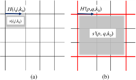
Figure 1: Grid setting (a) without spatial sampling and (b) with spatial sampling set to 3.
Taking the xy-plane as an example, Fig. 1 depicts a schematic diagram of the grid setting when the spatial sampling is set to 3. The black grid lines represent the original FDTD grid, while the red lines represent the sampling grid. Let (i,j,k) denote the magnetic field on the original grid, (p,q,k) denote the magnetic field on the sampling grid, s(i,j,k) denote the area of the original grid, s(p,q,k) denote the area of the sampling grid, M andN denotes the number of original grids in the x and y directions, and Ms andNs denotes the number of sampling grids in the x and y directions, respectively. Then, we have:
| (10) |
In equation (10), (p,q,k) can be approximated using the average value method. If the number of intervals in the spatial grid is G, then the magnetic field components on the sampling grid can be approximated by the average value method as follows:
| (11) |
By substituting equations (5), (6) and (7) into equation (4), the equation can be expressed as:
| (12) |
Substituting equation (11) into equation (12) gives:
| (13) |
Here, Ms INT((M-1)/G) and Ns INT((N-1)/G).
By comparing equations (12) and (13), the absolute error after sparsification of the spatial grid can be derived:
| (14) |
From equation (14), it can be seen that is mainly influenced by the difference and the product . Therefore, the error is likely to increase in two situations: first, where the field components vary sharply and, second, where the original FDTD grid is too coarse. Thus, in regions with significant field variation, such as at apertures, material boundaries and interfaces between different media, the grid discretization should be appropriately increased to mitigate the impact of spatial sparsity on the results.
B. Time sparse sampling method
In each time step of the current conventional algorithm, the near-field values are computed first by FDTD, then the magnetic field in the TDPO region is extrapolated using KSIR, and finally TDPO is used to calculate the far-field. The FDTD algorithm must comply with the Courant-Friedrichs-Lewy (CFL) condition [16] to guarantee the stability of the solution, which means that the time-step size of the FDTD algorithm is related to the minimum grid size in the three spatial directions. To reduce numerical dispersion caused by spatial discretization, the maximum grid size in the FDTD method is typically less than one-tenth of the shortest wavelength. When the object has fine structures, the minimum grid size may be only one-hundredth of the wavelength or even smaller. Therefore, the time step of the FDTD method is much smaller than that of the TDPO method. As the time step decreases, the number of time steps that need to be calculated increases, resulting in a greater computational load.
According to the time-domain sampling theorem, a band-limited signal f(t) with a maximum frequency f can be uniquely represented by uniformly distributed samples, provided the sampling interval does not exceed 1/2f. The time sparse sampling method optimizes FDTD by storing the field values on the extrapolation surface every N time steps. Subsequently, near-field extrapolation is performed using the Kirchhoff surface integral, and the far-field values for each time step are computed using the TDPO method. According to the Nyquist sampling theorem, the sampling interval only needs to satisfy (N-1)t1/(2f), which significantly reduces the number of iterations required for the extrapolation steps. Here t is the time-step length of FDTD and f denotes the maximum operating frequency.
III. NUMERICAL RESULTS
To illustrate the efficiency, accuracy and applicability of the proposed approach, we present two numerical cases. In the first case, a basic composite entity comprising both small-scale and large-scale structures relative to the wavelength is given and simulated. Various sets of sampling data are configured to assess the influence of the sampling number on result errors. A comparative analysis is conducted between the conventional FDTD/TDPO approach and the proposed FDTD/TDPO method, focusing on their efficiency and accuracy. In the second case, the applicability of the proposed approach to problems concerning a large parabolic antenna is demonstrated. Additionally, the findings are corroborated through validation using the commercial software CST.
A. Cube and plate
In the first example, we consider a PEC cube located at a distance of 10 in front of a PEC plate. The metallic cube has a side length of 1, while the plate measures 1001001. A modulated-Gaussian pulse plane wave with a frequency band 1020 GHz is incident along the z-axis, with the electric field polarized parallel to x-axis. The result of the hybrid method is compared with that of FDTD to confirm the accuracy of the hybrid method. Figure 2 shows the transient far-field scattering response calculated by the conventional FDTD/TDPO hybrid method and the FDTD method.
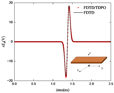
Figure 2: Far-field in time domain.
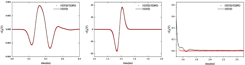
Figure 3: Far-field for the time interval of (a) 0-0.8 ns, (b) 1-2 ns and (c) 1.5-2.5 ns.
It is evident that the two results are in good agreement. Due to the significant difference of four orders of magnitude in the field values between the FDTD region and TDPO region, the results are segmented by time intervals. Figure 3 (a) depicts the far-field for the time interval of 0-0.8 ns, representing the primary scattering from the small PEC cube. Figure 3 (b) illustrates the far-field for the time interval of 1-2 ns, representing the sum of the primary scattering from the plate and the coupled field between the plate and the cube. Figure 3 (c) presents the far-field values after 1.5 ns.
Overall, the backscattering fields of the combined target computed by two methods match well, with discrepancies emerging only after 1.5 ns. Such discrepancies are mainly attributed to the TDPO method only considering the induced currents on the plate surface, without considering the edge diffraction fields.
In the two algorithms, the FDTD algorithm took 16.23 hours while the FDTD/TDPO hybrid algorithm required 144.49 hours, indicating the need for optimization of the hybrid algorithm in terms of computation time. Therefore, we use spatial sparse sampling and time sparse sampling methods for optimization, and focus on analyzing the error in the coupling part of theresults.
First, we fix the time sample at 5. Five sets of data with spatial sample of 1, 2, 4, 6 and 8 are selected for comparison over 500 time steps. Figure 4 shows the comparison of far-field obtained with different spatial samples, which are in good agreement. The relative errors of the far-field calculated with spatial sample of N 2, 4, 6 and 8 compared to the case of no sampling interval (i.e., N 1) are displayed in Fig. 5. The error is defined as a function of time by:
| (15) |
where represents the electric field with spatial sample of N (N1), and represents the electric field with spatial sample of 1.
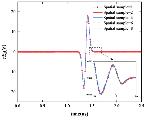
Figure 4: Comparison of far-fields by different spatial samples.
There are no relative error values in the earlier time segments because the algorithms for computing the primary scattering are the same, resulting in a relative error of 0. As can be seen in Fig. 4, the more sampling points there are, the smaller the error. However, excessive sampling leads to longer computation times, defeating the purpose of optimizing the algorithm.
Before 1.2 ns, there are no numerical errors in the earlier time segments because the algorithms for computing the primary scattering are the same, resulting in an infinitely small relative error. Taking a spatial sampling interval of 2 as an example, as shown in Fig. 3, a distinct time-domain waveform appears after 1.25 ns. Correspondingly, in Fig. 5, the relative error undergoes a rapid change between 1.25 ns and 1.4 ns, increasing to -128.05 dB, and then stabilizes between -172 dB and -113 dB. Figure 5 also shows that as the spatial sampling interval increases, the error slightly increases, though not significantly. Larger errors tend to occur when the electric field is near its peaks or troughs, leading to greater relative error. Conversely, when the electric field is near zero, the relative error is reduced. Therefore, the relative error fluctuates rather than remaining constant.
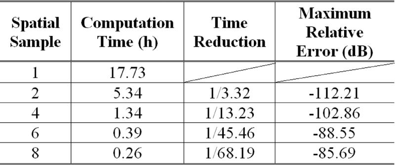
Table 1 presents the computation time and the maximum relative error corresponding to different spatial samples. As the spatial sample increases from 2 to 8, the maximum relative error increases from -112.21 dB to -85.69 dB, while the computation time decreases from 1064.03 min to 15.76 min. When the spatial sample is set to 10, the time is reduced to 1/67.51 of the original, indicating a substantial reduction in time. Although the increase in error with the larger spatial sample interval is not significant, the substantial reduction in time greatly enhances the computational capability of the hybrid algorithm.
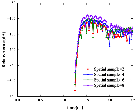
Figure 5: Relative error of different spatial samples.
Table 1: Computation time and maximum relative error of different spatial samples
Subsequently, we analyze the time sparse sampling. With spatial sample fixed at 4, five sets of data with time sample of 1, 2, 4, 8 and 16 are selected for comparison over 500 time steps. Figure 6 illustrates the far-field scattering results for different time samples, while Fig. 7 contrasts the relative errors corresponding to these time samples.
One can see that as the time sample increases, the sampling points become sparser, making it more likely to miss peaks or troughs in the field values, thus leading to larger errors. However, with the increase in the time sample, the maximum relative error fluctuates slightly, consistently remaining below -78 dB.
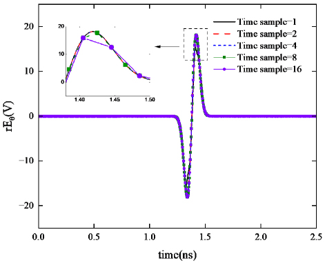
Figure 6: Comparison of far-fields by different time samples.
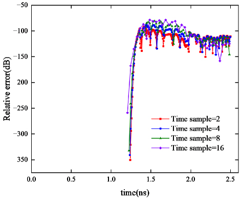
Figure 7: Relative error of different time samples.
Table 2: Computation time and maximum relative error of different time samples

The time required is reduced to 1/21.63 of that when the time sample is 1, as shown in Table 2. Consequently, although the increase in the time sample does not significantly increase the error, there is a significant reduction in time consumption, thereby notably enhancing the computational efficiency of the hybrid algorithm.
B. Parabolic antenna fed by horn
Here we consider an example of a composite target consisting of a parabolic antenna and a horn antenna, as depicted in Fig. 8.
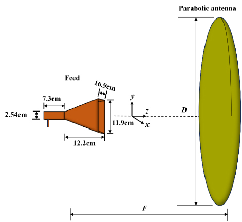
Figure 8: Parabolic antenna fed by horn.
The horn antenna is placed as the feed source at the focus of the parabolic antenna. The operating frequency is f 6 GHz, the aperture diameter of the parabolic antenna is D 100, and the focal-to-diameter ratio is F/D 0.685, where F denotes the focal length of the parabolic antenna. The waveguide length in the horn antenna is 7.3 cm, with a waveguide aperture size of 0.05080.0254 cm. The axial projection length of the horn is 12.2 cm and its aperture size is 16.911.9 cm. The horn antenna is excited by a coaxial feed with a Gaussian pulse signal.
The horn antenna in the FDTD computation domain is discretized using non-uniform hexahedral grids, comprising 713175 cells. The minimum grid sizes in the three directions are 0.4 mm, 0.8 mm and 0.3 mm, respectively. The time step is set to 8.2410 s. The total number of grids on the extrapolation surface in the FDTD region is 26560. Within the TDPO computation domain, the parabolic antenna is partitioned into 2676 triangular patches. The FDTD/TDPO hybrid algorithm is optimized using both spatial and time sparse sampling methods.
Figure 9 illustrates the comparison of far-field electric field obtained with different spatial sampling when the time sampling is set to 20. Figure 10 compares the far-field electric field results obtained with different time sampling when the spatial sampling is set to 4. It is evident that the results of the proposed hybrid algorithm align well with those of the original FDTD/TDPO hybrid algorithm.
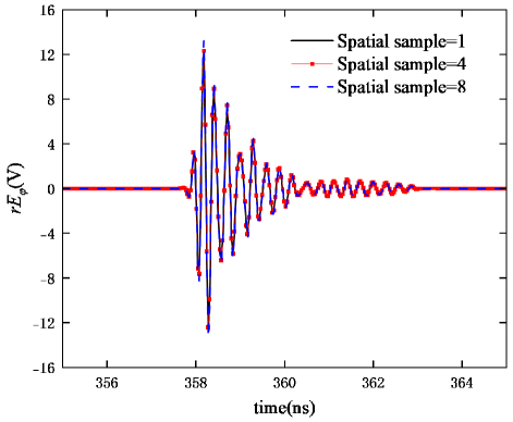
Figure 9: Comparison of far-fields by different spatial samples.
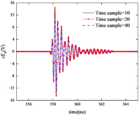
Figure 10: Comparison of far-fields by different time samples.
Table 3: Computation time and maximum relative error of different spatial samples and time samples
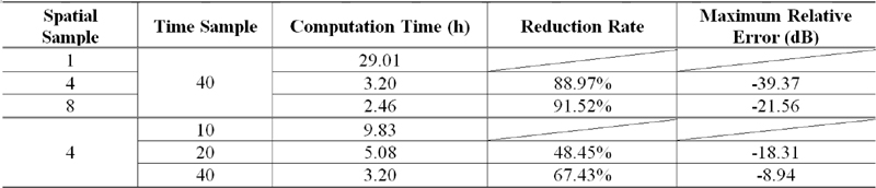
The computation time and maximum relative error for different spatial samples and time samples are presented in Table 3. With an increase in spatial sampling, the maximum relative error remains relatively stable. When the time sample is fixed and the spatial sample is increased from 1 to 8, the computation time decreases from 29.01 hours to 2.46 hours, a reduction of 91.52%. Compared to the result at a spatial sampling of 1, the result at a spatial sampling of 4 exhibits a maximum relative error of -21.56 dB. When the spatial sample is fixed and the time sample is increased from 10 to 40, the computation time decreases from 9.83 hours to 3.20 hours, which is approximately 1/3.07 of the computation time with a time sample of 10. The maximum relative error is -8.94 dB in this case. This indicates that as the spatial and time sample increases, the increase in error is minimal, while there is a significant reduction in computation time, effectively enhancing the computational efficiency of the hybrid algorithm.
Figure 11 presents the corresponding results obtained from commercial software CST. Compared to the result obtained using the sparse sampling optimization method with a spatial sample of 4 and a time sample of 40, the two results are in good agreement. The CST software computed this example with a total grid count of 1.8610, utilizing GPU acceleration, and the entire computation process took 35.8 hours. In contrast, the proposed hybrid algorithm generates 906315 cells in the FDTD computation region and 2616 triangular patches in the TDPO region, achieving a total computation time of 2.46 hours.
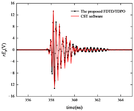
Figure 11: Comparison of transient far-field computed by CST and the proposed FDTD/TDPO.
The method proposed in this paper does not consider the impact of hardware on computation speed and accuracy. Therefore, all methods in the paper were executed on the same computer configuration, detailed as follows: Windows 10 operating system, Intel(R) Xeon(R) 8360Y CPU @ 2.40 GHz 3.50 GHz processor and 1.0 TB RAM. If the size of the parabolic antenna continues to increase, the CST software would be unable to perform transient radiation simulation, whereas the proposed algorithm is not subject to such limitations.
IV. CONCLUSION
This paper presents an optimization algorithm based on the FDTD/TDPO hybrid method, which samples at intervals in the spatial and time domains. The proposed approach preserves the advantages of the hybrid algorithm by segmenting computation regions for composite objects computation, while addressing the issue of slow computation caused by excessive computation load. Numerical validation demonstrates that this optimization significantly enhances computational efficiency without appreciably compromising accuracy, thereby highlighting the reliability and efficiency of the algorithm.
ACKNOWLEDGMENT
This work was supported by the National Key Research and Development Program of China under No. 2020YFA0709800, the National Natural Science Foundations of China under No. 62122061 and the Shaanxi Natural Science Basic Research Project of Shaanxi Science and Technology Office under No. 2023-JC-QN-0673.
REFERENCES
[1] W. Chen, L. Wang, Z. Wu, M. Fang, Q. Deng, A. Wang, Z. Huang, X. Wu, L. Guo, and L. Yang, “Study on the electromagnetic scattering characteristics of high-speed target with non-uniform plasma via the FCC-FDTD method,” IEEE Trans. Antennas Propagat., vol. 70, no. 7, pp. 5744-5757, July 2022.
[2] A. G. Voronovich and V. U. Zavorotny, “The transition from weak to strong diffuse radar bistatic scattering from rough ocean surface,” IEEE Trans. Antennas Propagat., vol. 65, no. 11, pp. 6029-6034, Nov. 2017.
[3] B. Dong, J. Jia, Z. Li, G. Li, J. Shi, H. Wang, N. Chi, and J. Zhang, “Photonic-based flexible integrated sensing and communication with multiple targets detection capability for $w$-band fiber-wireless network,” IEEE Trans. Microwave Theory Techn., pp. 1-14, 2024.
[4] G.-Y. Zhu, W.-D. Li, W. E. I. Sha, H.-X. Zhou, and W. Hong, “A pre-splitting Green’s function based hybrid fast algorithm for multiscale problems,” Applied Computational Electromagnetics Society (ACES) Journal, pp. 652-666, Feb. 2024.
[5] Y. Liang and L. X. Guo, “A study of composite scattering characteristics of movable/rotatable targets and a rough sea surface using an efficient numerical algorithm,” IEEE Trans. Antennas Propagat., vol. 69, no. 7, pp. 4011-4019, July 2021.
[6] C. Ma, Y. Wen, J. Zhang, and D. Zhang, “A hybrid 3-D-ADI-TDPE/DGTD method for multiscale target echo simulation in large-scale complex environments,” IEEE Trans. Microwave Theory Techn., vol. 71, no. 3, pp. 997-1008, Mar. 2023.
[7] X. Wang, S.-X. Gong, J. Ma, and C.-F. Wang, “Efficient analysis of antennas mounted on large-scale complex platforms using hybrid AIM-PO technique,” IEEE Trans. Antennas Propagat., vol. 62, no. 3, pp. 1517-1523, Mar. 2014.
[8] H. Mai, J. Chen, and A. Zhang, “A hybrid algorithm based on FDTD and HIE-FDTD methods for simulating shielding enclosure,” IEEE Trans. Electromagn. Compat., vol. 60, no. 5, pp. 1393-1399, Oct. 2018.
[9] S. Zuo, Z. Lin, Z. Yue, D. Garcia Donoro, Y. Zhang, and X. Zhao, “An efficient parallel hybrid method of FEM-MLFMA for electromagnetic radiation and scattering analysis of separated objects,” Applied Computational Electromagnetics Society (ACES) Journal, vol. 35, no. 10, pp. 1127-1136, Dec. 2020.
[10] K. S. Yee, “Numerical solution of initial boundary value problems involving maxwell’s equations in isotropic media,” IEEE Trans. Antennas Propagat., vol. 14, no. 3, pp. 302-307, May 1966.
[11] E.-Y. Sun and W. V. T. Rusch, “Time-domain physical-optics,” IEEE Transactions on Antennas and Propagation, vol. 42, no. 1, pp. 9-15, 1994.
[12] F. Le Bolzer, R. Gillard, J. Citerne, V. F. Hanna, and M. F. Wong, “An hybrid formulation combining FDTD and TDPO,” in IEEE Antennas and Propagation Society International Symposium. 1998 Digest. Antennas: Gateways to the Global Network. Held in conjunction with: USNC/URSI National Radio Science Meeting, Atlanta, GA, pp. 952-955, 1998.
[13] L.-X. Yang, D.-B. Ge, and B. Wei, “FDTD/TDPO hybrid approach for analysis of the EM scattering of combinative objects,” PIER, vol. 76, pp. 275-284, 2007.
[14] X. Zhu, J. Wang, Z. Chen, L. Cai, and T. Liang, “Hybrid PFDTD-PTDPO method for computing transient far-fields of single reflector,” in 2012 International Conference on Microwave and Millimeter Wave Technology (ICMMT), Shenzhen, China, pp. 1-4, May 2012.
[15] O. M. Ramahi, “Near- and far-field calculations in FDTD simulations using Kirchhoff surface integral representation,” IEEE Transactions on Antennas and Propagation, vol. 45, no. 5, pp. 753-759, 1997.
[16] A. Taflove and S. C. Hagness, Computational Electromagnetics: The Finite-Difference Time-Domain Method, 3rd ed. Boston, MA: Artech House, 2005.
BIOGRAPHIES

Linxi Wang was born in Hubei, China, in 1993. She received the B.S. degree in engineering electronic science and technology from the Xi’an Liaotung University, Xi’an, China, in 2015 and the M.S. degree in microelectronics from the Xi’an Jiao University, Xi’an, China, in 2018. She is currently working toward the Ph.D. degree in electromagnetic field and microwave technology at the school of Information and Communications Engineering, Xi’an Liaotung University, Xi’an, China. Her current research interests include computational electromagnetics and antenna designs.

Juan Chen was born in Chongqing, China. She received the Ph.D. degree from Xi’an Jiaotong University, Xi’an, China, in 2008, in electromagnetic field and microwave technology. She is currently working in Xi’an Jiaotong University, Xi’an, China, as a professor. Her research interests include computational electromagnetics and microwave device design.
ACES JOURNAL, Vol. 40, No. 3, 176–184
doi: 10.13052/2025.ACES.J.400302
© 2025 River Publishers