Sparse Array Optimization Based on Modified Particle Swarm Optimization and Orthogonal Matching Pursuit
Daren Li and Qiang Guo
College of Information and Communication Engineering
Harbin Engineering University, Harbin, 150001, China
lidaren@hrbeu.edu.cn, guoqiang@hrbeu.edu.cn
Submitted On: October 5, 2024; Accepted On: May 27, 2025
ABSTRACT
This paper addresses the low degree of freedom in optimization, primarily attributed to the conventional antenna array optimization methods that solely focus on the optimization of element positions, without considering the influence of element excitations. To address this issue, a sparse array optimization method is proposed based on modified Particle Swarm Optimization (PSO) algorithm and Orthogonal Matching Pursuit (OMP). This method simultaneously optimizes both the element positions and excitations to achieve the desired pattern. Initially, the compressive sensing principle is employed to establish a compressive sensing optimization model for the antenna array. Subsequently, OMP is utilized to simultaneously optimize the element positions and excitations within the antenna array. An improved PSO algorithm is then applied to iteratively update the obtained parameters, thereby further enhancing the peak sidelobe level. Experimental results demonstrate that the proposed algorithm can achieve satisfactory optimization performance.
Index Terms: Compressive sensing, orthogonal matching pursuit, particle swarm optimization algorithm, sparse array antenna.
I. INTRODUCTION
As the radio technology continues to advance, antennas have played a pivotal role in various applications such as communications, remote sensing, navigation, and radar, profoundly influencing every aspect of social life and national defense and military affairs. As the device for receiving and transmitting electromagnetic waves [1], antennas play an irreplaceable role in radio communication systems. The optimization of array antenna deployment is a crucial step in radio communication systems. To enhance performance and meet system requirements, researchers conduct optimizations of array structures by analyzing the relationship between antenna array performance and its geometric configuration [2, 3]. When the spacing between array elements adheres to certain constraints, mutual coupling among elements can be effectively reduced. Nevertheless, this often triggers the issue of grating lobes. Consequently, researchers have embarked on optimizing sparse array antenna technologies. Sparse array antennas, characterized by a smaller number of elements, offer advantages of higher degrees of freedom and broader optimization space [4], attracting extensive research and applications.
In recent years, several studies on sparse array synthesis have attempted to achieve a certain pattern definition with the minimum number of antenna elements by optimizing the excitation coefficients and positions of individual antenna elements. Pinchera et al. proposed a deterministic iterative method for synthesizing isophoric radiation patterns of aperiodic arrays with arbitrary upper limits, which can scan over a wide angle range without violating the sidelobe level constraints [5]. To address the problem of array structure design, Cui et al. introduced a novel Consensus Penalty Dual Decomposition (CPDD) method based on the concept of consensus computing. CPDD utilizes a virtual star topology network, where the central node corresponds to the global variable and each edge node corresponds to a single beam synthesis task. In the outer loop, the algorithm collects excitation vector information from the edge nodes through the central node, then integrates the information to obtain a better co-array structure [6]. Xia and Zhang proposed a new method for synthesizing sparse arrays with discrete phase constraints using Mixed-Integer Programming (MIP). The proposed method optimizes antenna positions and amplitude/phase excitations under given discrete phase constraints [7].
Existing literature on sparse array antenna optimization can be broadly categorized into global optimization [8, 9, 10, 11, 12, 13], matrix pencil method (MPM) [14, 15], and compressed sensing-based array optimization algorithms [16, 17, 18, 19]. Moreover, the intuitionistic fuzzy toolbox based on fuzzy divergence calculation will allow for more effective modeling of the implicit uncertainties and trade-offs in array optimization[20]. Global optimization algorithms transform the synthesis problem into a binary optimization problem, systematically exploring the solution space to find the global optimal solution or a solution close to it. These algorithms are particularly suitable for optimization problems with complex, non-convex objective functions, effectively addressing the nonlinear optimization challenges in sparse arrays. Among them, evolutionary algorithms such as the Genetic Algorithm (GA) [8, 10], Particle Swarm Optimization (PSO) [11], and Differential Evolution (DE) [12, 13] have demonstrated the best performance. However, these algorithms are characterized by high computational complexity. The MPM [14, 15] can be applied to the synthesis of non-uniform arrays. By performing matrix transformations on the signals from the array antenna, MPM efficiently estimates signal sources, making it particularly effective in sparse arrays. MPM can simultaneously optimize the number of elements, element positions, and excitations in a sparse array, allowing the synthesis of sparse arrays to no longer be limited to minimizing the peak sidelobe level by optimizing element positions (and sometimes element excitations) given a fixed number of elements. This opens up new research directions for the synthesis and design of sparse arrays. Nevertheless, the complex matrix operations involved in the MPM algorithm lead to challenges in terms of high computational complexity and implementation difficulty.
Compressed Sensing (CS) technology was introduced in 2006, primarily targeting the solution of sparse signal problems. Research on the application of compressive sensing in array antennas started relatively late. Professor L. Carin from Duke University was the first to theoretically analyze the connection between random sparse arrays and compressive sensing, proving that random sparse arrays are a special case of compressive sensing [21]. The ELEDIA Research Center at the University of Trento in Italy has established a dedicated research group to explore the application of compressive sensing in the field of sparse array antennas, and they have achieved preliminary research results [22]. Experimental results have verified the potential and advantages of applying compressive sensing to the synthesis of sparse array antennas. The emergence of the CS paradigm [17] has significantly advanced the design of sparse arrays. By applying CS techniques to array antenna synthesis, sparse solutions for array antennas are sought. CS-based optimization methods for array antennas effectively reduce the number of array elements, thereby lowering the cost of array construction. Convex optimization [18] minimizes the number of elements by optimizing the weights of each element, converting the solution of the norm into that of the norm, and incorporating certain decision criteria. [19] proposes an algorithm combining Multi-Objective Particle Swarm Optimization (MOPSO) with convex optimization. Through optimization of sparse circular arrays, this algorithm suppresses grating lobes, significantly enhancing the recognizability of the main beam and improving the optimization efficiency of the algorithm. However, these methods overlook the influence of element positions on optimizing array antennas. Furthermore, it is easy for the use of optimization algorithms to get stuck in local optima during the search for global optimal solutions.
To address this, this paper proposes a joint array optimization algorithm based on the Modified Particle Swarm Optimization (MPSO) and Orthogonal Matching Pursuit (OMP), which is applied to both linear arrays and concentric circular arrays. Firstly, the optimization of linear arrays is achieved. With the main beamwidth fixed, the element positions and excitations are optimized. The results show that compared to other algorithms, this proposed algorithm can achieve a lower Peak Side-Lobe Level (PSLL). PSLL refers to the ratio of the maximum value in the sidelobes to the maximum value in the main lobe, and it is an important indicator for evaluating antenna performance, typically expressed in decibels (dB). Generally, radar systems require extremely low sidelobe levels to meet anti-interference requirements and effectively perform target search. Therefore, this parameter is often used as one of the optimization criteria in array synthesis. Secondly, considering the complexity of the array antenna model, the proposed algorithm is further applied to concentric circular arrays. By solving for the excitations of continuous current loops, relevant information about discrete elements can be obtained. According to the simulation results, under the premise of a fixed main beamwidth, although the number of required elements slightly increases, there is a significant improvement in reducing the PSLL.
The structure of this paper is organized as follows: Section II presents the proposed algorithm and model. Section III conducts simulations and analyses of the proposed algorithm, along with a comparative analysis with existing sparse array optimization algorithms. Section IV summarizes and concludes the paper.
II. METHOD DESCRIPTION
A. Array structure model
1. Linear array
As shown in Fig. 1, there are array elements symmetrically distributed on both sides of the axis, with a spacing of between adjacent elements. The directional pattern, as a direct representation of an antenna’s radiation characteristics, can be used to determine the antenna’s directional properties. It not only depicts the spatial distribution of energy when the antenna emits electromagnetic waves but also characterizes the spatial filtering characteristics when receiving electromagnetic waves. Based on the obtained directional pattern, the parameters of the main lobe and side lobes can be determined. Based on the superposition principle, the directional pattern function expression of this linear array is
| (1) |
where represents the excitation of the th element, , is the wavelengths, is the position of the th element, is the signal elevation angle, and . When the element factor , , and when each element adopts equal amplitude and phase excitation (let ), then (1) can be simplified as
| (2) |
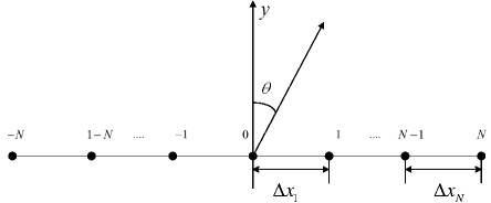
Figure 1: A symmetric linear array with elements.
2. Concentric Ring Array
The Concentric Ring Array (CRA) is composed of multiple concentric circles, with its array elements located on the circles under certain constraints. Its structure is shown in Fig. 2. Assuming there are circles, the radius of the th circle is , and its pattern is shown in (3)
| (3) |
where is the excitation weight of the th ring, and the array element positions are , , , . When , i.e., the excitation of each array element is fixed, (3) can be transformed into (4)
| (4) |
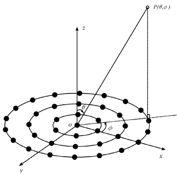
Figure 2: Concentric ring array structure.
For a concentric ring array with uniformly distributed array elements, if the spacing between adjacent array elements in the th ring is , then, given the radius of the ring, the number of array elements in that ring is
| (5) |
where is the defined minimum spacing between array elements, and it is assumed that the spacing between adjacent array elements is not greater than . Then, the number of array elements on the ring should satisfy
| (6) |
When the total number of concentric ring arrays is , then it needs to satisfy
| (7) |
When this model imposes constraints on the total number of array elements, i.e., satisfying (7), controlling the total number of array elements becomes a critical issue. It is necessary to ensure that the total number of array elements remains constant during the optimization process while also ensuring a reasonable distribution of array elements on each ring. [23] proposes a method of linearly weighting the number of array elements, comparing linear models with Gaussian models, and ultimately derives a relationship between the radius of the array elements and the proportion of the total number of array elements, as shown in (8)
| (8) |
where represents the full array occupancy ratio of the number of array elements in the th ring, is the radius of the th concentric ring. , , and are three constants, which can be solved according to the optimization results in the known literature. After determining the full array occupancy ratio, the number of array elements on each ring can be determined
| (9) |
B. Modified Particle Swarm Optimization
The PSO algorithm is combined with adaptive mutation and crossover operations, where the mutation vector is influenced by the individual optimal vector. This process not only maintains the diversity of the population during the iteration process but also ensures that the information of high-quality particles is not destroyed. Adaptive mutation can intervene when the population gets trapped in a local optimum by randomly changing the position or velocity of some particles, enabling them to escape the current optimal region and explore other under-explored areas. The flow of the proposed MPSO algorithm is as follows:
Taking the concentric circular array as an example, suppose the aperture of the concentric circular array is , the minimum spacing between adjacent rings is , the minimum spacing between array elements in the same ring is , the number of populations is , where is the minimum interval between rings to meet the requirements of the array antenna, and is the margin of the rings to form the original mapping vector. Then, the radius of the rings can be expressed as
| (10) |
When the total number of array elements is fixed, the number of elements on each ring can be determined by (8) and (9). According to (10), the value of its peak sidelobe level is related to . Based on the obtained initial population, the peak sidelobe level corresponding to any vector in the population can be determined. Based on the merits of the obtained results, the partial optimal solution and the globally optimal solution are determined. Optimizing can reduce the search space from to , accelerating the search speed and facilitating the acquisition of the optimal solution.
Based on the characteristics of the PSO algorithm, during each iteration process, the position and velocity variables are updated according to the obtained information, as follows
| (11) |
| (12) |
where and are acceleration factors, with being the individual learning factor for each particle and being the social learning factor for particles. represents the position vector corresponding to the individual extremum of the th swarm, and represents the position vector corresponding to the global optimum . is the inertia factor, which is non-negative. In this paper, a linearly decreasing inertia weight is adopted.
| (13) |
where represents the maximum number of iterations, and indicates the current iteration number. stands for the initial weight, for the final weight, and . During the iteration process, the inertia weight decreases linearly from to . At the initial stage of iteration, the inertia weight is larger, which leads to stronger global search capability; as the number of iterations increases, the inertia weight gradually decreases, which facilitates the algorithm’s precise search in local areas. The obtained and need to satisfy the following formula
| (14) |
This paper adopts adaptive mutation, and the generated mutation vector is as follows
| (15) |
where represents the position vector corresponding to the global optimal solution during the th iteration. are distinct positive integers in , and none of them are equal to the target vector index .
To increase the diversity of disturbance variables, a crossover operation is introduced. Define the test variable as
| (16) |
| (17) |
where is the crossover operator, represents the th estimated value generated from a set of random numbers between . denotes a randomly selected integer, used to ensure that at least one set of parameters can undergo crossover.
Calculate the fitness function to determine whether can become a member of the next generation. Compare the fitness of vector in the experiment with that of vector in the population, and retain the better one. Then, based on the obtained population, update the individual optimal and global optimal solutions, and proceed to the next iteration until the specified conditions are met.
The flowchart of this algorithm is shown in Fig. 3.

Figure 3: Flow chart of MPSO.
C. Optimization of linear array by MPSO-OMP
For sparse linear arrays, their array structure is simple, and it is often difficult to obtain the desired radiation characteristics by optimizing only the array element positions. Moreover, the degree of freedom for position optimization is low, resulting in limited optimization of peak sidelobe levels. Therefore, this section utilizes the OMP algorithm to simultaneously optimize the positions and excitations of the array elements in the linear array, and combines the proposed MPSO algorithm to iteratively update the obtained parameters, which is conducive to achieving better peak sidelobe levels. The algorithm flow is as follows:
For a linear array with array elements, its pattern function is as follows
| (18) |
From the above equation, it can be seen that the two vectors that affect its pattern function are the array element positions and the array element excitations. In the process of joint optimization, the obtained PSLL is used as the performance evaluation index. Assuming that the minimum spacing between adjacent array elements is , and the desired main beam is , where is the shaping area of the main beam, the optimization model can be expressed as
| (19) |
Initialize the position vector , and establish an OMP sparse recovery model based on the desired shaping main beam . Solve for the corresponding array element excitation vector of the position vector .
| (20) |
Based on , the corresponding PSLL is solved, and the individual best value and the global optimal value in the population are determined. The obtained results are then carried over to the nextiteration.
Utilize the velocity information of the PSO algorithm to update its position information. Generate a mutation vector through adaptive mutation based on the global optimal solution, and select the results. The specific operation process is detailed in II.B.
Substitute the obtained array element positions into (20), with the peak sidelobe level as the optimization objective, and determine the array element excitations under the condition that the main beam does not change significantly. Based on the results obtained, update the individual optimal solution and the global optimal solution, and carry the results into the next iteration process. When the number of iterations reaches the maximum iteration count, stop the iteration, and the global optimal solution obtained is the optimal result from the optimization process.
D. Optimization of concentric ring array by MPSO-OMP
Unlike linear arrays, concentric ring arrays have more parameters that affect the radiation pattern, including element positions, ring radii, the number of elements, and element excitations. To achieve a lower peak sidelobe level, this section conducts a multi-variable joint optimization of concentric circular arrays with uniformly distributed elements to obtain better radiation characteristics. For the concentric circular array structure shown in Fig. 2, its radiation pattern can be represented by (4). The radiation pattern function of the concentric circular array can be equivalently substituted using the zeroth-order Bessel series, and the substituted formula is shown below
| (21) | |||
As can be seen from, (21) the radiation pattern function at this time only depends on the radiation angle , the ring radius , and the excitation matrix . This section also adopts the equivalent form of the Bessel series to solve the radiation pattern of the circular array. Similarly, the excitation vector of the continuous current loop is first obtained, and then it is equivalently replaced by discrete elements. The number of elements and excitation amplitudes on the corresponding ring are determined based on minimizing the matching error value. Different from the reconstruction process, for the radius variable in the steering vector , this section does not adopt a small step size similar to that established in the reconstruction process. Instead, it utilizes a set of random numbers that meet the requirements, which are randomly generated during the initialization process of the MPSO algorithm. The specific steps are as follows:
Based on the above description, under the constraint of satisfying the main beam conditions, the optimization process for the concentric circular array mainly consists of two parts. Firstly, the corresponding ring radii and excitation matrices under continuous current loop excitation are obtained. Then, the discrete elements are used for equivalent substitution to determine the number of uniformly distributed elements and the excitation amplitudes of each ring. The optimization model can be composed of two parts, as shown (22) and (23)
| (22) |
| (23) |
For this model, the initial values of the ring radii are first determined. When the minimum spacing between adjacent rings is constrained to , and the array aperture is , the initialization of the radii for rings can be set as follows
| (24) |
Based on the initialized vector, the OMP algorithm is utilized to solve for the excitation matrix of the continuous current loop, with the obtained element radii as known quantities, under the condition of a fixed main beam. Through calculations based on the obtained information, the individual optimal solution and the global optimal solution within the population can be determined.
The initialization results are brought into the iteration process to update the particle information. To increase population diversity, mutation and selection operations are performed on relevant particles, with the specific operational process as described earlier.
The individual optimal solution and global optimal solution are updated based on the obtained results. The criterion for whether to update is to determine if the peak sidelobe level of the obtained result is more optimal, and the particle information corresponding to the lower peak sidelobe level is retained.
After obtaining the optimal solution corresponding to the continuous current loop excitation matrix through iteration, according to (25), the number of uniformly distributed elements on each ring can be determined simply by specifying the total number of elements. Based on the number of elements on each concentric ring, the matching error value between the concentric circular array under discrete element conditions and the continuous current loop excitation can be determined. By finding the number of elements that minimizes matching error value, the equivalent substitution of the continuous current loop can be completed, and the excitation amplitudes of the discrete elements on the rings can be obtained.
| (25) |
III. NUMERICAL EXAMPLES
A. MPSO-OMP optimization for linear array
For sparse linear arrays, their array structure is simple, and it is often difficult to obtain the desired radiation characteristics by optimizing only the element positions. Moreover, the degree of freedom for position optimization is low, limiting the optimization of PSLL. [24] proposes the IGA-EDSPSO algorithm to jointly optimize the element positions and excitations in linear arrays. This algorithm combines Improvements of Genetic Algorithm (IGA) and the modified PSO algorithm. By comparing the results obtained by the hybrid algorithm with those of the two individual algorithms, it is found that the optimization results of the hybrid algorithm are relatively excellent. This section will utilize the MPSO-OMP algorithm to jointly optimize the element positions and excitations in linear arrays. In the simulation process of [24], the array aperture is constrained to , the total number of elements is 17, and the minimum spacing between adjacent elements is . Under these conditions, the IGA-EDSPSO algorithm achieves a PSLL of -26.67 dB, with a corresponding main beam width (FNBW) of 17.4 in the pattern diagram. [25] proposes the IWO-CVX algorithm, which combines CVX technology with Invasive Weed Optimization (IWO) and applies it to the optimization process of sparse linear arrays. The simulation conditions are the same as those for IGA-EDSPSO.
To verify the effectiveness of the proposed algorithm in optimizing sparse linear arrays, the optimization of sparse linear arrays is conducted under the same conditions. The results obtained by this algorithm are compared with those in [24] and [25]. During the optimization process, the main beam width is also constrained to 17.4. First, 10 independent simulation experiments are conducted for the proposed algorithm, with , , , population size , and maximum number of iterations . The convergence curves of the Monte Carlo simulation values obtained from the 10 independent experiments are shown in Fig. 4.
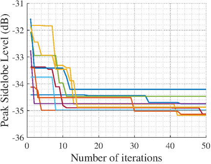
Figure 4: The convergence curves corresponding to the results of the 10 independent experiments.
According to Fig. 4, during the optimization process with a total of 50 iterations, most of the results tend to stabilize after 15 iterations and remain unchanged in the later stages. However, a few results show variations during the 30th to 45th iterations. Although the convergence curves of the obtained results exhibit some fluctuations in the later stages of optimization, the number of iterations is only 50 and, under a limited number of iterations, the results obtained are relatively impressive. The Monte Carlo simulation values, i.e., PSLLs, obtained from the 10 independent experiments are shown in Table 1.
Table 1: PSLLs obtained from 10 independent experiments
| No. | 1 | 2 | 3 | 4 | 5 | 6 | 7 | 8 | 9 | 10 |
| PSLL | 37.45 | 34.98 | 35.17 | 34.74 | 34.74 | 34.98 | 35.13 | 34.21 | 35.14 | 34.87 |
According to Table 1, the optimal PSLL obtained from 10 independent experiments is -35.17 dB, the worst PSLL is -34.21 dB, and the average PSLL is -34.84 dB. Compared with the results obtained by the IGA-EDSPSO algorithm, the optimal PSLL obtained by the MPSO-OMP algorithm is optimized by 8.5 dB, and the worst PSLL is optimized by 7.54 dB, with an optimization ratio of approximately 28.3% to 31.9%. Therefore, taking PSLL as the performance evaluation index and under the condition of the same main beamwidth, the proposed algorithm exhibits significant superiority in optimizing sparse linear arrays compared to the IGA-EDSPSO algorithm. This paper also compares the results with those obtained by the IWO-CVX algorithm proposed in [25]. Under the same conditions, the optimal PSLL obtained by the IWO-CVX algorithm after 10 independent experiments with a maximum number of iterations of 50 is -33.85 dB, and the worst PSLL is -33.62 dB. The results obtained by the proposed algorithm, both optimal and worst PSLL, are superior to those obtained by the IWO-CVX algorithm. Moreover, the worst PSLL obtained by the proposed algorithm is approximately 0.36 dB better than the optimal PSLL obtained by the IWO-CVX algorithm. This result demonstrates that under the condition of the same main beamwidth, the optimization results of the MPSO-OMP for sparse linear arrays are superior to those obtained by the IWO-CVX algorithm, making it more suitable for joint optimization of element positions and element excitations. Figure 5 shows the comparison of the optimal array patterns, and Table 2 presents the excitation amplitudes and element positions obtained from theexperiments.
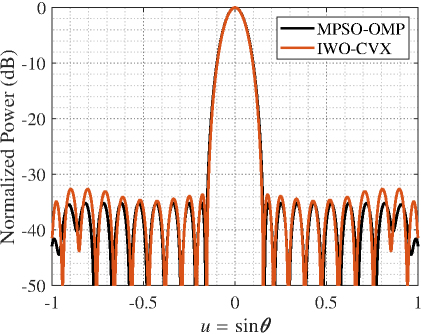
Figure 5: Comparison of optimal array pattern obtained by MPSO-OMP and IWO-CVX.
Table 2: Comparison of joint optimization results for sparse array of array elements
| Element Number | IWO-CVX Optimal Array | MPSO-OMP Worst Array | MPSO-OMP Optimal Array | |||
| Element Positions | Excitation Amplitudes | Element Positions | Excitation Amplitudes | Element Positions | Excitation Amplitudes | |
| 1 | 0 | 0.225 | 0 | 0.155 | 0 | 0.193 |
| 2 | 0.765 | 0.315 | 0.726 | 0.219 | 0.702 | 0.270 |
| 3 | 1.353 | 0.289 | 1.282 | 0.338 | 1.339 | 0.388 |
| 4 | 1.867 | 0.524 | 1.910 | 0.501 | 1.952 | 0.513 |
| 5 | 2.581 | 0.788 | 2.606 | 0.628 | 2.561 | 0.667 |
| 6 | 3.270 | 0.769 | 3.113 | 0.548 | 3.171 | 0.752 |
| 7 | 3.770 | 0.661 | 3.645 | 0.835 | 3.711 | 0.727 |
| 8 | 4.313 | 0.854 | 4.314 | 0.997 | 4.241 | 0.870 |
| 9 | 4.820 | 0.709 | 4.994 | 1 | 4.849 | 1 |
| 10 | 5.383 | 1 | 5.641 | 0.920 | 5.482 | 0.924 |
| 11 | 6.091 | 0.975 | 6.237 | 0.718 | 6.019 | 0.687 |
| 12 | 6.728 | 0.652 | 6.738 | 0.602 | 6.522 | 0.718 |
| 13 | 7.238 | 0.574 | 7.313 | 0.636 | 7.101 | 0.645 |
| 14 | 7.834 | 0.487 | 7.890 | 0.415 | 7.680 | 0.523 |
| 15 | 8.354 | 0.327 | 8.412 | 0.326 | 8.310 | 0.447 |
| 16 | 8.948 | 0.321 | 9.027 | 0.307 | 9.034 | 0.229 |
| 17 | 9.744 | 0.228 | 9.744 | 0.163 | 9.744 | 0.187 |
B. MPSO-OMP optimization for concentric ring array
Chen et al. employ a Modified Genetic Algorithm (MGA) to optimize a concentric ring array, jointly optimizing the array element positions and the number of array elements for a 6-ring array under the condition that the aperture [9]. The experimental results indicate that this algorithm achieves a PSLL of -28.33 dB, with a total of 142 array elements in the array. This paper compares with this algorithm by optimizing the relevant parameters of the concentric ring array under the same aperture width and number of rings, using the peak sidelobe level as the performance evaluation metric for simulation experiments.
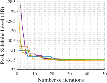
Figure 6: Convergence curves corresponding to the five independent experiments.
To ensure that the main beam correlation coefficient remains unchanged after the experiment, the main beam width is constrained during this simulation process. The main beam width obtained in the pattern generated by the MGA algorithm is 16.9 and, similarly, this paper also constrains the main beam width to 16.9 during the simulation process. Based on the above analysis, the simulation analysis of the concentric ring array using the MPSO-OMP algorithm consists of two parts: first, solving the continuous current loop excitation variables using OMP to determine the ring radii and continuous current loop excitations; second, determining the number of array elements for each ring under a uniform distribution based on the obtained results. This section conducts five independent simulation experiments for the first part of the operation, which are carried out when the population size and there are 50 iterations. The convergence curves obtained from the results are shown in Fig. 6.
As shown in Fig. 6, the algorithm exhibits excellent convergence performance under continuous current loop excitation. Despite only 50 iterations, the results gradually stabilize after the 25th iteration, approaching the final optimized results. Moreover, the results from the five experiments show little variation, all converging around -31.5 dB. Therefore, this paper analyzes the optimal array obtained from the five experiments and determines the number of array elements on the rings based on the relevant continuous current loop excitations and ring radii obtained under these conditions. The normalized continuous current loop excitations and ring radii corresponding to the optimal array are shown inTable 3.
Table 3: Parameters corresponding to the optimal array obtained by MPSO-OMP
| Number of Rings | 1 | 2 | 3 | 4 | 5 | 6 |
| Current Loop Excitation | 0.2434 | 6.271 | 0.9919 | 1 | 0.8384 | 0.9586 |
| Ring Radius | 0.5436 | 1.2703 | 2.0792 | 2.9170 | 3.7587 | 4.7 |
| PSLL (dB) | -31.5445 | |||||
Table 4: Comparison of results obtained by MPSO-OMP and MGA
| Method Number | MGA | MPSO-OMP | |||
| Ring Radius | Number of Elements | Ring Radius | Number of Elements | Excitation Amplitudes | |
| 1 | 0.7604 | 9 | 0.5436 | 7 | 1 |
| 2 | 1.3180 | 16 | 1.2703 | 20 | 0.9019 |
| 3 | 2.0969 | 26 | 2.0792 | 29 | 0.9124 |
| 4 | 2.9305 | 30 | 2.9170 | 32 | 0.8989 |
| 5 | 3.7852 | 27 | 3.7587 | 27 | 0.8931 |
| 6 | 4.7000 | 33 | 4.7000 | 33 | 0.8355 |
| Number of elements | 142 | 149 | |||
| Main beam width | 16.9 | 16.9 | |||
| PSLL (dB) | -28.33 | -31.5445 | |||
By minimizing the matching error as the criterion, the total number of corresponding array elements can be determined, thereby obtaining the number of array elements uniformly distributed on each ring. The results obtained are presented in Table 4 along with the relevant data from the MGA algorithm.
According to Table 4, when the array aperture is , the number of rings is 6, and the main beam width remains consistent, the PSLL obtained by MPSO-OMP is approximately 3.2145 dB lower than the optimal PSLL achieved by the MGA algorithm reported in the literature, demonstrating a significant optimization effect. Although the number of array elements increases by 5, which is about 3.5% of the original array, the PSLL has been greatly improved, thus, the impact of the increased number of array elements can be neglected. The results obtained in this paper correspond to the three-dimensional pattern and array elements as shown in Fig. 7. The comparison of patterns at between the results obtained in this paper and those by MGA is illustrated in Fig. 8.
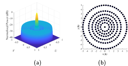
Figure 7: The optimal array’s three-dimensional pattern and element distribution obtained by MPSO-OMP.
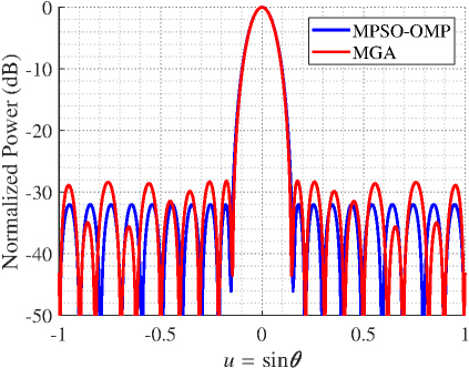
Figure 8: Comparison of directional patterns between results obtained by MPSO-OMP and MGA.
As can be seen from Fig. 8, the MPSO-OMP algorithm can achieve a lower PSLL. This is because MPSO-OMP optimizes the excitation of the array elements in the array by utilizing the OMP sparse recovery principle, while keeping the fitness calculation function unchanged. Although this algorithm can achieve a lower sidelobe level, it requires a relatively large amount of computation and a longer calculation time, making it suitable for antenna systems with high requirements for sidelobe levels.
IV. CONCLUSION
In this paper, the application of compressive sensing-related techniques in the optimization of sparse arrays is investigated. Analyzing both linear arrays and concentric circular arrays, the MPSO-OMP algorithm is proposed for joint optimization of multiple variables, including array element excitations. Firstly, an MPSO algorithm is introduced, incorporating adaptive mutation and crossover operations within the PSO framework. The mutation vector in this process is influenced by the individual best vector, which not only maintains the diversity of the population during iterations but also ensures that the information of high-quality particles is preserved. Furthermore, by integrating the OMP algorithm and making reasonable choices regarding array element excitations, the number of array elements, and the radius of the circular rings, a reduction in the peak sidelobe level is achieved. Simulation results demonstrate that the proposed algorithm can achieve satisfactory optimization performance for array antennasystems.
ACKNOWLEDGMENT
This work was supported in part by the National Natural Science Foundation of China under Grant 62071140.
REFERENCES
[1] R. L. Haupt, Antenna Arrays: A Computational Approach. Hoboken, NJ: Wiley, 2010.
[2] S. A. Hamza and M. G. Amin, “Sparse array design for optimum beamforming using deep learning,” IEEE Transactions on Aerospace and Electronic Systems, vol. 60, no. 1, pp. 133-144, Feb. 2024.
[3] N. Amani, A. Farsaei, S. R. Aghdam, T. Eriksson, M. V. Ivashina, and R. Maaskant, “Sparse array synthesis including mutual coupling for MU-MIMO average capacity maximization,” IEEE Transactions on Antennas and Propagation, vol. 70, no. 8, pp. 6617-6626, Aug. 2022.
[4] M. G. Amin, Sparse Arrays for Radar, Sonar, and Communications. Hoboken, NJ: John Wiley & Sons, pp. i-xxiv, 2024.
[5] D. Pinchera, M. D. Migliore, and G. Panariello, “Isophoric inflating deflating exploration algorithm (I-IDEA) for equal-amplitude aperiodic arrays,” IEEE Transactions on Antennas and Propagation, vol. 70, no. 11, pp. 10405-10416, Nov. 2022.
[6] Z. M. Cui, Q. H. Zhang, J. F. An, Y. Yu, and B. B. Cheng, “Multibeam synthesis for a reconfigurable sparse array via a vew consensus PDD framework,” IEEE Transactions on Antennas and Propagation, vol. 72, no. 2, pp. 1541-1555, Feb. 2024.
[7] D. N. Xia and X. J. Zhang, “Synthesis of sparse arrays with discrete phase constraints via mixed-integer programming,” IEEE Antennas and Wireless Propagation Letters, vol. 23, no. 3, pp. 1030-1034, Mar. 2024.
[8] K. S. Chen, H. Chen, L. Wang, and H. G. Wu, “Modified real GA for the synthesis of sparse planar circular arrays,” IEEE Antennas and Wireless Propagation Letters, vol. 15, pp. 274-277, 2016.
[9] K. S. Chen, Y. Y. Zhu, X. L. Ni, and H. Chen, “Low sidelobe sparse concentric ring arrays optimization using modified GA,” International Journal of Antennas and Propagation, vol. 2015, p. 147247, 2015.
[10] K. S. Chen, Z. S. He, and C. L. Han, “A modified real GA for the sparse linear array synthesis with multiple constraints,” IEEE Transactions on Antennas and Propagation, vol. 54, no. 7, pp. 2169-2173, July 2006.
[11] Y. Li, F. Yang, J. Ouyang, Z. P. Nie, and H. J. Zhou, “Synthesis of nonuniform array antennas using particle swarm optimization,” Electromagnetics, vol. 30, no. 3, pp. 237-245, 2010.
[12] Z. Y. He, K. S. Chen, Z. S. He, and C. L. He, “Sparse circular arrays method based on modified DE algorithm,” Systems Engineering and Electronics, vol. 31, no. 3, p. 497-499, 2009.
[13] K. Du, Z. K. Chen, D. L. Peng, and X. T. Zhu, “Sparse optimization of uniform array based on hybrid mutation differential evolution algorithm,” Modern Radar, vol. 54, no. 7, pp. 2169-2173, July 2006.
[14] Y. H. Liu, Z. P. Nie, and Q. H. Liu, “Reducing the number of elements in a linear antenna array by the matrix pencil method,” IEEE Transactions on Antennas and Propagation, vol. 56, no. 9, pp. 2955-2962, Sep. 2008.
[15] H. O. Shen, B. H. Wang, and X. Li, “Shaped-beam pattern synthesis of sparse linear arrays using the unitary matrix pencil method,” IEEE Antennas and Wireless Propagation Letters, vol. 16, pp. 1098-1101, 2017.
[16] E. J. Candès, J. Romberg, and T. Tao, “Robust uncertainty principles Exact signal reconstruction from highly incomplete frequency information,” IEEE Transactions on Information Theory, vol. 52, no. 2, pp. 489-509, Feb.2006.
[17] E. J. Candès and M. B. Wakin, “An introduction to compressive sampling,” IEEE Signal Processing Magazine, vol. 25, no. 2, pp. 21-30, Mar.2008.
[18] T. Hong, X. P. Shi, and X. S. Liang, “Synthesis of sparse linear array for directional modulation via convex optimization,” IEEE Transactions on Antennas and Propagation, vol. 66, no. 8, pp. 3959-3972, Aug. 2018.
[19] A. H. Cao, H. L. Li, S. L. Ma, J. Tan, and J. J. Zhou, “Sparse circular array pattern optimization based on MOPSO and convex optimization,” in 2015 Asia-Pacific Microwave Conference (APMC), Vols 1-3, 2015.
[20] M. Versaci, G. Angiulli, F. La Foresta, F. Laganà, and A. Palumbo, “Intuitionistic fuzzy divergence for evaluating the mechanical stress state of steel plates subject to bi-axial loads,” Integrated Computer-Aided Engineering, vol. 31, no. 4, pp. 363-379, 2024.
[21] L. Carin, “On the relationship between compressive sensing and random sensor arrays,” IEEE Antennas and Propagation Magazine, vol. 51, no. 5, pp. 72-81, 2009.
[22] G. Oliveri and A. Massa, “Bayesian compressive sampling for pattern synthesis with maximally sparse non-uniform linear arrays,” IEEE Transactions on Antennas and Propagation, vol. 59, no. 2, pp. 467-481, 2011.
[23] K. Chen, Y. Li, and J. Shi, “Optimization of sparse concentric ring arrays for low sidelobe,” International Journal of Antennas and Propagation, vol. 2019, no. 1, pp. 1485075, June 2019.
[24] S. Zhang, S. X. Gong, Y. Guan, P. F. Zhang, and Q. Gong, “A novel IGA-EDSPSO hybrid algorithm for the synthesis of sparse arrays,” Progress in Electromagnetics Research-PIER, vol. 89, pp. 121-134, 2009.
[25] Y. Liu, Y. R. N. Zhang, and S. Gao, “Suppress sideband radiation in time-modulated linear arrays by an effective hybrid algorithm,” in Proceedings of 2020 IEEE 10th International Conference on Electronics Information and Emergency Communication (ICEIEC 2020), pp. 257-260,2020.
BIOGRAPHIES

Daren Li was born in Harbin, Heilongjiang Province, China, in 1990. He received the M.S. degree in shipbuilding and ocean engineering from the College of Shipbuilding Engineering, Harbin Engineering University, Harbin, China, where he is currently working toward the Ph.D. degree in information and communication engineering with Harbin Engineering University of Information and Communication Engineering. His research interests include antenna array synthesis, radar signal processing and target comprehensive identification.

Qiang Guo received the B.S., M.S., and Ph.D. degrees in information and communication engineering from Harbin Engineering University, China, in 1994, 2003, and 2007, respectively. In 2009, he joined the Faculty with the School of Information and Communication Engineering, Harbin Engineering University, where he is currently a Full Professor. His research interests include antenna array synthesis, machine learning, radar signals sorting, and recognition. He is also a Foreign member of the Ukrainian Academy of Engineering, Review Expert of the Science and Technology Commission of the Military Commission, the National Natural Science Foundation of China and Technology Department evaluation expert and the Chinese Institute of Electronics Science and Technology Award evaluation expert.
ACES JOURNAL, Vol. 40, No. 6, 508–519
doi: 10.13052/2024.ACES.J.400603
© 2025 River Publishers