Surface Integral Equations in Computational Electromagnetics: A Comprehensive Overview of Theory, Formulations, Discretization Schemes and Implementations

Parmenion S. Mavrikakis and Olivier J. F. Martin

Nanophotonics and Metrology Laboratory
École Polytechnique Fédérale de Lausanne, CH-1015 Lausanne, Switzerland
parmenion.mavrikakis@epfl.ch, olivier.martin@epfl.ch

Submitted On: October 9, 2024; Accepted On: April 17, 2025

ABSTRACT

Computational electromagnetics based on surface integral equations provides accurate and efficient solutions for three-dimensional electromagnetic scattering problems in the frequency domain. In this review paper, we first introduce a complete and detailed theoretical analysis of the surface integral equation method, including different properties of the corresponding integral operators and equations. Using a pedagogical approach that should appeal to electrical engineers, we provide a systematic and comprehensive derivation of the different formulations found in the literature and discuss their advantages and pitfalls. Additionally, we provide a mathematical overview of the corresponding function spaces that clarifies the importance of correctly combining basis and testing functions and we examine the various aspects of discretization schemes, such as the Green’s function singularity subtraction and the application of different testing methods. Moreover, we assess alternative formulations and discretization procedures and draw particular conclusions about them, by comparing numerous examples and results from previously published works. Finally, we provide a detailed discussion on numerical solvers and approaches.

Index Terms: Basis function, Buffa-Christiansen function, Calderon preconditioner, discretization, electromagnetic scattering, fast solvers, formulation, Green’s function, half-Rao-Wilton-Glisson function, high-performance computing, integral equation, integral operator, low frequency breakdown, Method of Moments, Rao-Wilton-Glisson function, singularity subtraction, surface integral equation, testing function, testing method, Trintinalia-Ling functions.

I. INTRODUCTION

For many decades, computational electromagnetics has been playing a crucial role both in academia and in industry, to investigate a plethora of phenomena [1, 2, 3, 4, 5, 6]. Indeed, analytical expressions for electromagnetic scattering problems exist only for objects with very specific shapes. For scattering, Mie theory can be used only to model analytically homogeneous, coated, or multilayered spheres and infinite cylinders [7]. The treatment of scatterers with more complex geometries requires the use of accurate numerical techniques.

A very popular technique used for modeling scattering objects is the discrete dipole approximation (DDA), which approximates the scatterer by a finite array of polarizable point dipoles [8, 9], but presents enormous computational costs for large objects [10]. Numerical techniques that are based on differential formulations like the finite element method (FEM) [11, 12, 13] and the finite-difference time-domain (FDTD) [14, 15, 16] have sparse matrices in the final linear system, which is a significant advantage since they can use efficient storage and solver algorithms with better performances. Nevertheless, the discretization of the whole computational domain (including the surrounding medium) and the existence of spurious modes represent some major concerns for these approaches [17].

Volume integral equations (VIEs) use the integral form of Maxwell’s equations [18]. Contrary to differential techniques, only the discretization of the scatterer’s domain is needed [19]. The surrounding is not discretized since its effect is intrinsically included in the formulation. Also, VIEs can be used to model inhomogeneous materials. However, an important disadvantage of VIEs is that they involve densely populated matrices [20].

Surface integral equations (SIEs), are very efficient because they only require the discretization of the scatterer’s surface, thus presenting a significantly smaller number of unknowns compared to VIEs [21]. However, they are limited to piecewise homogeneous materials since they use the Green’s function of a homogeneous region. The SIE method is a widely used numerical approach for analyzing electromagnetic scattering in metallic, dielectric, and composite metallic-dielectric structures [22]. SIEs can be formulated in many different ways for the same electromagnetic problem. Thus, one may wonder what is the best formulation to use? Some of the most popular SIE formulations for impenetrable scatterers are the electric field integral equation (EFIE), magnetic field integral equation (MFIE) and combined-field integral equation (CFIE) [23]. For penetrable objects the most used formulations are the Poggio-Miller-Chang-Harrington-Wu-Tsai (PMCHWT) [24] and Müller [25]. In the 1970s and 1980s many numerical approaches were introduced for solving the aforementioned equations, initially for rotationally symmetric objects [23, 26, 27], and subsequently for arbitrarily shaped three-dimensional (3D) objects [28, 29, 30]. SIEs can be categorized into the Fredholm integral equations of the first and the second kinds [31]. EFIE and PMCHWT equations are both of the first kind. MFIE and Müller equations belong to the second kind. The first kind of surface integral equations present a superior numerical accuracy compared to the second kind, while the latter show better performance regarding iterative solutions and convergence [32]. Hence, identifying a specific formulation as the most optimal is not straightforward. The main reason behind this trade-off between accuracy and iterative solution convergence has been proven to originate from the improper testing of the second kind of formulations [33, 34]. Hence, in every problem, the discretization scheme (selection of basis and testing functions) and the SIE formulation must be selected carefully, since the numerical accuracy and efficiency of the solution are heavily affected by this formulation-discretization combination.

In this review, we present the theoretical analysis of a general electromagnetic problem that leads to different SIE formulations. We discuss the integral operators, the integral equations and the different formulations. Moreover, we delve into the various components of a discretization scheme, such as the singularity subtraction and the utilization of different basis and testing functions, by providing also a mathematical overview of function spaces to explain the significance of combining basis and testing functions properly. Furthermore, we go through several results from various published works, in order to compare different formulations and discretization procedures, so that we can draw specific conclusions about them alone and also about their combination. Finally, we provide a detailed discussion on numerical solvers and approaches.

II. THEORETICAL FRAMEWORK

A. Scattering problems

Consider Fig. 1, where a scatterer is placed in a homogeneous background. The scatterer is of arbitrary shape and consists of piecewise homogeneous media. Every region is a domain ${\mathrm{\Omega }}_i$ with a constant electric permittivity ${\epsilon }_i$ and magnetic permeability ${\mu }_i$. The time dependence $e^{-j\omega t}$ is used throughout.

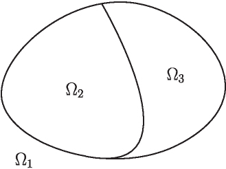
Figure 1: Scatterer in a homogeneous background ${\mathrm{\Omega }}_1$.

For each domain,

$$\nabla \times \nabla \times {\mathbf{E}}_i(\mathbf{r})-k_i^2{\mathbf{E}}_i(\mathbf{r})=j\omega {\mu }_i{\mathbf{J}}_i(\mathbf{r}),$$

(1)

where $k_i=\omega \sqrt{{\epsilon }_i{\mu }_i}$. The Dyadic Green’s function ${\overline{\mathbf{G}}}_i(\mathbf{r},{\mathbf{r}}^{\prime })$ solves the equation [35]

$$\nabla \times \nabla \times {\overline{\mathbf{G}}}_i(\mathbf{r},{\mathbf{r}}^{\prime })-k_i^2{\overline{\mathbf{G}}}_i(\mathbf{r},{\mathbf{r}}^{\prime })=\overline{\mathbf{1}}\delta \left(\mathbf{r}-{\mathbf{r}}^{\prime }\right).$$

(2)

The multiplication of (1) with ${\overline{\mathbf{G}}}_i(\mathbf{r},{\mathbf{r}}^{\prime })$ from the right and (2) with ${\overline{\mathbf{E}}}_i\left(\mathbf{r}\right)$ from the left gives

	$$\nabla \times \nabla \times {\mathbf{E}}_i(\mathbf{r})\cdot {\overline{\mathbf{G}}}_i(\mathbf{r},{\mathbf{r}}^{\prime })-$$
	$${\mathbf{E}}_i(\mathbf{r})\cdot \nabla \times \nabla \times {\overline{\mathbf{G}}}_i(\mathbf{r},{\mathbf{r}}^{\prime })=$$
	$$j\omega {\mu }_i{\mathbf{J}}_i(\mathbf{r})\cdot {\overline{\mathbf{G}}}_i(\mathbf{r},{\mathbf{r}}^{\prime })-{\mathbf{E}}_i(\mathbf{r})\delta \left(\mathbf{r}-{\mathbf{r}}^{\prime }\right).$$		(3)

Integrating (3) over ${\mathrm{\Omega }}_i$ and using the following relation [36]

	$$\nabla \cdot ([\nabla \times \mathbf{E}(\mathbf{r})]\times \overline{\mathbf{G}}(\mathbf{r},{\mathbf{r}}^{\prime })+$$
	$$\mathrm{\hspace{1em}}\mathit{\hspace{1em}\hspace{1em}\hspace{1em}}\mathbf{E}(\mathbf{r})\times [\nabla \times \overline{\mathbf{G}}(\mathbf{r},{\mathbf{r}}^{\prime })])=$$		(4)
	$$\nabla \times \nabla \times \mathbf{E}(\mathbf{r})\cdot \overline{\mathbf{G}}(\mathbf{r},{\mathbf{r}}^{\prime })-\mathbf{E}(\mathbf{r})\cdot \nabla \times \nabla \times \overline{\mathbf{G}}(\mathbf{r},{\mathbf{r}}^{\prime }),$$

gives

	${\displaystyle {\int }_{{\mathrm{\Omega }}_i}}\mathrm{d}V\nabla \cdot ($	$\left[\nabla \times {\mathbf{E}}_i(\mathbf{r})\right]\times {\overline{\mathbf{G}}}_i(\mathbf{r},{\mathbf{r}}^{\prime })+$
		${\mathbf{E}}_i(\mathbf{r})\times [\nabla \times {\overline{\mathbf{G}}}_i(\mathbf{r},{\mathbf{r}}^{\prime })])=$
	${\mathbf{E}}_i^{\text{inc}}\left({\mathbf{r}}^{\prime }\right)-$	$\{\begin{array}{cc}{\mathbf{E}}_i\left({\mathbf{r}}^{\prime }\right),\hfill & {\mathbf{r}}^{\prime }\in {\mathrm{\Omega }}_i\hfill \\ \kappa \left({\mathbf{r}}^{\prime }\right){\mathbf{E}}_i\left({\mathbf{r}}^{\prime }\right),\hfill & {\mathbf{r}}^{\prime }\in \partial {\mathrm{\Omega }}_i\hfill \\ 0,\hfill & {\mathbf{r}}^{\prime }\notin {\mathrm{\Omega }}_i\hfill \end{array},$		(5)

where

	${\mathbf{E}}_i^{\mathrm{inc}}\left({\mathbf{r}}^{\prime }\right)$	$=j\omega {\mu }_i{\displaystyle {\int }_{{\mathrm{\Omega }}_i}}dV{\mathbf{J}}_i(\mathbf{r})\cdot {\overline{\mathbf{G}}}_i(\mathbf{r},{\mathbf{r}}^{\prime })$
		$=j\omega {\mu }_i{\displaystyle {\int }_{{\mathrm{\Omega }}_i}}dV{\overline{\mathbf{G}}}_i({\mathbf{r}}^{\prime },\mathbf{r})\cdot {\mathbf{J}}_i(\mathbf{r}),$		(6)

is the incident electric field intensity generated by the current density ${\mathbf{J}}_i(\mathbf{r})$ inside ${\mathrm{\Omega }}_i$. Regarding the transposition of the Dyadic Green’s function [37], ${\overline{\mathbf{G}}}_i{(\mathbf{r},{\mathbf{r}}^{\prime })}^T={\overline{\mathbf{G}}}_i({\mathbf{r}}^{\prime },\mathbf{r})$. Next, by using Gauss’ theorem, the following surface integral emerges

	${\displaystyle {\int }_{\partial {\mathrm{\Omega }}_i}}\mathrm{d}S{\widehat{\mathbf{n}}}_i\cdot ($	$\left[\nabla \times {\mathbf{E}}_i(\mathbf{r})\right]\times {\overline{\mathbf{G}}}_i(\mathbf{r},{\mathbf{r}}^{\prime })+$
		${\mathbf{E}}_i(\mathbf{r})\times [\nabla \times {\overline{\mathbf{G}}}_i(\mathbf{r},{\mathbf{r}}^{\prime })])=$
	${\mathbf{E}}_i^{\text{inc}}\left({\mathbf{r}}^{\prime }\right)-$	$\{\begin{array}{ccc}{\mathbf{E}}_i\left({\mathbf{r}}^{\prime }\right),\hfill & {\mathbf{r}}^{\prime }\in {\mathrm{\Omega }}_i\hfill & \\ \kappa \left({\mathbf{r}}^{\prime }\right){\mathbf{E}}_i\left({\mathbf{r}}^{\prime }\right),\hfill & {\mathbf{r}}^{\prime }\in \partial {\mathrm{\Omega }}_i\hfill & \\ 0,\hfill & {\mathbf{r}}^{\prime }\notin {\mathrm{\Omega }}_i\hfill & \end{array},$		(7)

where ${\widehat{\mathbf{n}}}_i$ is the unit normal vector on $\partial {\mathrm{\Omega }}_i$ with direction from the inside to the outside of ${\mathrm{\Omega }}_i$. By using the time-harmonic nature of the different field quantities, the kernel of the integral becomes [37]

	${\widehat{\mathbf{n}}}_i(\mathbf{r})\cdot \left[\nabla \times {\mathbf{E}}_i(\mathbf{r})\right]\times {\overline{\mathbf{G}}}_i(\mathbf{r},{\mathbf{r}}^{\prime })=$
	${\widehat{\mathbf{n}}}_i(\mathbf{r})\times \left[\nabla \times {\mathbf{E}}_i(\mathbf{r})\right]\cdot {\overline{\mathbf{G}}}_i(\mathbf{r},{\mathbf{r}}^{\prime })=$
	$j\omega {\mu }_i{\overline{\mathbf{G}}}_i({\mathbf{r}}^{\prime },\mathbf{r})\cdot \left[{\widehat{\mathbf{n}}}_i(\mathbf{r})\times {\mathbf{H}}_i(\mathbf{r})\right],$		(8)

and with the use of

$${\left[\nabla \times {\overline{\mathbf{G}}}_i(\mathbf{r},{\mathbf{r}}^{\prime })\right]}^{\mathbf{T}}=-\nabla \times {\overline{\mathbf{G}}}_i({\mathbf{r}}^{\prime },\mathbf{r}),$$

(9)

the second kernel term becomes

	${\widehat{\mathbf{n}}}_i(\mathbf{r})\cdot {\mathbf{E}}_i(\mathbf{r})\times \left[\nabla \times {\overline{\mathbf{G}}}_i(\mathbf{r},{\mathbf{r}}^{\prime })\right]$	$=$
	$\left[{\widehat{\mathbf{n}}}_i(\mathbf{r})\times {\mathbf{E}}_i(\mathbf{r})\right]\cdot \left[\nabla \times {\overline{\mathbf{G}}}_i(\mathbf{r},{\mathbf{r}}^{\prime })\right]$	$=$
	$-\left[\nabla \times {\overline{\mathbf{G}}}_i({\mathbf{r}}^{\prime },\mathbf{r})\right]\cdot \left[{\widehat{\mathbf{n}}}_i(\mathbf{r})\times {\mathbf{E}}_i(\mathbf{r})\right]$	$\mathrm{\hspace{0.17em}}.$		(10)

Finally, by introducing the surface electric and magnetic current densities

	${\mathbf{J}}_{s,i}(\mathbf{r})$	$={\widehat{\mathbf{n}}}_i(\mathbf{r})\times {\mathbf{H}}_i(\mathbf{r})$		(11)
	${\mathbf{M}}_{s,i}(\mathbf{r})$	$=-{\widehat{\mathbf{n}}}_i(\mathbf{r})\times {\mathbf{E}}_i(\mathbf{r}),$		(12)

where ${\widehat{\mathbf{n}}}_i(\mathbf{r})$ is the unit normal vector of $\partial {\mathrm{\Omega }}_i$ towards the outer side of ${\mathrm{\Omega }}_i$. Equation (7) becomes [18]

	${\eta }_i\left[j{k}_i{\displaystyle {\int }_{\partial {\mathrm{\Omega }}_i}}d{S}^{\prime }{\overline{\mathbf{G}}}_i(\mathbf{r},{\mathbf{r}}^{\prime })\cdot {\mathbf{J}}_{s,i}\left({\mathbf{r}}^{\prime }\right)\right]+$
	${\displaystyle {\int }_{\partial {\mathrm{\Omega }}_i}}d{S}^{\prime }\left[{\nabla }^{\prime }\times {\overline{\mathbf{G}}}_i(\mathbf{r},{\mathbf{r}}^{\prime })\right]\cdot {\mathbf{M}}_{s,i}\left({\mathbf{r}}^{\prime }\right)=$
	${\mathbf{E}}_i^{\mathrm{inc}}\left(\mathbf{r}\right)-\{\begin{array}{ccc}{\mathbf{E}}_i\left(\mathbf{r}\right),\hfill & \mathbf{r}\in {\mathrm{\Omega }}_i\hfill & \\ \kappa \left(\mathbf{r}\right){\mathbf{E}}_i\left(\mathbf{r}\right),\hfill & \mathbf{r}\in \partial {\mathrm{\Omega }}_i\hfill & \\ 0,\hfill & \mathbf{r}\notin {\mathrm{\Omega }}_i\hfill & \end{array},$		(13)

where $\mathbf{r}$ and ${\mathbf{r}}^{\prime }$ have been swapped. Also, $\kappa \left(\mathbf{r}\right)=1-\mathrm{\Omega }\left(\mathbf{r}\right)/4\pi$, where $\mathrm{\Omega }\left(\mathbf{r}\right)$ is the solid angle subtended by the observation point $\mathbf{r}$ [18]. For locally smooth surfaces $\mathrm{\Omega }\left(\mathbf{r}\right)=2\pi$, thus $\kappa \left(\mathbf{r}\right)=1/2$.

A similar analysis can be applied to the case of the magnetic field [38]. Starting from the following equation

$$\nabla \times \nabla \times {\mathbf{H}}_i(\mathbf{r})-k_i^2{\mathbf{H}}_i(\mathbf{r})=\nabla \times {\mathbf{J}}_i(\mathbf{r}).$$

(14)

By identifying the incident magnetic field intensity as

	${\mathbf{H}}_i^{\mathrm{inc}}\left({\mathbf{r}}^{\prime }\right)$	$={\displaystyle {\int }_{{\mathrm{\Omega }}_i}}dV{\mathbf{J}}_i(\mathbf{r})\cdot \left[{\nabla }^{\prime }\times {\overline{\mathbf{G}}}_i(\mathbf{r},{\mathbf{r}}^{\prime })\right]$
		$={\displaystyle {\int }_{{\mathrm{\Omega }}_i}}dV{\overline{\mathbf{G}}}_i({\mathbf{r}}^{\prime },\mathbf{r})\cdot \left[\nabla \times {\mathbf{J}}_i(\mathbf{r})\right],$		(15)

an analogous equation is derived

	${\eta }_i^{-1}\left[j{k}_i{\displaystyle {\int }_{\partial {\mathrm{\Omega }}_i}}d{S}^{\prime }{\overline{\mathbf{G}}}_i(\mathbf{r},{\mathbf{r}}^{\prime })\cdot {\mathbf{M}}_{s,i}\left({\mathbf{r}}^{\prime }\right)\right]-$
	${\displaystyle {\int }_{\partial {\mathrm{\Omega }}_i}}d{S}^{\prime }\left[{\nabla }^{\prime }\times {\overline{\mathbf{G}}}_i(\mathbf{r},{\mathbf{r}}^{\prime })\right]\cdot {\mathbf{J}}_{s,i}\left({\mathbf{r}}^{\prime }\right)=$
	${\mathbf{H}}_i^{\text{inc}}\left(\mathbf{r}\right)-\{\begin{array}{ccc}{\mathbf{H}}_i\left(\mathbf{r}\right),\hfill & \mathbf{r}\in {\mathrm{\Omega }}_i\hfill & \\ \kappa \left(\mathbf{r}\right){\mathbf{H}}_i\left(\mathbf{r}\right),\hfill & \mathbf{r}\in \partial {\mathrm{\Omega }}_i\hfill & \\ 0,\hfill & \mathbf{r}\notin {\mathrm{\Omega }}_i\hfill & \end{array}.$		(16)

After the solution of the above integral equations, the currents can be used to calculate the fields at any position $\mathbf{r}\in {\mathrm{\Omega }}_i$, as follows

	${\mathbf{E}}_i\left(\mathbf{r}\right)=$	${\mathbf{E}}_i^{\text{inc}}\left(\mathbf{r}\right)-$
		${\eta }_i\left[j{k}_i{\displaystyle {\int }_{\partial {\mathrm{\Omega }}_i}}d{S}^{\prime }{\overline{\mathbf{G}}}_i(\mathbf{r},{\mathbf{r}}^{\prime })\cdot {\mathbf{J}}_{s,i}\left({\mathbf{r}}^{\prime }\right)\right]-$
		${\displaystyle {\int }_{\partial {\mathrm{\Omega }}_i}}d{S}^{\prime }\left[{\nabla }^{\prime }\times {\overline{\mathbf{G}}}_i(\mathbf{r},{\mathbf{r}}^{\prime })\right]\cdot {\mathbf{M}}_{s,i}\left({\mathbf{r}}^{\prime }\right),$		(17)
	${\mathbf{H}}_i\left(\mathbf{r}\right)=$	${\mathbf{H}}_i^{\text{inc}}\left(\mathbf{r}\right)-$
		${\eta }_i^{-1}\left[j{k}_i{\displaystyle {\int }_{\partial {\mathrm{\Omega }}_i}}d{S}^{\prime }{\overline{\mathbf{G}}}_i(\mathbf{r},{\mathbf{r}}^{\prime })\cdot {\mathbf{M}}_{s,i}\left({\mathbf{r}}^{\prime }\right)\right]+$
		${\displaystyle {\int }_{\partial {\mathrm{\Omega }}_i}}d{S}^{\prime }\left[{\nabla }^{\prime }\times {\overline{\mathbf{G}}}_i(\mathbf{r},{\mathbf{r}}^{\prime })\right]\cdot {\mathbf{J}}_{s,i}\left({\mathbf{r}}^{\prime }\right).$		(18)

B. Boundary conditions

As illustrated in Fig. 2, we assume the existence of two domains ${\mathrm{\Omega }}_1$ and ${\mathrm{\Omega }}_2$ with different media, and a boundary $\partial \mathrm{\Omega }=\partial {\mathrm{\Omega }}_1\cap \partial {\mathrm{\Omega }}_2$. Maxwell’s equations require that the tangential components of the electric and magnetic fields are continuous across the boundary $\partial \mathrm{\Omega }$, as depicted in the following equations, where $\mathbf{r}\in \partial \mathrm{\Omega }$:

	$\widehat{\mathbf{n}}(\mathbf{r})\times {\mathbf{H}}_1\left(\mathbf{r}\right)$	$=-\widehat{\mathbf{n}}(\mathbf{r})\times {\mathbf{H}}_2\left(\mathbf{r}\right),$		(19)
	$-\widehat{\mathbf{n}}(\mathbf{r})\times {\mathbf{E}}_1\left(\mathbf{r}\right)$	$=\widehat{\mathbf{n}}(\mathbf{r})\times {\mathbf{E}}_2\left(\mathbf{r}\right),$		(20)

where $\widehat{\mathbf{n}}(\mathbf{r})={\widehat{\mathbf{n}}}_1(\mathbf{r})$ is the the unit normal vector of $\partial \mathrm{\Omega }$ pointing towards ${\mathrm{\Omega }}_2$ and ${\widehat{\mathbf{n}}}_2(\mathbf{r})=-\widehat{\mathbf{n}}(\mathbf{r})$, as shown in Fig. 2. Thus, when it comes to the surface electric and magnetic current densities on $\partial {\mathrm{\Omega }}_1$ and $\partial {\mathrm{\Omega }}_2$, the relation between them for $\mathbf{r}\in \partial \mathrm{\Omega }$ is

	${\mathbf{J}}_{s,1}\left(\mathbf{r}\right)$	$=-{\mathbf{J}}_{s,2}\left(\mathbf{r}\right),$		(21)
	${\mathbf{M}}_{s,1}\left(\mathbf{r}\right)$	$=-{\mathbf{M}}_{s,2}\left(\mathbf{r}\right).$		(22)

The above relations between surface current densities play a key role not only for the theoretical formulation, but also for its discretization.

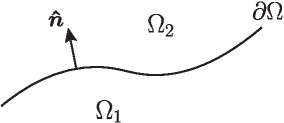
Figure 2: Boundary between the domains ${\mathrm{\Omega }}_1$, ${\mathrm{\Omega }}_2$, and definition of the normal $\widehat{\mathbf{n}}(\mathbf{r})$.

III. SURFACE INTEGRAL FORMULATIONS

A. Integral operators

Formally, a linear integral equation can be written

$$ℒ\left\{\mathbf{s}\right\}=\mathbf{R},$$

(23)

where $ℒ$ is the integral (linear) operator, $\mathbf{s}$ is the unknown quantity (the electric and magnetic surface current densities) and $\mathbf{R}$ is the known quantity (the excitation). The surface integral operator

$$ℒ\left\{\mathbf{s}\right\}\left(\mathbf{r}\right)={\int }_{\partial \mathrm{\Omega }}d{S}^{\prime }K(\mathbf{r},{\mathbf{r}}^{\prime })\mathbf{s}\left({\mathbf{r}}^{\prime }\right)$$

(24)

includes a kernel $K(\mathbf{r},{\mathbf{r}}^{\prime })$ and the integral runs over a boundary $\partial \mathrm{\Omega }$ of the geometry.

The linear integral operator can be categorized according to its singularity. If the singularity order is less than the integral’s dimension, then the operator is weakly singular [39]. An example of such an operator is the following

$${ℒ}_w\left\{\mathbf{s}\right\}\left(\mathbf{r}\right)={\int }_{\partial \mathrm{\Omega }}d{S}^{\prime }\frac{1}{|\mathbf{r}-{\mathbf{r}}^{\prime }|}\mathbf{s}\left({\mathbf{r}}^{\prime }\right).$$

(25)

In this case, as $|\mathbf{r}-{\mathbf{r}}^{\prime }|\to 0$, the kernel becomes singular. Its singularity dimension is equal to 1. However, since we are integrating over the 2D surface $\partial \mathrm{\Omega }$, the integral’s dimension is equal to 2. Thus, this is a weak (or mild) singularity, and the integral remains finite. Additionally, a weakly singular integral operator ${ℒ}_w$ is bounded and maps a function to a smoother one, because its range space is reduced by one order relative to its original domain [40]. Furthermore, the spectrum of a bounded operator accumulates to a constant and, in the special case that it accumulates to zero, the integral operator is said to be compact [41]. Regarding the previously presented example, the integral operator ${ℒ}_w$ is compact, meaning its eigenvalues (in spectral terms) accumulate to zero, and the operator tends to smooth the function it acts upon. If the singularity order is equal to or larger than the integral’s dimension, then the operator is singular or hyper-singular, respectively. A typical hyper-singular example arises from increasing the power of the kernel’s denominator, as follows

$${ℒ}_h\left\{\mathbf{s}\right\}\left(\mathbf{r}\right)={\int }_{\partial \mathrm{\Omega }}d{S}^{\prime }\frac{1}{{|\mathbf{r}-{\mathbf{r}}^{\prime }|}^3}\mathbf{s}\left({\mathbf{r}}^{\prime }\right).$$

(26)

In this scenario, as $|\mathbf{r}-{\mathbf{r}}^{\prime }|\to 0$, the kernel becomes singular. However, its singularity dimension is equal to 3 and it is larger than the integral’s dimension. Operators with (hyper-)singular kernels can lead to the appearance of an unbounded operator, with a spectrum that tends to go to infinity [42]. In the following sections we identify the integral operators that appear in (13) and (16) of the aforementioned analysis.

1. $𝒟$ operator

In (13) and (16) there is the linear integral operator

$${𝒟}_i\left\{𝒳\right\}\left(\mathbf{r}\right)=j{k}_i{\int }_{\partial {\mathrm{\Omega }}_i}d{S}^{\prime }{\overline{\mathbf{G}}}_i(\mathbf{r},{\mathbf{r}}^{\prime })\cdot 𝒳\left({\mathbf{r}}^{\prime }\right),$$

(27)

where $𝒳\left(\mathbf{r}\right)$ can be the surface electric current density ${\mathbf{J}}_{s,i}\left(\mathbf{r}\right)$ or the surface magnetic current density ${\mathbf{M}}_{s,i}\left(\mathbf{r}\right)$. By taking into consideration that

	${\overline{\mathbf{G}}}_i(\mathbf{r},{\mathbf{r}}^{\prime })$	$=\left(\overline{\mathbf{1}}+{\displaystyle \frac{\nabla \nabla }{k_i^2}}\right){\displaystyle \frac{e^{j{k}_i\left|\mathbf{r}-{\mathbf{r}}^{\prime }\right|}}{4\pi \left|\mathbf{r}-{\mathbf{r}}^{\prime }\right|}}$
		$=\left(\overline{\mathbf{1}}+{\displaystyle \frac{\nabla \nabla }{k_i^2}}\right)G_i(\mathbf{r},{\mathbf{r}}^{\prime }),$		(28)

equation (27) can lead to the following calculations

	${𝒟}_i\left\{𝒳\right\}\left(\mathbf{r}\right)=$	$j{k}_i{\displaystyle {\int }_{\partial {\mathrm{\Omega }}_i}}d{S}^{\prime }{\overline{\mathbf{G}}}_i(\mathbf{r},{\mathbf{r}}^{\prime })\cdot 𝒳\left({\mathbf{r}}^{\prime }\right)$
	$=$	$j{k}_i{\displaystyle {\int }_{\partial {\mathrm{\Omega }}_i}}d{S}^{\prime }{G}_i(\mathbf{r},{\mathbf{r}}^{\prime })𝒳\left({\mathbf{r}}^{\prime }\right)-$		(29)
		${\displaystyle \frac{1}{j{k}_i}}\nabla {\displaystyle {\int }_{\partial {\mathrm{\Omega }}_i}}d{S}^{\prime }{G}_i(\mathbf{r},{\mathbf{r}}^{\prime }){\nabla }_s^{\prime }\cdot 𝒳\left({\mathbf{r}}^{\prime }\right).$

2. $𝒦$ operator

In (13) and (16) we can also identify the linear integral operator

$${𝒦}_i\left\{𝒳\right\}\left(\mathbf{r}\right)={\int }_{\partial {\mathrm{\Omega }}_i}d{S}^{\prime }\left[{\nabla }^{\prime }\times {\overline{\mathbf{G}}}_i(\mathbf{r},{\mathbf{r}}^{\prime })\right]\cdot 𝒳\left({\mathbf{r}}^{\prime }\right),$$

(30)

which, with the use of equation ${\nabla }^{\prime }\times {\overline{\mathbf{G}}}_i(\mathbf{r},{\mathbf{r}}^{\prime })={\nabla }^{\prime }{G}_i(\mathbf{r},{\mathbf{r}}^{\prime })\times \overline{\mathbf{1}}$, can be further written as follows

	${𝒦}_i\left\{𝒳\right\}\left(\mathbf{r}\right)$	$={\displaystyle {\int }_{\partial {\mathrm{\Omega }}_i}}d{S}^{\prime }\left[{\nabla }^{\prime }\times {\overline{\mathbf{G}}}_i(\mathbf{r},{\mathbf{r}}^{\prime })\right]\cdot 𝒳\left({\mathbf{r}}^{\prime }\right)$
		$={\displaystyle {\int }_{\partial {\mathrm{\Omega }}_i}}d{S}^{\prime }\left[{\nabla }^{\prime }{G}_i(\mathbf{r},{\mathbf{r}}^{\prime })\right]\times 𝒳\left({\mathbf{r}}^{\prime }\right).$		(31)

B. Integral equations

As mentioned in section I., two different kinds of integral equations exist. The integral equations of the first kind,

$${ℒ}_1\left\{\mathbf{s}\right\}=\mathbf{R},$$

(32)

and those of the second kind,

$$\left({ℒ}_2+ℐ\right)\left\{\mathbf{s}\right\}=\mathbf{R},$$

(33)

where $ℐ\left\{\mathbf{s}\right\}$ is the identity operator [41]. An integral equation of the first kind has a unique solution if the linear integral operator is coercive and one-to-one [43]. For an integral equation of the second kind, a unique solution exists when the operator ${ℒ}_2+ℐ$ is one-to-one and the integral operator ${ℒ}_2$ is compact [43]. In general, an integral equation with an operator of the form $ℒ+𝒦$ has a unique solution if $ℒ+𝒦$ is one-to-one, $ℒ$ is compact, and $𝒦$ is a bounded operator with a bounded inverse [42, 43, 44]. Hence, in order to have unique solutions, in (32) the linear integral operator should not be compact, and in (33) it should not be unbounded [42].

According to the calculations of the previous sections, (13) and (16) can be rewritten on a (locally) smooth surface $\partial {\mathrm{\Omega }}_i$ as follows

	${\eta }_i{𝒟}_i\left\{{\mathbf{J}}_{s,i}\right\}\left(\mathbf{r}\right)$	$+{𝒦}_i\left\{{\mathbf{M}}_{s,i}\right\}\left(\mathbf{r}\right)=$
	${\mathbf{E}}_i^{\mathrm{inc}}\left(\mathbf{r}\right)$	$-{\displaystyle \frac{1}{2}}{\mathbf{E}}_i\left(\mathbf{r}\right),\mathbf{r}\in \partial {\mathrm{\Omega }}_i,$		(34)
	$-{𝒦}_i\left\{{\mathbf{J}}_{s,i}\right\}\left(\mathbf{r}\right)$	$+{\eta }_i^{-1}{𝒟}_i\left\{{\mathbf{M}}_{s,i}\right\}\left(\mathbf{r}\right)=$
	${\mathbf{H}}_i^{\mathrm{inc}}\left(\mathbf{r}\right)$	$-{\displaystyle \frac{1}{2}}{\mathbf{H}}_i\left(\mathbf{r}\right),\mathbf{r}\in \partial {\mathrm{\Omega }}_i.$		(35)

The electric and magnetic fields can then be split into components parallel and perpendicular to the boundary $\partial {\mathrm{\Omega }}_i$:

	${\mathbf{E}}_i\left(\mathbf{r}\right)=$	$\left[{\mathbf{E}}_i\left(\mathbf{r}\right)\times {\widehat{\mathbf{n}}}_i\left(\mathbf{r}\right)\right]\times {\widehat{\mathbf{n}}}_i\left(\mathbf{r}\right)+$
		$\left[{\widehat{\mathbf{n}}}_i\left(\mathbf{r}\right)\cdot {\mathbf{E}}_i\left(\mathbf{r}\right)\right]{\widehat{\mathbf{n}}}_i\left(\mathbf{r}\right),$		(36)
	${\mathbf{H}}_i\left(\mathbf{r}\right)=$	$\left[{\mathbf{H}}_i\left(\mathbf{r}\right)\times {\widehat{\mathbf{n}}}_i\left(\mathbf{r}\right)\right]\times {\widehat{\mathbf{n}}}_i\left(\mathbf{r}\right)+$
		$\left[{\widehat{\mathbf{n}}}_i\left(\mathbf{r}\right)\cdot {\mathbf{H}}_i\left(\mathbf{r}\right)\right]{\widehat{\mathbf{n}}}_i\left(\mathbf{r}\right).$		(37)

Using the boundary conditions and the continuity equations leads to the following expressions for (34) and (35):

	$${\eta }_i𝒟\left\{{\mathbf{J}}_{s,i}\right\}\left(\mathbf{r}\right)+𝒦\left\{{\mathbf{M}}_{s,i}\right\}\left(\mathbf{r}\right)-\frac{1}{2}{\widehat{\mathbf{n}}}_i\left(\mathbf{r}\right)\times {\mathbf{M}}_{s,i}\left(\mathbf{r}\right)$$
	$$+j\frac{{\eta }_i}{2k_i}\left[{\nabla }_s\cdot {\mathbf{J}}_{s,i}\left(\mathbf{r}\right)\right]{\widehat{\mathbf{n}}}_i\left(\mathbf{r}\right)={\mathbf{E}}_i^{\mathrm{inc}}\left(\mathbf{r}\right),\mathbf{r}\in \partial {\mathrm{\Omega }}_i,$$		(38)
	$$-𝒦\left\{{\mathbf{J}}_{s,i}\right\}\left(\mathbf{r}\right)+{\eta }_i^{-1}𝒟\left\{{\mathbf{M}}_{s,i}\right\}\left(\mathbf{r}\right)+\frac{1}{2}{\widehat{\mathbf{n}}}_i\left(\mathbf{r}\right)\times {\mathbf{J}}_{s,i}\left(\mathbf{r}\right)$$
	$$+j\frac{1}{2{\eta }_i{k}_i}\left[{\nabla }_s\cdot {\mathbf{M}}_{s,i}\left(\mathbf{r}\right)\right]{\widehat{\mathbf{n}}}_i\left(\mathbf{r}\right)={\mathbf{H}}_i^{\mathrm{inc}}\left(\mathbf{r}\right),\mathbf{r}\in \partial {\mathrm{\Omega }}_i.$$		(39)

Equation (38) is the electric field integral equation (EFIE) and (39) the magnetic field integral equation (MFIE).

Formulations that use either the EFIE or the MFIE for the solution of a scattering problem often lead to internal resonances, which produce inaccurate results, especially at a resonance frequency of the scatterer [45]. To avoid this major problem, different combinations of the EFIE and MFIE have been proposed. Surface integral equation formulations, which are free of internal resonances, can thus be obtained by summing, with appropriate coefficients, the EFIEs and the MFIEs for all computational domains, which leads to a final matrix system of combined integral equations that are solved simultaneously [46]. A conventional approach to derive SIE formulations involves the tangential traces of the EFIE and MFIE representations, along with the boundary conditions. Thus, two categories of SIE formulations are produced. The N-Formulations are produced by combining the following tangential components

	${(\mathrm{N}-\mathrm{EFIE})}_i:$	$\mathrm{\hspace{0.17em}}{\left[\widehat{\mathbf{n}}\left(\mathbf{r}\right)\times (\mathrm{EFIE})\right]}_{\partial {\mathrm{\Omega }}_i},$		(40)
	${(\mathrm{N}-\mathrm{MFIE})}_i:$	$\mathrm{\hspace{0.17em}}{\left[\widehat{\mathbf{n}}\left(\mathbf{r}\right)\times (\mathrm{MFIE})\right]}_{\partial {\mathrm{\Omega }}_i},$		(41)

and the T-Formulations consist of

	$(\mathrm{T}-\mathrm{EFIE}):$	$\mathrm{\hspace{0.17em}}{\left[-\widehat{\mathbf{n}}\left(\mathbf{r}\right)\times \widehat{\mathbf{n}}\left(\mathbf{r}\right)\times (\mathrm{EFIE})\right]}_{\partial {\mathrm{\Omega }}_i},$		(42)
	$(\mathrm{T}-\mathrm{MFIE}):$	$\mathrm{\hspace{0.17em}}{\left[-\widehat{\mathbf{n}}\left(\mathbf{r}\right)\times \widehat{\mathbf{n}}\left(\mathbf{r}\right)\times (\mathrm{MFIE})\right]}_{\partial {\mathrm{\Omega }}_i},$		(43)

where $\widehat{\mathbf{n}}\left(\mathbf{r}\right)$ is the outward unit normal vector on the closed surface $\partial {\mathrm{\Omega }}_i$.

C. N-Formulations

Consider a boundary $\partial \mathrm{\Omega }$ between two adjacent domains ${\mathrm{\Omega }}_{\mathrm{\ell }}$ and ${\mathrm{\Omega }}_m$. The selection $\widehat{\mathbf{n}}\left(\mathbf{r}\right)={\widehat{\mathbf{n}}}_{\mathrm{\ell }}\left(\mathbf{r}\right)$ is made, where ${\widehat{\mathbf{n}}}_{\mathrm{\ell }}\left(\mathbf{r}\right)$ is the normal unit vector of $\partial \mathrm{\Omega }$ towards ${\mathrm{\Omega }}_m$. Then, N-EFIE and N-MFIE take the following forms in the domains ${\mathrm{\Omega }}_{\mathrm{\ell }}$ and ${\mathrm{\Omega }}_m$:

	${(\mathrm{N}-\mathrm{EFIE})}_{\mathrm{\ell }}:$
	$\mathrm{\hspace{0.17em}}+{\eta }_{\mathrm{\ell }}{𝒟}_{\mathrm{\ell }}^n\left\{{\mathbf{J}}_{s,\mathrm{\ell }}\right\}\left(\mathbf{r}\right)+\left({𝒦}_{\mathrm{\ell }}^n+{\displaystyle \frac{ℐ}{2}}\right)\left\{{\mathbf{M}}_{s,\mathrm{\ell }}\right\}\left(\mathbf{r}\right)=$
	$\widehat{\mathbf{n}}\left(\mathbf{r}\right)\times {\mathbf{E}}_{\mathrm{\ell }}^{\mathrm{inc}}\left(\mathbf{r}\right),$		(44)
	${(\mathrm{N}-\mathrm{EFIE})}_m:$
	$\mathrm{\hspace{0.17em}}-{\eta }_m{𝒟}_m^n\left\{{\mathbf{J}}_{s,\mathrm{\ell }}\right\}\left(\mathbf{r}\right)-\left({𝒦}_m^n-{\displaystyle \frac{ℐ}{2}}\right)\left\{{\mathbf{M}}_{s,\mathrm{\ell }}\right\}\left(\mathbf{r}\right)=$
	$\widehat{\mathbf{n}}\left(\mathbf{r}\right)\times {\mathbf{E}}_m^{\mathrm{inc}}\left(\mathbf{r}\right),$		(45)
	${(\mathrm{N}-\mathrm{MFIE})}_{\mathrm{\ell }}:$
	$\mathrm{\hspace{0.17em}}-\left({𝒦}_{\mathrm{\ell }}^n+{\displaystyle \frac{ℐ}{2}}\right)\left\{{\mathbf{J}}_{s,\mathrm{\ell }}\right\}\left(\mathbf{r}\right)+{\eta }_{\mathrm{\ell }}^{-1}{𝒟}_{\mathrm{\ell }}^n\left\{{\mathbf{M}}_{s,\mathrm{\ell }}\right\}\left(\mathbf{r}\right)=$
	$\widehat{\mathbf{n}}\left(\mathbf{r}\right)\times {\mathbf{H}}_{\mathrm{\ell }}^{\mathrm{inc}}\left(\mathbf{r}\right),$		(46)
	${(\mathrm{N}-\mathrm{MFIE})}_m:$
	$\mathrm{\hspace{0.17em}}+\left({𝒦}_m^n-{\displaystyle \frac{ℐ}{2}}\right)\left\{{\mathbf{J}}_{s,\mathrm{\ell }}\right\}\left(\mathbf{r}\right)-{\eta }_m^{-1}{𝒟}_m^n\left\{{\mathbf{M}}_{s,\mathrm{\ell }}\right\}\left(\mathbf{r}\right)=$
	$\widehat{\mathbf{n}}\left(\mathbf{r}\right)\times {\mathbf{H}}_m^{\mathrm{inc}}\left(\mathbf{r}\right),$		(47)

where $ℐ$ is the identity operator and

	${𝒟}_i^n\left\{𝒳\right\}\left(\mathbf{r}\right)$	$=\widehat{\mathbf{n}}\left(\mathbf{r}\right)\times {𝒟}_i\left\{𝒳\right\}\left(\mathbf{r}\right),$		(48)
	${𝒦}_i^n\left\{𝒳\right\}\left(\mathbf{r}\right)$	$=\widehat{\mathbf{n}}\left(\mathbf{r}\right)\times {𝒦}_i\left\{𝒳\right\}\left(\mathbf{r}\right).$		(49)

Different N-Formulations can then be obtained by combining the previous equations with different coefficients, as shown below

	$m_{\mathrm{\ell }}^N{(\mathrm{N}-\mathrm{MFIE})}_{\mathrm{\ell }}$	$+m_m^N{(\mathrm{N}-\mathrm{MFIE})}_m,$		(50)
	$e_{\mathrm{\ell }}^N{(\mathrm{N}-\mathrm{EFIE})}_{\mathrm{\ell }}$	$+e_m^N{(\mathrm{N}-\mathrm{EFIE})}_m.$		(51)

The most popular formulation of this kind is mN-Müller [47] with coefficients

$$m_{\mathrm{\ell }}^N=\frac{{\mu }_{\mathrm{\ell }}}{{\mu }_m+{\mu }_{\mathrm{\ell }}},m_m^N=\frac{{\mu }_m}{{\mu }_m+{\mu }_{\mathrm{\ell }}},$$

(52)

and

$$e_{\mathrm{\ell }}^N=\frac{{\epsilon }_{\mathrm{\ell }}}{{\epsilon }_m+{\epsilon }_{\mathrm{\ell }}},e_m^N=\frac{{\epsilon }_m}{{\epsilon }_m+{\epsilon }_{\mathrm{\ell }}}.$$

(53)

The N-Müller (with coefficients: $m_{\mathrm{\ell }}^N={\mu }_{\mathrm{\ell }}$, $m_m^N={\mu }_m$, $e_{\mathrm{\ell }}^N={\epsilon }_{\mathrm{\ell }}$, $e_m^N={\epsilon }_m$) [25] and mN-Müller [47] formulations have very fast rates of convergence when iterative solvers are used [48]. This happens because of the identity operator that appears on the diagonal of the system matrix. Thus, these formulations present a low condition number and fast convergence [48]. However, there are losses in terms of accuracy with the use of divergence-conforming basis functions of the lowest order, which will be discussed in section IV.B..

D. T-Formulations

T-Formulations are a linear combination of the T-EFIE (42) and the T-MFIE (43). Again, consider a boundary $\partial \mathrm{\Omega }$ between two adjacent domains ${\mathrm{\Omega }}_{\mathrm{\ell }}$ and ${\mathrm{\Omega }}_m$. The selection $\widehat{\mathbf{n}}\left(\mathbf{r}\right)={\widehat{\mathbf{n}}}_{\mathrm{\ell }}\left(\mathbf{r}\right)$ is made, where ${\widehat{\mathbf{n}}}_{\mathrm{\ell }}\left(\mathbf{r}\right)$ is the normal unit vector of $\partial \mathrm{\Omega }$ towards ${\mathrm{\Omega }}_m$. Then, T-EFIE and T-MFIE take the following forms in the domains ${\mathrm{\Omega }}_{\mathrm{\ell }}$ and ${\mathrm{\Omega }}_m$:

		${(\mathrm{T}-\mathrm{EFIE})}_{\mathrm{\ell }}:$
		$\mathrm{\hspace{0.17em}}+{\eta }_{\mathrm{\ell }}{𝒟}_{\mathrm{\ell }}^t\left\{{\mathbf{J}}_{s,\mathrm{\ell }}\right\}\left(\mathbf{r}\right)+\left({𝒦}_{\mathrm{\ell }}^t-{\displaystyle \frac{{ℐ}_n}{2}}\right)\left\{{\mathbf{M}}_{s,\mathrm{\ell }}\right\}\left(\mathbf{r}\right)=$
		$-\widehat{\mathbf{n}}\left(\mathbf{r}\right)\times \widehat{\mathbf{n}}\left(\mathbf{r}\right)\times {\mathbf{E}}_{\mathrm{\ell }}^{\mathrm{inc}}\left(\mathbf{r}\right),$		(54)
		${(\mathrm{T}-\mathrm{EFIE})}_m:$
		$\mathrm{\hspace{0.17em}}-{\eta }_m{𝒟}_m^t\left\{{\mathbf{J}}_{s,\mathrm{\ell }}\right\}\left(\mathbf{r}\right)-\left({𝒦}_m^t+{\displaystyle \frac{{ℐ}_n}{2}}\right)\left\{{\mathbf{M}}_{s,\mathrm{\ell }}\right\}\left(\mathbf{r}\right)=$
		$-\widehat{\mathbf{n}}\left(\mathbf{r}\right)\times \widehat{\mathbf{n}}\left(\mathbf{r}\right)\times {\mathbf{E}}_m^{\mathrm{inc}}\left(\mathbf{r}\right),$		(55)
		${(\mathrm{T}-\mathrm{MFIE})}_{\mathrm{\ell }}:$
		$\mathrm{\hspace{0.17em}}-\left({𝒦}_{\mathrm{\ell }}^t-{\displaystyle \frac{{ℐ}_n}{2}}\right)\left\{{\mathbf{J}}_{s,\mathrm{\ell }}\right\}\left(\mathbf{r}\right)+{\eta }_{\mathrm{\ell }}^{-1}{𝒟}_{\mathrm{\ell }}^t\left\{{\mathbf{M}}_{s,\mathrm{\ell }}\right\}\left(\mathbf{r}\right)=$
		$-\widehat{\mathbf{n}}\left(\mathbf{r}\right)\times \widehat{\mathbf{n}}\left(\mathbf{r}\right)\times {\mathbf{H}}_{\mathrm{\ell }}^{\mathrm{inc}}\left(\mathbf{r}\right),$		(56)

	${(\mathrm{T}-\mathrm{MFIE})}_m:$
	$\mathrm{\hspace{0.17em}}+\left({𝒦}_m^t+{\displaystyle \frac{{ℐ}_n}{2}}\right)\left\{{\mathbf{J}}_{s,\mathrm{\ell }}\right\}\left(\mathbf{r}\right)-{\eta }_m^{-1}{𝒟}_m^t\left\{{\mathbf{M}}_{s,\mathrm{\ell }}\right\}\left(\mathbf{r}\right)=$
	$-\widehat{\mathbf{n}}\left(\mathbf{r}\right)\times \widehat{\mathbf{n}}\left(\mathbf{r}\right)\times {\mathbf{H}}_m^{\mathrm{inc}}\left(\mathbf{r}\right),$		(57)

where

	${𝒟}_i^t\left\{𝒳\right\}\left(\mathbf{r}\right)$	$=-\widehat{\mathbf{n}}\left(\mathbf{r}\right)\times \widehat{\mathbf{n}}\left(\mathbf{r}\right)\times {𝒟}_i\left\{𝒳\right\}\left(\mathbf{r}\right),$		(58)
	${𝒦}_i^t\left\{𝒳\right\}\left(\mathbf{r}\right)$	$=-\widehat{\mathbf{n}}\left(\mathbf{r}\right)\times \widehat{\mathbf{n}}\left(\mathbf{r}\right)\times {𝒦}_i\left\{𝒳\right\}\left(\mathbf{r}\right),$		(59)
	${ℐ}_n$	$=\widehat{\mathbf{n}}\times ℐ.$		(60)

Different T-Formulations can then be obtained by combining the previous equations with different coefficients, as shown below

	$e_{\mathrm{\ell }}^T{(\mathrm{T}-\mathrm{EFIE})}_{\mathrm{\ell }}$	$+e_m^T{(\mathrm{T}-\mathrm{EFIE})}_m,$		(61)
	$m_{\mathrm{\ell }}^T{(\mathrm{T}-\mathrm{MFIE})}_{\mathrm{\ell }}$	$+m_m^T{(\mathrm{T}-\mathrm{MFIE})}_m.$		(62)

The most popular formulation of this kind is T-PMCHWT [49] with coefficients

$$m_{\mathrm{\ell }}^T=-m_m^T=e_{\mathrm{\ell }}^T=-e_m^T=1.$$

(63)

The T-PMCHWT [49], which is a Fredholm equation of the first kind, includes weakly singular integral operators. Hence, it presents very slow convergence compared to other N- and T-Formulations, because of the weak diagonal contributions in the system matrix [50]. However, its convergence can be improved by applying a preconditioning technique. The Calderon multiplicative preconditioner (CMP) has proved to be very effective in that context [51, 52].

E. Combined Field Integral Equations (CFIE)

The CFIE formulations are obtained by a linear combination of T-EFIE, N-EFIE, T-MFIE, and N-MFIE equations, in the adjacent regions:

	$e_m^N{\eta }_m^{-1}{(\mathrm{N}-\mathrm{EFIE})}_m$	$+e_m^T{\eta }_m^{-1}{(\mathrm{T}-\mathrm{EFIE})}_m+$
	$m_m^N{(\mathrm{N}-\mathrm{MFIE})}_m$	$+m_m^T{(\mathrm{T}-\mathrm{MFIE})}_m,$		(64)
	$e_{\mathrm{\ell }}^N{(\mathrm{N}-\mathrm{EFIE})}_{\mathrm{\ell }}$	$+e_{\mathrm{\ell }}^T{(\mathrm{T}-\mathrm{EFIE})}_{\mathrm{\ell }}+$
	$m_{\mathrm{\ell }}^N{\eta }_{\mathrm{\ell }}{(\mathrm{N}-\mathrm{MFIE})}_{\mathrm{\ell }}$	$+m_{\mathrm{\ell }}^T{\eta }_{\mathrm{\ell }}{(\mathrm{T}-\mathrm{MFIE})}_{\mathrm{\ell }}.$		(65)

However, every CFIE formulation does not lead to accurate solutions. Setting to zero one of the coefficients in the previous equations [45] gives the following four categories of formulations: TENE-TM ($m^N=0$), TE-THNH ($e^N=0$), TENE-NH ($m^T=0$), and NE-THNH ($e^T=0$). For every possible combination of $m^N,m^T,e^N,e^T\in \{-1,1\}$ it has been shown that the CFIE formulations are free of resonances and present accurate solutions [53]. A different kind of CFIE formulation is JMCFIE [54], which consists of the following set of equations:

	$(\mathrm{JCFIE}):-{\eta }_m^{-1}{(\mathrm{T}-\mathrm{EFIE})}_m$	$+{\eta }_{\mathrm{\ell }}^{-1}{(\mathrm{T}-\mathrm{EFIE})}_{\mathrm{\ell }}+$
	${(\mathrm{N}-\mathrm{MFIE})}_m$	$+{(\mathrm{N}-\mathrm{MFIE})}_{\mathrm{\ell }},$		(66)
	$(\mathrm{MCFIE}):-{\eta }_m{(\mathrm{T}-\mathrm{MFIE})}_m$	$+{\eta }_{\mathrm{\ell }}{(\mathrm{T}-\mathrm{MFIE})}_{\mathrm{\ell }}+$
	${(\mathrm{N}-\mathrm{EFIE})}_m$	$+{(\mathrm{N}-\mathrm{EFIE})}_{\mathrm{\ell }}.$		(67)

This formulation has been shown to be very robust, with fast convergence for iterative solvers, accurate far-field representation [48], and high efficiency for the simulation of composite objects with junctions [54].

IV. DISCRETIZATION

The discretization of the surface(s) of the scatterer(s) is an essential step to numerically solve an electromagnetic scattering problem with the various formulations presented above. Consider the simple problem of a single scattering body that lies in a homogeneous background medium. In this case, the first step is to discretize the body’s surface by implementing a surface triangulation which will generate a mesh $ℳ$ with $N_e$ edges.

To use the Method of Moments (MoM), both the surface electric and magnetic current densities must be expanded with basis functions to calculate them numerically on each edge of $ℳ$ in terms of their expansion coefficients:

	${\mathbf{J}}_{s,i}$	$={\displaystyle \sum _{n=1}^{N_e}}{\alpha }_n{\mathbf{f}}_n\left(\mathbf{r}\right),$		(68)
	${\mathbf{M}}_{s,i}$	$={\displaystyle \sum _{n=1}^{N_e}}{\beta }_n{\mathbf{f}}_n\left(\mathbf{r}\right),$		(69)

where ${\mathbf{f}}_n\left(\mathbf{r}\right)$ are the basis functions. Also, a testing procedure with a testing function is required, to convert the integral equation into a matrix equation. The approach where the same function is used as basis and for testing is the well known Galerkin method [55]. The choice of the proper basis and testing functions is essential for the implementation of the MoM, to obtain a final system that leads to accurate solutions. Hence, a mathematical analysis regarding function spaces and integral operators is needed to properly select the testing and basis functions.

A. Function spaces

Let us look at a scalar boundary value problem with a solution $\mathrm{\Psi }$. Sobolev considered that inside any bounded medium, the energy should be finite, which leads to the requirement that both $\mathrm{\Psi }$ and $\nabla \mathrm{\Psi }$ should be square integrable in a bounded domain $\mathrm{\Omega }$ [56]. For interior problems this space is presented as $H^1(\mathrm{\Omega })$. Thus, the space of square integrable scalar functions in a bounded domain $\mathrm{\Omega }$ is defined as $H^0(\mathrm{\Omega })=L^2(\mathrm{\Omega })$. If the domain $\mathrm{\Omega }$ is unbounded, then there is a local definition of the square integrable feature in every bounded subset of $\mathrm{\Omega }$ [56].

We are concerned about the boundary values on $\partial \mathrm{\Omega }$, since the surface electric and magnetic current densities are on the boundary. With the help of the trace theorem it has been shown that the set of all boundary values in $H^1(\mathrm{\Omega })$ form the Hilbert space $H^{1/2}(\partial \mathrm{\Omega })$ [57], which is smaller than $L^2(\partial \mathrm{\Omega })$. Moreover, if ${\nabla }^2\mathrm{\Psi }$ is also square integrable, all the normal derivatives of functions in $H^1(\mathrm{\Omega })$ form the space $H^{-1/2}(\partial \mathrm{\Omega })$, which is the dual of $H^{1/2}(\partial \mathrm{\Omega })$. Regarding the electromagnetic vector fields, they belong to $H^1(\mathrm{\Omega })$ given that every field component is in this space.

A curl Sobolev space is defined as a space in which functions and their curls are square integrable [58]

$$H(\mathrm{curl},\mathrm{\Omega })=\{\mathbf{f}:\mathbf{f}\in L^2(\mathrm{\Omega }),\nabla \times \mathbf{f}\in L^2(\mathrm{\Omega })\}.$$

(70)

Poynting’s theorem implies that energy is bounded if both the electric and magnetic field intensities are square integrable over any bounded subdomain of $\mathrm{\Omega }$. By considering Maxwell’s equations, the energy is bounded if $\mathbf{E},$ $\mathbf{H},$ $\nabla \times \mathbf{E},$ $\nabla \times \mathbf{H}$ are square integrable in bounded subdomains, which means that both $\mathbf{E},$ $\mathbf{H}\in H(\mathrm{curl},\mathrm{\Omega })$. The analogous divergence Sobolev space is [58]

$$H(\mathrm{div},\mathrm{\Omega })=\{\mathbf{f}:\mathbf{f}\in L^2(\mathrm{\Omega }),\nabla \cdot \mathbf{f}\in L^2(\mathrm{\Omega })\},$$

(71)

which includes both the electric and magnetic flux densities: $\mathbf{D},$ $\mathbf{B}\in H(\mathrm{div},\mathrm{\Omega })$. In order to analyse SIEs, we need the trace spaces that are presented below, which illustrate the effect of applying the trace operators $(-\widehat{\mathbf{n}}\times \widehat{\mathbf{n}}\times )$ and $(\widehat{\mathbf{n}}\times )$ to a function $\mathbf{f}\in H(\mathrm{curl},\mathrm{\Omega })$:

	$-\widehat{\mathbf{n}}\times \widehat{\mathbf{n}}\times \mathbf{f}$	$:H(\mathrm{curl},\mathrm{\Omega })⟶H^{-1/2}(\mathrm{curl},\partial \mathrm{\Omega }),$		(72)
	$\widehat{\mathbf{n}}\times \mathbf{f}$	$:H(\mathrm{curl},\mathrm{\Omega })⟶H^{-1/2}(\mathrm{div},\partial \mathrm{\Omega }),$		(73)

where $\partial \mathrm{\Omega }$ is the boundary of domain $\mathrm{\Omega }$ and

$H^{-1/2}$

$(\mathrm{curl},\partial \mathrm{\Omega })=$

	$\{\mathbf{f}:$	$\mathbf{f}\in H^{-1/2}(\partial \mathrm{\Omega }),\widehat{\mathbf{n}}\cdot {\nabla }_s\times \mathbf{f}\in H^{-1/2}(\partial \mathrm{\Omega })\},$		(74)
	$H^{-1/2}$	$(\mathrm{div},\partial \mathrm{\Omega })=$
	$\{\mathbf{f}:$	$\mathbf{f}\in H^{-1/2}(\partial \mathrm{\Omega }),{\nabla }_s\cdot \mathbf{f}\in H^{-1/2}(\partial \mathrm{\Omega })\},$	(75)

where ${\nabla }_s$ is the surface gradient on the boundary. The space $H^{-1/2}(\mathrm{div},\partial \mathrm{\Omega })$, which includes both the surface electric current density ($\mathbf{J}=\widehat{\mathbf{n}}\times \mathbf{H}$) and the surface magnetic current density ($\mathbf{M}=-\widehat{\mathbf{n}}\times \mathbf{E}$), is the $L^2$ dual of $H^{-1/2}(\mathrm{curl},\partial \mathrm{\Omega })$ [59].

B. Basis functions

In general, the continuity equations for both the surface electric and magnetic current densities impose a physical requirement on the basis function, which should be able to represent properly the quantities ${\nabla }_s\cdot {\mathbf{J}}_{\mathbf{s}}$ and ${\nabla }_s\cdot {\mathbf{M}}_{\mathbf{s}}$, that are related to the surface electric (${\rho }_{e,s}$) and magnetic (${\rho }_{m,s}$) charge densities (multiplied with the factor $j\omega$). Thus, a good representation of both current densities requires the use of a divergence-conforming basis function. The mathematical approach of the previous section showed that the electric and magnetic current densities belong to $H^{-1/2}(\mathrm{div},\partial \mathrm{\Omega })$, which confirms that basis functions have to be divergence-conforming. The two most popular functions of this category are the Rao-Wilton-Glisson (RWG) and the quasi-curl-conforming Buffa-Christiansen (BC) functions that will be described next.

1. Rao-Wilton-Glisson (RWG)

The most common basis function is the RWG [60], which is the lowest order divergence-conforming function. Consider a triangular mesh $ℳ$ on a surface; a RWG function ${\mathbf{f}}_n\left(\mathbf{r}\right)$ is defined in Fig. 3 for every pair of adjacent triangles $T^{+}$ and $T^{-}$ with a common edge ${\mathrm{\ell }}_n$. The analytical expression for RWG is given by

$${\mathbf{f}}_n\left(\mathbf{r}\right)=\{\begin{array}{ccc}+\frac{{\mathrm{\ell }}_n}{2A^{+}}\left(\mathbf{r}-{\mathbf{p}}^{+}\right),\hfill & \mathbf{r}\in T^{+}\hfill & \\ -\frac{{\mathrm{\ell }}_n}{2A^{-}}\left(\mathbf{r}-{\mathbf{p}}^{-}\right),\hfill & \mathbf{r}\in T^{-}\hfill & \\ 0,\hfill & \mathrm{otherwise}\hfill & \end{array},$$

(76)

where ${\mathbf{p}}^{+}$ and ${\mathbf{p}}^{-}$ are the vertices of the two triangles $T^{+}$ and $T^{-}$, opposed to their common edge ${\mathrm{\ell }}_n$. Also, ${\mathrm{\ell }}_n$ is the length of the common edge and $A^{+}$ and $A^{-}$ are the areas of $T^{+}$ and $T^{-}$.

A main feature of RWG is that there is no normal component of the surface current density along the surrounding line boundary of the pair $T^{+}$, $T^{-}$, which means that line charges do not exist on it. Also, the component of the surface current density that is normal to the common edge ${\mathrm{\ell }}_n$ is constant and continuous across ${\mathrm{\ell }}_n$. Furthermore, the surface charge density is constant in each triangular element, since

${\nabla }_s\cdot {\mathbf{f}}_n\left(\mathbf{r}\right)=\{\begin{array}{ccc}+{\displaystyle \frac{{\mathrm{\ell }}_n}{A^{+}}},\hfill & \mathbf{r}\in T^{+}\hfill & \\ -{\displaystyle \frac{{\mathrm{\ell }}_n}{A^{-}}},\hfill & \mathbf{r}\in T^{-}\hfill & \\ 0,\hfill & \mathrm{otherwise}\hfill & \end{array},$

(77)

with the total charge on each pair accumulating to zero.

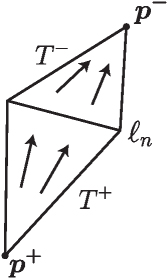
Figure 3: RWG function on a pair of adjacent triangles.

2. Half-RWG

The half-RWG basis function is a modified version of its original counterpart and is defined only in a single triangle of mesh $ℳ$ [61], as shown in Fig. 4. Every edge ${\mathrm{\ell }}_n\in ℳ$ has an arbitrarily generated direction. However, this direction is fixed, so the edge vector ${\mathbf{\ell }}_n$ of each edge is constant. Also, the reference normal unit vector ${\widehat{\mathbf{n}}}^{ref}$ points towards the direction that is the result of the counterclockwise rotation of the triangle’s vertices (their order is initially defined once for each triangle). The half-RWG function associated with an edge ${\mathrm{\ell }}_n$ of a mesh triangle $T$ with area $A$ is defined as

${\mathbf{h}}_n\left(\mathbf{r}\right)=\{\begin{array}{ccc}{\displaystyle \frac{\pm {\mathrm{\ell }}_n}{2A}}\left(\mathbf{r}-\mathbf{p}\right),\hfill & \mathbf{r}\in T\hfill & \\ 0,\hfill & \mathrm{otherwise}\hfill & \end{array},$

(78)

where $\mathbf{p}$ is the vertex of $T$ across ${\mathrm{\ell }}_n$. The sign of ${\mathbf{h}}_n\left(\mathbf{r}\right)$ in each of the problem’s domains ${\mathrm{\Omega }}_i$ is different for opposite sides of the boundary between two adjacent domains. Hence, if ${\mathrm{\Omega }}_{\mathrm{\ell }}$ and ${\mathrm{\Omega }}_m$ have a common boundary, then ${\mathbf{h}}_{n,\mathrm{\ell }}\left(\mathbf{r}\right)=-{\mathbf{h}}_{n,m}\left(\mathbf{r}\right)$. This means that the boundary conditions regarding the surface electric and magnetic current densities are satisfied by half-RWG, when using the same expansion coefficients. As a result, some signs in the formulations that were previously presented will change with the use of this function. By employing the continuity of the original RWG-functions, the cumulative RWG function is defined as

$${\mathbf{f}}_n\left(\mathbf{r}\right)=\sum _{\{k:{\mathrm{\ell }}_k={\mathrm{\ell }}_n\}}{\mathbf{h}}_k\left(\mathbf{r}\right),$$

(79)

where ${\mathbf{f}}_n\left(\mathbf{r}\right)$ refers to an edge ${\mathrm{\ell }}_n$ and ${\mathbf{h}}_k\left(\mathbf{r}\right)$ refers to a half-RWG basis function that borders ${\mathrm{\ell }}_n$.

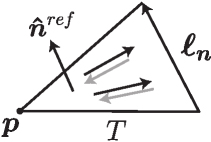
Figure 4: Half-RWG function defined on a single mesh triangle.

3. Buffa-Christiansen (BC)

Another divergence-conforming and quasi-curl-conforming basis function is the BC function, which is defined on a barycentric refinement ${ℳ}_b$ of the original triangular mesh $ℳ$ [62]. Essentially, it is a linear combination of a set of RWG functions which are defined on ${ℳ}_b$. However, a BC function is associated with an edge of the original mesh $ℳ$.

Consider a reference edge ${\mathrm{\ell }}_n$ on the original mesh $ℳ$. The barycentric refinement ${ℳ}_b$ is presented in Fig. 5.

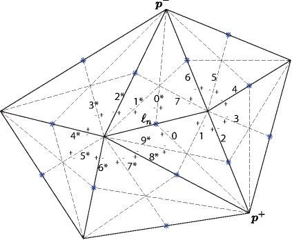
Figure 5: Barycentically refined mesh ${ℳ}_b$.

Around the right and left vertices of the reference edge there are $N_c=4$ and $N_c^{\ast }=5$ triangles, respectively, that belong to $ℳ$. In Fig. 5 the plus ($+$) and minus ($-$) signs show the appropriate direction of the numbered RWG functions (or half-RWG for open surfaces) on the new edges of ${ℳ}_b$. The linear combination of these functions, with appropriate signs and coefficients, synthesizes the BC basis function of the reference edge. The aforementioned coefficients are defined as follows [51],

$c_i$

$=\{\begin{array}{ccc}{\displaystyle \frac{1}{2l_0}},\hfill & i=0\hfill & \\ {\displaystyle \frac{N_c-i}{2l_i{N}_c}},\hfill & i=1,\mathrm{\dots },2N_c-1\hfill & \end{array},$

(80)

$c_{i^{\ast }}$

$=\{\begin{array}{ccc}-{\displaystyle \frac{1}{2l_{0^{\ast }}}},\hfill & i^{\ast }=0\hfill & \\ -{\displaystyle \frac{N_c^{\ast }-i^{\ast }}{2l_{i^{\ast }}{N}_c^{\ast }}},\hfill & i^{\ast }=1^{\ast },\mathrm{\dots },2N_c^{\ast }-1.\hfill & \end{array}$

(81)

The form of the BC for the reference edge ${\mathrm{\ell }}_n$ is shown in Fig. 6.

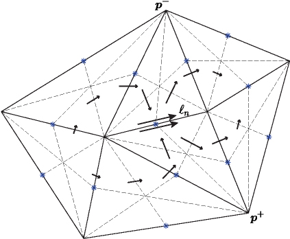
Figure 6: Buffa-Christiansen basis function.

The BC functions present however a significant drawback regarding the representation of the surface charge density since they model the surface charge density as a constant function around the vertices of the original mesh $ℳ$ [42]. The RWG functions present constant surface charge density inside the triangular elements, as mentioned in the previous section. Hence, the latter are more appropriate for modeling discontinuous and singular surface charge density near sharp corners [63].

${\mathbf{f}}_n^{LL,1}\left(\mathbf{r}\right)$

$=\{\begin{array}{ccc}{\displaystyle \frac{{\mathrm{\ell }}_n}{4{\left(A^{+}\right)}^2}}\left(\mathbf{r}-{\mathbf{r}}_1\right)\cdot \left[\left({\mathbf{r}}_4-{\mathbf{r}}_1\right)\times \widehat{\mathbf{n}}\left(\mathbf{r}\right)\right]\left({\mathbf{r}}_3-{\mathbf{r}}_1\right),\hfill & \mathbf{r}\in T^{+}\hfill & \\ {\displaystyle \frac{{\mathrm{\ell }}_n}{4{\left(A^{-}\right)}^2}}\left(\mathbf{r}-{\mathbf{r}}_2\right)\cdot \left[\left({\mathbf{r}}_4-{\mathbf{r}}_2\right)\times \widehat{\mathbf{n}}\left(\mathbf{r}\right)\right]\left({\mathbf{r}}_3-{\mathbf{r}}_2\right),\hfill & \mathbf{r}\in T^{-}\hfill & \\ 0,\hfill & \mathrm{otherwise}\hfill & \end{array}$

(82)

${\mathbf{f}}_n^{LL,2}\left(\mathbf{r}\right)$

$=\{\begin{array}{ccc}{\displaystyle \frac{{\mathrm{\ell }}_n}{4{\left(A^{+}\right)}^2}}\left({\mathbf{r}}_1-\mathbf{r}\right)\cdot \left[\left({\mathbf{r}}_3-{\mathbf{r}}_1\right)\times \widehat{\mathbf{n}}\left(\mathbf{r}\right)\right]\left({\mathbf{r}}_4-{\mathbf{r}}_1\right),\hfill & \mathbf{r}\in T^{+}\hfill & \\ {\displaystyle \frac{{\mathrm{\ell }}_n}{4{\left(A^{-}\right)}^2}}\left({\mathbf{r}}_2-\mathbf{r}\right)\cdot \left[\left({\mathbf{r}}_3-{\mathbf{r}}_2\right)\times \widehat{\mathbf{n}}\left(\mathbf{r}\right)\right]\left({\mathbf{r}}_4-{\mathbf{r}}_2\right),\hfill & \mathbf{r}\in T^{-}\hfill & \\ 0,\hfill & \mathrm{otherwise}\hfill & \end{array}$

(83)

4. Trintinalia-Ling (TL)

The TL basis function [64], also called linear-linear (LL) basis function [65], can be perceived as a decomposition of the RWG basis function. Indeed, consider a triangular mesh $ℳ$ on a surface; the first and the second kind of LL functions are defined for every pair of adjacent triangles $T^{+}$ and $T^{-}$ with a common edge ${\mathrm{\ell }}_n$, as shown below. Figures 7 and 8 show the form of both kinds of LL basis functions.

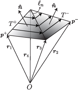
Figure 7: First kind of LL basis function.

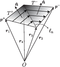
Figure 8: Second kind of LL basis function.

The grayscale gradient inside the triangles illustrates the magnitude of the basis function. The analytical formulas of the first and second kinds of LL basis functions are given by (82) and (83), where ${\mathrm{\ell }}_n$ is the length of the common edge and $A^{+}$ and $A^{-}$ are the areas of $T^{+}$ and $T^{-}$.

For both kinds of LL functions, the spatial distribution is parallel to the surrounding edges where the magnitude of the basis function is nonzero (non-white color in Figs. 7 and 8). Also, it varies linearly along those edges (maximum at the intersection with the reference edge ${\mathrm{\ell }}_n$). What is more, it is zero next to the surrounding edges where the magnitude of the basis function is zero (white color). Lastly, it exhibits a linear variation on the reference edge ${\mathrm{\ell }}_n$ for both perpendicular and tangential directions.

As mentioned previously, a testing procedure with a function is required to convert the surface integral equation into a matrix equation. In this sense, the proper testing functions have to be selected for the MoM implementation, such that the final system leads to accurate solutions. In order to understand this, the mapping properties of surface integral operators have to be examined. Consider the following finite element spaces:

	${ℛ}_{ℳ}$	$={\left\{{\mathrm{RWG}}_j\right\}}_{j=1}^{N_e},$		(86)
	${ℛ}_{ℳ}^n$	$={\left\{\widehat{\mathbf{n}}\times {\mathrm{RWG}}_j\right\}}_{j=1}^{N_e},$		(87)
	${ℬ}_{ℳ}$	$={\left\{{\mathrm{BC}}_j\right\}}_{j=1}^{N_e},$		(88)
	${ℬ}_{ℳ}^n$	$={\left\{\widehat{\mathbf{n}}\times {\mathrm{BC}}_j\right\}}_{j=1}^{N_e},$		(89)

where $ℳ$ is the original mesh and $N_e$ is the number of edges in $ℳ$. Regarding the previously presented formulations, the mapping properties of the discretized integral operators for RWG functions are [34]

	${𝒟}^n$	$:{ℛ}_{ℳ}⟶{ℬ}_{ℳ},$		(90)
	${𝒟}^t$	$:{ℛ}_{ℳ}⟶{ℬ}_{ℳ}^n,$		(91)
	$\left({𝒦}^n\pm {\displaystyle \frac{ℐ}{2}}\right)$	$:{ℛ}_{ℳ}⟶{ℛ}_{ℳ},$		(92)
	$\left({𝒦}^t\pm {\displaystyle \frac{{ℐ}_n}{2}}\right)$	$:{ℛ}_{ℳ}⟶{ℛ}_{ℳ}^n.$		(93)

As far as BC functions are concerned, the analogous mapping properties are the following [66]

	${𝒟}^n$	$:{ℬ}_{ℳ}⟶{ℛ}_{ℳ},$		(94)
	${𝒟}^t$	$:{ℬ}_{ℳ}⟶{ℛ}_{ℳ}^n,$		(95)
	$\left({𝒦}^n\pm {\displaystyle \frac{ℐ}{2}}\right)$	$:{ℬ}_{ℳ}⟶{ℬ}_{ℳ},$		(96)
	$\left({𝒦}^t\pm {\displaystyle \frac{{ℐ}_n}{2}}\right)$	$:{ℬ}_{ℳ}⟶{ℬ}_{ℳ}^n.$		(97)

Regarding the above spaces, the $\widehat{\mathbf{n}}\times \mathrm{RWG}$ function space is not an $L^2$ dual of the RWG space, but the $\widehat{\mathbf{n}}\times \mathrm{BC}$ function space is [34]. The same goes for the $\widehat{\mathbf{n}}\times \mathrm{RWG}$ and BC function spaces. In each formulation, the integral operators that provide the main contributions to the final matrix system (elements around the diagonal) have to be well tested. It has been shown that testing the surface integral operators with the dual of their range space leads to the most accurate results [66]. Thus, the basis function that is used to expand the main contributing integral operators will determine the choice of the testing function, as will be presented in section V.B..

D. Singularity subtraction

The use of SIEs with the MoM produces singular integrals with weakly- or hyper-singular surface integral operators. These singularities appear when the basis and testing functions belong to the same triangular element or to adjacent triangles that share an edge or a vertex. The reason for these singularities is the denominator of Green’s function, that goes to zero as $R=\left|\mathbf{r}-{\mathbf{r}}^{\prime }\right|=0$, when $\mathbf{r}={\mathbf{r}}^{\prime }$. The solution to this problem can be given by the application of a singularity subtraction method [67].

In order to implement the method, the Green’s function in a domain ${\mathrm{\Omega }}_i$ has to be expanded in a Taylor series, as follows,

$$G_i(\mathbf{r},{\mathbf{r}}^{\prime })=\frac{1}{4\pi }\left(\frac{1}{R}+j{k}_i-\frac{k_i^{2}R}{2}+\frac{j{k}_i^2{R}^2}{6}-\mathrm{\dots }\right),$$

(98)

where the odd terms are the singular ones ($q=-1,1,3,\mathrm{\dots }$). In this sense, Green’s function can be divided into a free of singularities smooth part and a singular part, hence

$$G_i(\mathbf{r},{\mathbf{r}}^{\prime })=G_i^s(\mathbf{r},{\mathbf{r}}^{\prime })+T_i(\mathbf{r},{\mathbf{r}}^{\prime }),$$

(99)

where

	$G_i^s(\mathbf{r},{\mathbf{r}}^{\prime })$	$={\displaystyle \frac{e^{j{k}_{i}R}}{4\pi R}}-{\displaystyle \frac{1}{4\pi R}}+{\displaystyle \frac{k_i^{2}R}{8\pi }},$		(100)
	$T_i(\mathbf{r},{\mathbf{r}}^{\prime })$	$={\displaystyle \frac{1}{4\pi R}}-{\displaystyle \frac{k_i^{2}R}{8\pi }}.$		(101)

Thus, the smooth part $G_i^s(\mathbf{r},{\mathbf{r}}^{\prime })$ can be accurately integrated numerically and the singular part $T_i(\mathbf{r},{\mathbf{r}}^{\prime })$ can be integrated semi-analytically with the help of closed-form relations. In Fig. 9 we present the normalized values of the real part of the scalar Green’s function, the real part of the smoothed term $G_i^s(\mathbf{r},{\mathbf{r}}^{\prime })$ and the singular term $T_i(\mathbf{r},{\mathbf{r}}^{\prime })$ as a function of the electrical distance $k_{i}R$. The subtraction of the first odd term would be enough for making the smooth part non-singular, but in this case Green’s function would have a discontinuous derivative at $R=0$. Also, the term $k_{i}R$ is small for the case of singularities so the first and the second odd terms are enough for the definition of $G_i^s(\mathbf{r},{\mathbf{r}}^{\prime })$, since odd terms of higher orders diminish rapidly for small values of $k_{i}R$ [68].

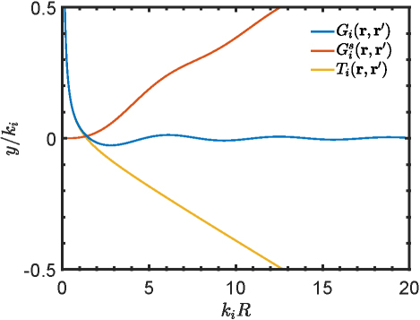
Figure 9: Graphical representation of singularity subtraction.

The integrals that occur from the implementation of the singularity subtraction method are the following

	$I_1^q$	$={\displaystyle {\int }_{\partial {\mathrm{\Omega }}_i}}dS\left[\nabla \cdot {\mathbf{f}}_m\left(\mathbf{r}\right)\right]{\displaystyle {\int }_{\partial {\mathrm{\Omega }}_i}}d{S}^{\prime }{R}^q{\nabla }^{\prime }\cdot {\mathbf{f}}_n\left({\mathbf{r}}^{\prime }\right),$		(102)
	$I_2^q$	$={\displaystyle {\int }_{\partial {\mathrm{\Omega }}_i}}dS{\mathbf{f}}_m\left(\mathbf{r}\right)\cdot {\displaystyle {\int }_{\partial {\mathrm{\Omega }}_i}}d{S}^{\prime }{R}^q{\mathbf{f}}_n\left({\mathbf{r}}^{\prime }\right),$		(103)
	$I_3^q$	$={\displaystyle {\int }_{\partial {\mathrm{\Omega }}_i}}dS{\mathbf{f}}_m\left(\mathbf{r}\right)\cdot {\displaystyle {\int }_{\partial {\mathrm{\Omega }}_i}}d{S}^{\prime }\left({\nabla }^{\prime }{R}^q\right)\times {\mathbf{f}}_n\left({\mathbf{r}}^{\prime }\right),$		(104)

where ${\mathbf{f}}_m\left(\mathbf{r}\right)$ is the testing function, ${\mathbf{f}}_n\left(\mathbf{r}\right)$ is the basis function and $q=-1,1$. The aforementioned integrals are solved semi-analytically, which means that the inner integrals are solved analytically for arbitrary $\mathbf{r}$, with closed-form expressions, and the outer integrals are solved numerically. The closed-form relations for the inner integrals can be found in [68].

V. FORMULATION AND DISCRETIZATION COMPARISONS

The previous considerations highlight the need to discuss in the following sections many different aspects of SIE methods, including the comparison between different formulations, as well as different basis and testing functions.

A. Comparison of different formulations

Table 1: Comparison of different formulations

Set of Formulations	Test Function	Basis Function	Reference
T-PMCHWT, CTF, ICTF	RWG	RWG	[69]
T-PMCHWT, mN-Müller, JMCFIE, NFM, DDA	RWG	RWG	[70]
T-PMCHWT, N-Müller, CTF, CNF, JMCFIE	RWG	RWG	[71]
T-PMCHWT, CTF, CNF, N-Müller, mN-Müller, JMCFIE	RWG	RWG	[48]
T-PMCHWT, CTF, CNF, N-Müller, mN-Müller, JMCFIE	TL	TL	[48]
T-PMCHWT, N-Müller, T-Müller	RWG	RWG	[47]
T-PMCHWT, CTF, CNF, N-Müller, T-PMCHWT (CMP)	RWG	RWG	[72]

In this section, we compare the different SIE formulations – namely mN-Müller, T-PMCHWT and JMCFIE – for the case of a spherical gold nanostructure with a radius $r=100$ nm in an air background, which presents the advantage that the analytical Mie solution can be considered as reference. A detailed discussion of the results for this case, as well as for some more general shape scatterers, can be found in [70]. We assume that the incident plane wave is propagating along the $z$-axis and has linear polarization towards the $x$-axis. The wavelength is $\lambda =550$ nm (monochromatic results, such as the bistatic scattering cross section in Fig. 10) and the following figures were obtained with RWG basis functions and the Galerkin method.

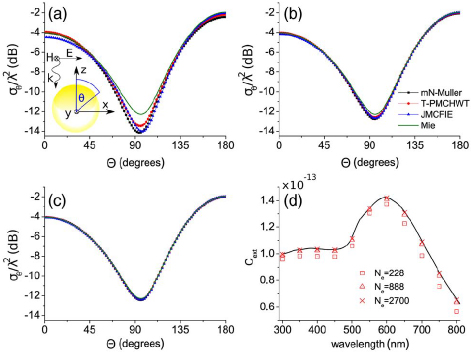
Figure 10: Bistatic scattering cross section of a gold sphere ($r=100$ nm) for three mesh densities with (a) $N_e=228$, (b) $N_e=888$, (c) $N_e=2700$ number of edges and (d) extinction $C_{ext}$ spectrum obtained by the T-PMCHWT for the three meshes compared to the Mie solution. Adapted with permission from [70] $\mathrm{\copyright }$ Optica Publishing Group.

It is expected that, as the number of unknowns increases, the different formulations tend to approximate better the Mie solution. However, T-PMCHWT seems to be closer to the Mie solution than other formulations for a smaller number of unknowns, see Fig. 10 (a). The very good matching of this formulation with the analytical solution is explained in Fig. 10 (d), where the spectrum of the sphere’s extinction cross section $C_{ext}$, which is extracted via T-PMCHWT, is compared to the Mie theory solution.

As shown in Fig. 11 (b), all three formulations present the same level of accuracy in the near-field zone, where the tangential component of the scattered electric field intensity (on the sphere) is considered for the error extraction. However, in the far-zone, where $C_{ext}$ is taken into account for error calculations, JMCFIE performs the best, followed by T-PMCHWT. The mN-Müller presents the highest error of the three, see Fig. 11 (a). In [73] the strong material dependencies of conventional formulations, such as the normal and scaled forms of T-PMCHWT, CTF, JMCFIE and others, are examined and their performances for different plasmonic nanostructure problems are presented. In Table 1 we present some of the papers that examine and compare different formulations of the SIE method, including some that were not discussed before; the combined tangential formulation (CTF), the improved combined tangential formulation (ICTF), the null field method (NFM) and the combined normal formulation (CNF), while CMP in the last row of Table 1 stands for Calderon multiplicative preconditioner [51, 52].

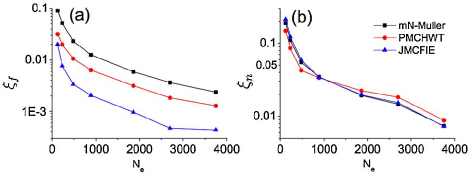
Figure 11: Error in (a) the far zone ${\xi }_f$ and (b) the near zone ${\xi }_n$ of a gold sphere ($r=100$ nm) obtained with the mN-Müller, T-PMCHWT, and JMCFIE formulations as a function of the number of mesh edges $N_e$. Adapted with permission from [70] $\mathrm{\copyright }$ Optica Publishing Group.

B. Basis and testing functions comparisons

As mentioned in section IV.C., the use of the dual of the range of integral operators for testing leads to more accurate results. For the integral equations of the first kind, like EFIE and T-PMCHWT, this is identical with Galerkin’s method, but for the integral equations of the second kind, like MFIE and mN-Müller, this leads the use of the Petrov–Galerkin method with appropriate curl-conforming testing functions. Moreover, the use of hybrid meshes introduces additional complexity and intriguing capabilities, while it also affects the condition number of the final system and the total simulation time, as shown in [74]. In [66] there is a very detailed examination of many different formulations, discretization schemes and problems, but we will focus mostly on the cases of T-PMCHWT andN-Müller.

In Fig. 12, the fact that the dual of the range of integral operators is better for testing in terms of accuracy is confirmed, while Table 2 presents all the different cases of dual testing for the T-PMCHWT formulation. Figure 12 shows that, for the T-PMCHWT formulation, when both RWG and BC are used as basis functions in a mixed discretization scheme (i.e. the cases Dual (RB) and Dual (BR) in the last two rows of Table 2), the results are worse than the Galerkin method with RWG functions as both testing and basis functions.

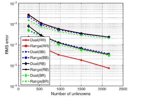
Figure 12: RMS error of the bistatic RCS in the E-plane computed with the T-PMCHWT formulation. Dielectric sphere with $k_{0}a=1$ and ${\epsilon }_r=4$, ${\mu }_r=1$. Adapted with permission from [66] $\mathrm{\copyright }$ John Wiley & Sons.

Table 2: T-PMCHWT test & basis function pairs

Method	$\mathbf{J}$	$\mathbf{M}$	EFIE	MFIE
Dual (RR)	RWG	RWG	RWG	RWG
Dual (BB)	BC	BC	BC	BC
Dual (RB)	RWG	BC	RWG	BC
Dual (BR)	BC	RWG	BC	RWG

Table 3: mN-Müller test & basis function pairs

Method	$\mathbf{J}$	$\mathbf{M}$	MFIE	EFIE
Dual (RR)	RWG	RWG	n$\times$BC	n$\times$BC
Dual (BB)	BC	BC	n$\times$RWG	n$\times$RWG
Dual (RB)	RWG	BC	n$\times$BC	n$\times$RWG
Dual (BR)	BC	RWG	n$\times$RWG	n$\times$BC

Table 4: Comparison of different discretization schemes

Formulations	Test & Basis Functions Pairs	References
MFIE	(RWG, RWG) and ($\widehat{\mathbf{n}}\times$RWG, $\widehat{\mathbf{n}}\times$RWG)	[75]
MFIE	(RWG, RWG), ($\widehat{\mathbf{n}}\times$RWG, $\widehat{\mathbf{n}}\times$RWG), and	[76, 77]
	(monopolar RWG, monopolar RWG)
MFIE	(LL, LL) and (RWG, RWG)	[65, 78]
PMCHWT	($\widehat{\mathbf{n}}\times$RWG, RWG)	[41]
Müller	(RWG, RWG) and ($\widehat{\mathbf{n}}\times$BC, RWG)	[41]
N-Müller	(RWG, RWG) and ($\widehat{\mathbf{n}}\times$BC, RWG)	[32]
EFIE	(RWG, RWG) and (BC, BC)	[66]
MFIE	($\widehat{\mathbf{n}}\times$BC, RWG) and ($\widehat{\mathbf{n}}\times$RWG, BC)	[66]
PMCHWT	(RWG, RWG), (BC, BC), (Mixed RWG-BC, Mixed RWG-BC), and	[66]
	(Mixed BC-RWG, Mixed BC-RWG)
mN-Müller	($\widehat{\mathbf{n}}\times$BC, RWG), (Mixed $\widehat{\mathbf{n}}\times$BC-$\widehat{\mathbf{n}}\times$RWG, Mixed RWG-BC),	[66]
	($\widehat{\mathbf{n}}\times$RWG, BC), and (Mixed $\widehat{\mathbf{n}}\times$RWG-$\widehat{\mathbf{n}}\times$BC, Mixed BC-RWG)
MFIE, CFIE	Higher order test & basis functions	[79]
mN-Müller, JMCFIE	Higher order test & basis functions	[79]

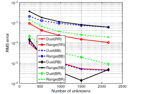
Figure 13: RMS error of the bistatic RCS in the E-plane computed with the mN-Müller formulation. Dielectric sphere with $k_{0}a=1$ and ${\epsilon }_r=4$, ${\mu }_r=1$. Adapted with permission from [66] $\mathrm{\copyright }$ John Wiley & Sons.

For the mN-Müller formulation, the reference Table 3 presents all the different cases of dual testing. Figure 13 presents similar results, but for the case of a mN-Müller formulation. In the case of the sphere, which is a smooth object, the mN-Müller gives a more accurate solution, compared to the results of the T-PMCHWT formulation, when the Dual(RB) mixed discretization scheme is used. However, for objects that are not smooth, such as cubes and prisms, the T-PMCHWT formulation is more accurate than the mN-Müller formulation. Lastly, a comprehensive comparison of different discretization schemes, including the various test and basis function pairings used in common formulations, is presented in Table 4.

VI. NUMERICAL SOLVERS AND APPROACHES

As mentioned in previous sections, integral equations are converted into the final linear system with the aid of a set of testing and basis functions. However, a significant challenge in SIE methods has been the appearance of large dense matrices after the discretization of complex real-life electromagnetic scattering problems. In the 1980s, the capabilities of MoM solvers were illustrated in [80], which highlighted that the largest problem solvable via direct lower–upper (LU) factorization within an hour was still relatively modest in size. The general consensus at the time was that MoM would not be a viable approach for real-world scattering scenarios due to its high computational cost and limited scalability, since it scaled as $𝒪(N^2)$ in terms of memory consumption while having a complexity of $𝒪(N^3)$ for direct solvers. In terms of iterative solvers, the dense matrix equations involving $𝒪(N)$ unknowns can be addressed via a Krylov-subspace algorithm, such as the generalized minimum residual (GMRES), conjugate gradient (CG), and bi-conjugate stabilized (BiCGStab) [81], but the aforementioned bottlenecks make their application to large-scale models impractical. Another key challenge of the SIE method is that some formulations (e.g. the EFIE and PMCHWT) belong to the first kind of integral equations. As a result, the final linear systems tend to be ill-conditioned, prompting the need for additional techniques, such as regularization or specialized preconditioning, to ensure that the resulting matrices are well-conditioned and can be solved efficiently. Also,an ill-conditioned final matrix system can occur when SIEs are used for low frequency simulations. However, the advancement of the Calderon preconditioner, along with the development of various numerical approaches for both direct [82] and iterative solvers [83, 84], and particularly the implementation of fast solvers, have helped mitigate these difficulties.

A. Low frequency breakdown

When the SIE method is used for electrically small yet complex geometries or with very dense discretizations, a recurring challenge known as the low frequency breakdown problem arises. This issue has been extensively analyzed in [85, 86]. One common strategy for handling the low‐frequency regime, while preserving the correct physical behavior, is to employ loop‐tree or loop‐star basis functions combined with a suitable frequency normalization approach. Nevertheless, fast methods like the multi-level fast multipole algorithm (MLFMA) typically fail when the frequency is very low [87].

Even with loop‐tree or loop‐star basis functions, iterative solvers may still experience high iteration counts. The root cause is linked to the divergence properties of the RWG basis, which are not ideal for accurately representing charges at low frequencies [88]. To address this, a basis‐rearrangement scheme was introduced in [88, 89]. Reshaping the way the basis functions are assembled substantially enhances the eigenvalue spectrum of the final system matrix and reduces notably the iteration count.

B. Calderon preconditioner

Calderon preconditioning is a regularization technique for SIEs [90, 40, 51, 52]. This approach utilizes the self-regularization property of the electric-field integral operator (EFIO), commonly referred to as the Calderon integral identity [56], which can be written as:

$${\left({𝒟}^n\right)}^2=-\frac{1}{4}ℐ+{\left({𝒦}^n\right)}^2,$$

(105)

where the notation of the previous sections is followed for the integral operators. The subscript $i$ is missing, since for the final system to be formed, a summation over all domains has been executed. This identity demonstrates that when the EFIO (${𝒟}^n$) is multiplied by itself, the resulting operator is better conditioned, particularly on sufficiently smooth surfaces where it approximates the summation of a compact and an identity operator. When the CMP (which was called Calderon multiplicative preconditioner in previous sections) is applied with the RWG and Buffa-Christiansen functions, it not only mitigates the ill-conditioning of the EFIO, but also maintains the solution accuracy [51].

Mathematically, the operator ${\left({𝒟}^n\right)}^2$ establishes the mapping:

$${\left({𝒟}^n\right)}^2:H^{-1/2}(\mathrm{div},\partial \mathrm{\Omega })\to H^{-1/2}(\mathrm{div},\partial \mathrm{\Omega }),$$

(106)

hence the application of the Calderon multiplicative preconditioner on the EFIE (CMP-EFIE) leads to a range space that is identical with that of the MFIE. This equivalence allows them to be effectively combined into a CFIE, which is inherently better conditioned than its non-preconditioned counterpart. However, the resulting CFIE system is not a resonance-free formulation, as the CMP-EFIE and the MFIE share the same resonances [91]. Lastly, Calderon preconditioning has also been extended for the PMCHWT formulation in the case of homogeneous isotropic [92] and chiral objects [93].

C. Iterative fast solvers

Iterative solutions require matrix-vector multiplications (MVMs), thus the development of a fast algorithm to solve the MoM equation requires the combination of an iterative method with a fast approach to compute the MVMs. Over the last few decades, a variety of fast solvers have been developed to overcome the high computational and memory costs traditionally associated with the MoM solution of SIEs. In general, fast algorithms broadly fall into two categories: kernel‐dependent, which are influenced by the specific properties of the underlying Green’s function, and kernel‐independent, which leverage low‐rank representations of system sub‐blocks without requiring explicit knowledge of the integral operator’s closed‐form expansions.

One of the most impactful kernel‐dependent solvers is the multilevel fast multipole method (MLFMM) [94, 4], which is an extension of the fast multipole method (FMM) [95, 96]. As presented in [97], in order to implement the MLFMM, the entire scatterer is initially enclosed within a large auxiliary cubic box, which is then divided into eight smaller cubes. This domain subdivision process continues recursively until the smallest cubes have an edge length that is comparable to the wavelength ($\approx \lambda /2$). Each cube at every level of this process is assigned an index. At the finest level, the cube containing each basis function is identified by comparing the coordinates of the basis function’s center with the cube’s center. Additionally, nonempty cubes are identified through a sorting process, and only these cubes are stored using a tree-structured data format [97]. Hence, the method organizes the interactions of basis-testing functions into a tree structure with multiple levels of hierarchically defined groups (clustering) of varying fineness, by utilizing the analytical expansion of Green’s function and addition theorem [98]. Short-range (near-field) interactions are calculated directly and stored in memory, while long-range (far‐field) interactions are performed efficiently using the factorization/diagonalization of the Green’s function, thus reducing both the memory requirement and computational time complexity (MVM speed) to approximately $𝒪(N\log N)$ for 3D electromagnetic scattering problems [98]. The introduction of this method marked a significant shift in computational electromagnetics, allowing MoM to tackle very large problems in terms of electrical size, while retaining its accuracy. The approach is widely parallelized in practice [99, 100, 101], making it one of the leading techniques for real‐world large‐scale modeling.

Another group of kernel‐dependent solvers consists of the grid- or fast Fourier transform (FFT)‐based techniques. The latter leverage the translation invariance of the kernel function, which can reduce the memory requirement and central processing unit (CPU) time complexity of 3D problems. Two of the most popular methods of this group are the pre‐corrected FFT (p‐FFT) and adaptive integral method (AIM), which typically achieve $𝒪(N^{1.5})$ for storage and $𝒪(N^{1.5}\log N)$ for MVM. More specifically, both methods rely on an equivalent source approximation. As described in [102], the acceleration of computations with the application of FFT requires the entire scatterer to be enclosed within an auxiliary rectangular domain. Afterwards, this auxiliary domain is recursively divided into a uniform Cartesian grid, ensuring that each small cube contains at most a few discretization elements. To perform the MVM with FFT, the original basis functions are mapped onto the Cartesian grid, which is achieved through basis transformation. Additionally, a fast high-order algorithm for solving surface scattering problems, utilizing a two-face equivalent source approximation, is presented in [103]. This method achieves computational complexities ranging from $𝒪(N^{6/5}\log N)$ to $𝒪(N^{4/3}\log N)$, by strategically positioning equivalent sources solely on the faces of cubic cells. In [104], the Sparse‐Matrix/Canonical‐Grid (SM/CG) technique is presented. Unlike the previously discussed approaches, it does not make use of equivalent sources; instead, it applies a Taylor series expansion of the Green’s function on a regularly spaced canonical grid. The system matrix is then handled via an FFT‐driven iterative scheme, where the number of Taylor expansion terms dictates the procedure. However, the SM/CG method demands detailed knowledge of the integral kernel, while its memory complexity scales as $𝒪(N^{1.5})$. In [105], the Quadrature Sampled Pre‐Corrected Fast‐Fourier Transform (QS‐PCFFT) method was introduced. This approach projects the unknown currents onto a uniform grid and computes the discrete Fourier transform of the current directly by means of a discontinuous FFT, employing quadrature sampling for the currents. As a result, it achieves adjustable accuracy and exponential convergence. Furthermore, the Green’s function interpolation combined with the FFT algorithm (GIFFT) [106] was developed to handle arrays of arbitrary shape. In GIFFT, an array mask function identifies array boundaries and determines where the Green’s function should be interpolated. The MVMs in the iterative solver are then accelerated via FFT, reducing both storage requirements and overall solution time. Nonetheless, for SIEs, none of the aforementioned FFT‐based techniques achieves asymptotically better performance than MLFMM. Finally, most iterative methods are sensitive to the condition number of matrix systems, and the number of iterations needed to reach the desired accuracy varies depending on the problem. Even though preconditioning techniques and domain decomposition methods have been developed to address many of these challenges, convergence remains not entirely predictable.

D. Direct fast solvers

In parallel, direct fast solvers utilizing hierarchical matrices (H-matrices) and matrix compression techniques have introduced kernel-independent algebraic methods. The latter rely on the observation that well‐separated sub‐blocks of the dense system matrix exhibit numerical rank deficiency. Algorithms such as the adaptive cross approximation (ACA) [107] compress these sub‐blocks without requiring explicit expansions of the integral kernel.

The research of fast direct solvers for SIEs seek to address the drawbacks highlighted earlier. There are a number of fundamental studies that have laid the groundwork for direct solution techniques [108, 109, 110, 111], many of which have since influenced advances in computational electromagnetics.

As presented in [82], early investigations include the ${\text{IES}}^3$ algorithm [112], direct treatments for 2D slender scatterers [113], and a compressed block decomposition (CBD) algorithm for capacitance extraction that combines matrix decomposition with singular value decomposition (SVD) [114]. Furthermore, an application of a multilevel nonuniform grid (MLNG) approach for direct inversion of the EFIE was presented some years ago in [115].

Meanwhile, the concept of H‐matrices [116, 117], which systematically apply low‐rank compression to well‐separated matrix subgroups, has become a recognized framework for hierarchical direct solvers. Since this approach relies on certain smoothness criteria for the integral kernel, it typically applies to mid‐ and low‐frequency regimes in electromagnetics, where the oscillatory nature of the kernel is less pronounced [118]. However, numerous implementations have adopted various H-matrix techniques [119, 120, 121]. Additional comparisons between multilevel block inversion and multilevel LU decomposition have also been made [122]. Another line of research incorporates the butterfly algorithm with randomized compression, achieving $𝒪(N{\log }^{2}N)$ scaling and supporting large‐scale 3D SIE simulations for PEC [123]. For penetrable scatterers, a quasi‐block‐Cholesky (QBC) approach that investigates the checkerboard symmetry pattern in the PMCHWT system matrix was proposed in [124], while a butterfly‐based multilevel matrix decomposition algorithm (MLMDA) for homogeneous penetrable objects was presented in [125]. Finally, in [82] a more detailed discussion on works that are based on the following matrix structures is provided: hierarchical off‐diagonal low‐rank (HODLR), hierarchically semiseparable (HSS), and ${\text{H}}^2$ matrices.

E. Higher order methods

Another development in integral equation methods has been the use of higher order isoparametric elements [126, 127]. Recently, it was shown that hybrid discretization schemes can affect the condition number of the final matrix system and the efficiency of the solution procedure [74]. This insight further reinforces the idea of using higher order techniques to improve the numerical behavior of SIEs. In many electromagnetic radiation and scattering problems, the primary source of numerical error often arises from inaccuracies in geometric modeling [87]. The use of these elements not only mitigates the aforementioned error, but also enables exponential error convergence in regions where the numerical solutions remain smooth [87].

There are two main approaches to employ higher order isoparametric elements in solving SIEs, namely the Galerkin [126, 127] and Nystrom methods [92, 105]. Both approaches have demonstrated higher order convergence rates for electromagnetic problems characterized by smooth solutions. A very detailed and comprehensive review of the higher order computational electromagnetics for antenna, wireless, and microwave engineering applications is presented in [128].

F. Parallelization and high-performance computing

High‐performance computing (HPC) resources have been widely and effectively employed by researchers and engineers in the area of computational electromagnetics. Over time, developments in computing hardware and software have created extraordinary possibilities (and new challenges) for expanding the modeling techniques used for scattering problems. Crucially, these advances have taken place in parallel with progress in electromagnetic formulations and numerical algorithms. The research community has been especially resourceful in capitalizing on every available advance in hardware and technology.

Traditionally, two primary parallel programming paradigms, open multiprocessing (OpenMP) and the message passing interface (MPI), have dominated the landscape. These frameworks can facilitate massively parallel MLFMM simulations involving billions of unknowns [129, 100].

A historical perspective highlights the scale of these achievements. In 1988, Miller illustrated how the largest feasible problem within a one‐hour time frame advanced from only around 100 unknowns in the early 1950s to approximately 6,000 unknowns (roughly a factor of 60) by the mid‐1980s [80]. However, over the next few decades, this capability surged to approximately 10.5 billion unknowns within about 6.25 hours [100], yielding an increase on the order of 1.75 million. Thus, while the first half‐century of computational electromagnetics and SIEs may have appeared to progress relatively slowly, the subsequent 30 years saw an explosive expansion of modeling capacity. Additionally, graphics processing units (GPUs), which were originally designed for computer graphics, evolved into indispensable hardware accelerators that can be used with the SIE method. As shown in Table 5, the utilization of GPUs can significantly enhance the efficiency of the SIE method [99]. More specifically, Table 5 includes time data regarding the calculation of radiation patterns of the basis functions ${\mathbf{V}}_s$, receiving patterns of the testing functions ${\mathbf{V}}_f$, the translator factor $\mathbf{T}$, and the assembly of the near-field system matrix ${\mathbf{Z}}_{near}$. Additional details about these quantities can be found in [99].

Table 5: Speed-up of bistatic radar cross section calculation of an aerocraft with CFIE at 1.5 GHz. Adapted with permission from [99] $\mathrm{\copyright }$ IEEE.

	CPU (sec.)	GPU (sec.)	Speed-up
${\mathbf{V}}_s$ and ${\mathbf{V}}_f$	52	19	2.8
$\mathbf{T}$	44	1	44.0
${\mathbf{Z}}_{near}$	3735	30	124.5
BiCGStab	1911	653	2.9
Total time	5742	705	8.1

VII. CONCLUSION AND OUTLOOK

The motivation for this review article was to collect and present a complete and comprehensive overview of the SIE method theory, formulations, discretization schemes, and final matrix system considerations. This frequency domain computational electromagnetic technique, with its surface meshing approach, significantly decreases the number of unknowns for a given scattering problem and improves the analysis accuracy and efficiency. Firstly, by focusing on SIE’s theoretical aspects, this paper provides a unified and systematic presentation of the electromagnetic analysis and the derivation of different popular formulations. Furthermore, a mathematical overview of function spaces is included, in order to highlight the importance of correctly combining basis and testing functions. Moreover, this work examines different aspects of a discretization scheme, such as subtracting the Green’s function singularity, which is essential for near-field representations, and applying different testing methods, in order to investigate procedures that are different from the Galerkin method. Hence, by delving into all the aforementioned parts of a complete SIE computational implementation, we emphasize that a surface integral equation formulation and the discretization process must lead to a unique solution and a conforming discretization procedure, i.e. the integral operators that are the main contributors regarding the off-diagonal elements of the final system matrix should be tested with the dual of their range space, since this leads to the most accurate results. In this manner, we review some of the most used SIE methods and illustrate whether they meet these conditions and how they perform compared to each other in terms of accuracy. Also, different discretization techniques using different basis and testing functions are investigated in terms of performance. Finally, we discuss the various challenges encountered in solving the final matrix equations, along with numerical strategies designed to mitigate their adverse computational impact. These strategies include the utilization of the Calderon preconditioner, the integration of advanced numerical and computational techniques for both direct and iterative solvers, the implementation of fast solvers, the application of higher order methods, and the effective utilization of HPC resources.

Despite all the significant work that has been done over the last decades, the method still faces some challenges, e.g. the dense mesh breakdown, the low frequency breakdown, the simulation of composite metallic and dielectric structures with junctions or objects of high conductivity that are modeled with impedance boundary conditions (IBCs).

Finally, we highlight some interesting research directions for the future in electromagnetic SIE methods, such as hybrid meshes [74] (e.g. the combination of triangular and quadrilateral elements), higher order and conformal elements, generalized MoM approaches [130], discontinuous Galerkin SIE methods [131], and source formulations [132]. Furthermore, one of the most significant challenges regarding the SIE method is to leverage hybrid parallelization paradigms and methodologies (e.g. combining MPI, OpenMP, and CUDA) to fully exploit the ever‐growing variety and capability of modern HPC hardware [101]. In this context, the path to a general and fully optimized solution for SIE problems likely lies in combining multiple key elements – such as robust preconditioners, advanced fast and direct solvers, higher order conformal discretizations, and efficient parallelization strategies – into a synergistic framework that will be able to span across the entirety of the frequency and material spectra. By uniting these concepts, researchers and practitioners stand poised to overcome long‐standing challenges and further advance the scope and efficiency of SIE‐based electromagnetic simulations.

ACKNOWLEDGMENT

This work was supported by the Swiss National Science Foundation (SNSF) under project 200021 212758.

REFERENCES

[1] M. I. Sancer, R. L. McClary, and K. J. Glover, “Electromagnetic computation using parametric geometry,” Electromagnetics, vol. 10, no. 1-2, pp. 85-103, Jan. 1990.

[2] E. Newman, P. Alexandropoulos, and E. Walton, ‘‘Polygonal plate modeling of realistic structures,” IEEE Trans. Antennas Propag., vol. 32, no. 7, pp. 742-747, July 1984.

[3] K. Yee, “Numerical solution of initial boundary value problems involving Maxwell’s equations in isotropic media,” IEEE Trans. Antennas Propag., vol. 14, no. 3, pp. 302-307, May 1966.

[4] W. C. Chew, E. Michielssen, J. M. Song, and J. M. Jin, Fast and Efficient Algorithms in Computational Electromagnetics. Norwood, MA: Artech House, 2001.

[5] W. C. Chew, M. S. Tong, and B. Hu, Integral Equation Methods for Electromagnetic and Elastic Waves. San Rafael, CA: Morgan & Claypool, 2008.

[6] K. Ntokos, P. Mavrikakis, A. C. Iossifides, and T. V. Yioultsis, “A systematic approach for reconfigurable reflecting metasurface synthesis: From periodic analysis to far-field scattering,” Int. J. Electron. Commun., vol. 170, no. 154780, p. 154780, Oct. 2023.

[7] C. F. Bohren and D. R. Huffman, Absorption and Scattering of Light by Small Particles. Hoboken, NJ: John Wiley & Sons, Apr. 1998.

[8] E. M. Purcell and C. R. Pennypacker, “Scattering and absorption of light by nonspherical dielectric grains,” Astrophys. J., vol. 186, p. 705, Dec. 1973.

[9] B. T. Draine, “The discrete-dipole approximation and its application to interstellar graphite grains,” Astrophys. J., vol. 333, p. 848, Oct. 1988.

[10] O. J. F. Martin and N. B. Piller, “Electromagnetic scattering in polarizable backgrounds,” Phys. Rev. E, vol. 58, no. 3, pp. 3909-3915, Sep. 1998.

[11] J.-M. Jin, J. L. Volakis, and J. D. Collins, “A finite-element-boundary-integral method for scattering and radiation by two-and three-dimensional structures,” IEEE Antennas Propag. Mag., vol. 33, no. 3, pp. 22-32, June 1991.

[12] J.-M. Jin, The Finite Element Method in Electromagnetics. Hoboken, NJ: John Wiley & Sons, 1993.

[13] P. P. Silvester and R. L. Ferrari, Finite Elements for Electrical Engineers, 3rd ed. Cambridge: Cambridge University Press, 2012.

[14] S. S. Zivanovic, K. S. Yee, and K. K. Mei, “A subgridding method for the time-domain finite-difference method to solve Maxwell’s equations,” IEEE Trans. Microw. Theory Tech., vol. 39, no. 3, pp. 471-479, Mar. 1991.

[15] K. S. Kunz and R. J. Luebbers, The Finite Difference Time Domain Method for Electromagnetics. Boca Raton, FL: CRC Press, May 2018.

[16] A. Taflove, Computational Electrodynamics: The Finite-Difference Time-Domain Method. Norwood, MA: Artech House, 1995.

[17] K. S. Yee and J. S. Chen, “The finite-difference time-domain (FDTD) and the finite-volume time-domain (FVTD) methods in solving Maxwell’s equations,” IEEE Trans. Antennas Propag., vol. 45, no. 3, pp. 354-363, Mar. 1997.

[18] J. L. Volakis and K. Sertel, Integral Equation Methods for Electromagnetics. Raleigh, NC: SciTech Publishing, Jan. 2012.

[19] J. P. Kottmann and O. J. F. Martin, “Accurate solution of the volume integral equation for high-permittivity scatterers,” IEEE Trans. Antennas Propag., vol. 48, no. 11, pp. 1719-1726, Nov. 2000.

[20] L. Dal Negro, G. Miano, G. Rubinacci, A. Tamburrino, and S. Ventre, “A fast computation method for the analysis of an array of metallic nanoparticles,” IEEE Trans. Magn., vol. 45, no. 3, pp. 1618-1621, Mar. 2009.

[21] B. Gallinet, J. Butet, and O. J. F. Martin, “Numerical methods for nanophotonics: Standard problems and future challenges,” Laser Photon. Rev., vol. 9, no. 6, pp. 577-603, Nov. 2015.

[22] B. M. Kolundzija, “Electromagnetic modeling of composite metallic and dielectric structures,” IEEE Trans. Microw. Theory Tech., vol. 47, no. 7, pp. 1021-1032, July 1999.

[23] J. R. Mautz and R. F. Harrington, “H-field, E-field, and combined-field solutions for conducting bodies of revolution,” Archiv Elektronik und Uebertragungstechnik, vol. 32, pp. 157-164, Apr. 1978.

[24] A. J. Poggio and E. K. Miller, “Chapter 4 - Integral equation solutions of three-dimensional scattering problems,” in R. Mittra, editor, Computer Techniques for Electromagnetics, pp. 159-264, Pergamon, 1973.

[25] C. Müller, Foundations of the Mathematical Theory of Electromagnetic Waves. Heidelberg: Springer-Verlag, 1969.

[26] L. Medgyesi-Mitschang and J. Putnam, “Integral equation formulations for imperfectly conducting scatterers,” IEEE Trans. Antennas Propag., vol. 33, no. 2, pp. 206-214, Feb. 1985.

[27] A. Kishk and L. Shafai, “Different formulations for numerical solution of single or multibodies of revolution with mixed boundary conditions,” IEEE Trans. Antennas Propag., vol. 34, no. 5, pp. 666-673, May 1986.

[28] K. Umashankar, A. Taflove, and S. Rao, “Electromagnetic scattering by arbitrary shaped three-dimensional homogeneous lossy dielectric objects,” IEEE Trans. Antennas Propag., vol. 34, no. 6, pp. 758-766, June 1986.

[29] A. W. Glisson, “Electromagnetic scattering by arbitrarily shaped surfaces with impedance boundary conditions,” Radio Sci., vol. 27, no. 6, pp. 935-943, Nov. 1992.

[30] L. N. Medgyesi-Mitschang, J. M. Putnam, and M. B. Gedera, “Generalized method of moments for three-dimensional penetrable scatterers,” J. Opt. Soc. Am. A, vol. 11, no. 4, p. 1383, Apr. 1994.

[31] I. Fredholm, “Sur une classe d’équations fonctionnelles,” Acta Math., vol. 27, pp. 365-390,1903.

[32] S. Yan, J.-M. Jin, and Z. Nie, “Improving the accuracy of the second-kind Fredholm integral equations by using the Buffa-Christiansen functions,” IEEE Trans. Antennas Propag., vol. 59, no. 4, pp. 1299-1310, Apr. 2011.

[33] K. Cools, F. P. Andriulli, F. Olyslager, and E. Michielssen, “Improving the MFIE’s accuracy by using a mixed discretization,” in 2009 IEEE Antennas and Propagation Society International Symposium, North Charleston, SC, June 2009.

[34] K. Cools, F. P. Andriulli, D. De Zutter, and E. Michielssen, “Accurate and conforming mixed discretization of the MFIE,” IEEE Antennas Wirel. Propag. Lett., vol. 10, pp. 528-531, 2011.

[35] A. M. Kern and O. J. F. Martin, “Modeling near-field properties of plasmonic nanoparticles: A surface integral approach,” in Plasmonics: Nanoimaging, Nanofabrication, and their Applications V, San Diego, CA, Aug. 2009.

[36] C.-T. Tai, Dyadic Green Functions in Electromagnetic Theory. New York, NY: IEEE Press, 1994.

[37] W. C. Chew, “Integral equations,” in Waves and Fields in Inhomogenous Media, pp. 429-509, Wiley-IEEE Press, New York, NY, 1995.

[38] B. Gallinet, A. M. Kern, and O. J. F. Martin, “Accurate and versatile modeling of electromagnetic scattering on periodic nanostructures with a surface integral approach,” J. Opt. Soc. Am. A, vol. 27, no. 10, pp. 2261-2271, Oct. 2010.

[39] A. G. Polimeridis and T. V. Yioultsis, “On the direct evaluation of weakly singular integrals in Galerkin mixed potential integral equation formulations,” IEEE Trans. Antennas Propag., vol. 56, no. 9, pp. 3011-3019, Sep. 2008.

[40] R. J. Adams, “Physical and analytical properties of a stabilized electric field integral equation,” IEEE Trans. Antennas Propag., vol. 52, no. 2, pp. 362-372, Feb. 2004.

[41] S. Yan, J.-M. Jin, and Z. Nie, “Accuracy improvement of the second-kind integral equations for generally shaped objects,” IEEE Trans. Antennas Propag., vol. 61, no. 2, pp. 788-797, Feb. 2013.

[42] P. Ylä-Oijala, S. P. Kiminki, J. Markkanen, and S. Järvenpää, “Error-controllable and well-conditioned MoM solutions in computational electromagnetics: Ultimate surface integral-equation formulation [open problems in cem],” IEEE Antennas Propag. Mag., vol. 55, no. 6, pp. 310-331, Dec. 2013.

[43] R. Kress, Linear Integral Equations. New York, NY: Springer, Dec. 2013.

[44] D. Colton and R. Kress, “Chapter 4: Boundary-value problems for the time-harmonic Maxwell equations and the vector Helmholtz equation,” in Integral Equation Methods in Scattering Theory, pp. 108-149, Society for Industrial and Applied Mathematics, Philadelphia, PA, Nov. 2013.

[45] X. Q. Sheng, J.-M. Jin, J. Song, W. C. Chew, and C.-C. Lu, “Solution of combined-field integral equation using multilevel fast multipole algorithm for scattering by homogeneous bodies,” IEEE Trans. Antennas Propag., vol. 46, no. 11, pp. 1718-1726, 1998.

[46] R. F. Harrington, “Boundary integral formulations for homogeneous material bodies,” J. Electromagn. Waves Appl., vol. 3, no. 1, pp. 1-15, Jan. 1989.

[47] P. Ylä-Oijala and M. Taskinen, “Well-conditioned Müller formulation for electromagnetic scattering by dielectric objects,” IEEE Trans. Antennas Propag., vol. 53, no. 10, pp. 3316-3323, Oct. 2005.

[48] P. Ylä-Oijala, M. Taskinen, and S. Järvenpää, “Surface integral equation formulations for solving electromagnetic scattering problems with iterative methods,” Radio Sci., vol. 40, no. 6, Dec. 2005.

[49] A. M. Kern and O. J. F. Martin, “Surface integral formulation for 3D simulations of plasmonic and high permittivity nanostructures,” J. Opt. Soc. Am. A, vol. 26, no. 4, pp. 732-740, Apr. 2009.

[50] J. R. Mautz and R. F. Harrington, “Electromagnetic scattering from a homogeneous material body of revolution,” Archiv Elektronik und Uebertragungstechnik, vol. 33, pp. 71-80, Feb. 1979.

[51] F. P. Andriulli, K. Cools, H. Bagci, F. Olyslager, A. Buffa, S. Christiansen, and E. Michielssen, ‘‘A multiplicative Calderon preconditioner for the electric field integral equation,” IEEE Trans. Antennas Propag., vol. 56, no. 8, pp. 2398-2412, Aug. 2008.

[52] S. Yan, J.-M. Jin, and Z. Nie, “A Comparative Study of Calderón Preconditioners for PMCHWT Equations,” IEEE Trans. Antennas Propag., vol. 58, no. 7, pp. 2375-2383, July 2010.

[53] B. H. Jung, T. K. Sarkar, and Y.-S. Chung, “A survey of various frequency domain integral equations for the analysis of scattering from three-dimensional dielectric objects,” Electromagn. Waves (Camb.), vol. 36, pp. 193-246, 2002.

[54] P. Ylä-Oijala and M. Taskinen, “Application of combined field Integral equation for electromagnetic scattering by dielectric and composite objects,” IEEE Trans. Antennas Propag., vol. 53, no. 3, pp. 1168-1173, Mar. 2005.

[55] R. F. Harrington, “Two-dimensional electromagnetic fields,” in Field Computation by Moment Methods, pp. 41-61, Wiley-IEEE Press, New York, NY, 1993.

[56] G. C. Hsiao and R. E. Kleinman, “Mathematical foundations for error estimation in numerical solutions of integral equations in electromagnetics,” IEEE Trans. Antennas Propag., vol. 45, no. 3, pp. 316-328, Mar. 1997.

[57] J. L. Lions and E. Magenes, Non-Homogeneous Boundary Value Problems and Applications. Heidelberg: Springer-Verlag, Jan. 1972.

[58] A. Buffa, “Trace theorems on non-smooth boundaries for functional spaces related to Maxwell equations: An overview,” in Computational Electromagnetics, pp. 23-34, Springer, Heidelberg, 2003.

[59] M. Cessenat, Mathematical Methods in Electromagnetism: Linear Theory and Applications. Singapore: World Scientific Publishing, Jan.1996.

[60] S. Rao, D. Wilton, and A. Glisson, “Electromagnetic scattering by surfaces of arbitrary shape,” IEEE Trans. Antennas Propag., vol. 30, no. 3, pp. 409-418, May 1982.

[61] A. Kern, ‘‘Realistic modeling of 3D plasmonic systems: A surface integral equation approach,” Ph.D. thesis, Nanophotonics and Metrology Lab., EPFL, Lausanne, Switzerland, 2011.

[62] A. Buffa and S. H. Christiansen, “A dual finite element complex on the barycentric refinement,” C. R. Math. Acad. Sci. Paris, vol. 340, no. 6, pp. 461-464, Feb. 2005.

[63] A. M. Kern and O. J. F. Martin, “Excitation and reemission of molecules near realistic plasmonic nanostructures,” Nano Lett., vol. 11, no. 2, pp. 482-487, Feb. 2011.

[64] L. C. Trintinalia and H. Ling, “First order triangular patch basis functions for electromagnetic scattering analysis,” J. Electromagn. Waves Appl., vol. 15, no. 11, pp. 1521-1537, Jan. 2001.

[65] O. Ergul and L. Gurel, “Linear-linear basis functions for MLFMA solutions of magnetic-field and combined-field integral equations,” IEEE Trans. Antennas Propag., vol. 55, no. 4, pp. 1103-1110, Apr. 2007.

[66] P. Ylä-Oijala, S. P. Kiminki, K. Cools, F. P. Andriulli, and S. Järvenpää, “Mixed discretization schemes for electromagnetic surface integral equations,” Int. J. Numer. Model., vol. 25, no. 5-6, pp. 525-540, Sep. 2012.

[67] P. Ylä-Oijala and M. Taskinen, “Calculation of CFIE impedance matrix elements with RWG and $\widehat{\mathbf{n}}\times \mathrm{\text{RWG}}$ functions,” IEEE Trans. Antennas Propag., vol. 51, no. 8, pp. 1837-1846, Aug. 2003.

[68] I. Hanninen, M. Taskinen, and J. Sarvas, “Singularity subtraction integral formulae for surface integral equations with RWG, rooftop and hybrid basis functions,” Prog. In Electromagn. Res., vol. 63, pp. 243-278, Aug. 2006.

[69] D. M. Solís, J. M. Taboada, O. Rubiños-López, and F. Obelleiro, “Improved combined tangential formulation for electromagnetic analysis of penetrable bodies,” J. Opt. Soc. Am. B, vol. 32, no. 9, p. 1780, Sep. 2015.

[70] C. Forestiere, G. Iadarola, G. Rubinacci, A. Tamburrino, L. Dal Negro, and G. Miano, “Surface integral formulations for the design of plasmonic nanostructures,” J. Opt. Soc. Am. A, vol. 29, no. 11, pp. 2314-2327, Nov. 2012.

[71] M. G. Araújo, J. M. Taboada, D. M. Solís, J. Rivero, L. Landesa, and F. Obelleiro, “Comparison of surface integral equation formulations for electromagnetic analysis of plasmonic nanoscatterers,” Opt. Express, vol. 20, no. 8, pp. 9161-9171, Apr. 2012.

[72] P. Ylä‐Oijala, J. Markkanen, S. Jarvenpaa, and S. P. Kiminki, “Surface and volume integral equation methods for time-harmonic solutions of Maxwell’s equations (Invited Paper),” Prog. in Electromagn. Res., vol. 149, pp. 15-44, Aug. 2014.

[73] B. Karaosmanoglu, A. Yilmaz, and O. Ergul, “A comparative study of surface integral equations for accurate and efficient analysis of plasmonic structures,” IEEE Trans. Antennas Propag., vol. 65, no. 6, pp. 3049-3057, June 2017.

[74] P. Mavrikakis and O. J. F. Martin, “Hybrid meshes for the modeling of optical nanostructures with the surface integral equation method,” J. Opt. Soc. Am. A Opt. Image Sci. Vis., vol. 42, no. 3, p. 315, Mar. 2025.

[75] O. Ergul and L. Gurel, “The use of curl-conforming basis functions for the magnetic-field integral equation,” IEEE Trans. Antennas Propag., vol. 54, no. 7, pp. 1917-1926, July 2006.

[76] E. Ubeda and J. M. Rius, “Novel monopolar MFIE MoM-discretization for the scattering analysis of small objects,” IEEE Trans. Antennas Propag., vol. 54, no. 1, pp. 50-57, Jan. 2006.

[77] L. Zhang, A. Deng, M. Wang, and S. Yang, “Numerical study of a novel MFIE formulation using monopolar RWG basis functions,” Comput. Phys. Commun., vol. 181, no. 1, pp. 52-60, Jan. 2010.

[78] X. Wan, Y. Liu, and C. Wu, “The research of magnetic-field integration method based on linear-linear basis functions,” Procedia Comput. Sci., vol. 183, pp. 783-790, 2021.

[79] P. Ylä-Oijala, M. Taskinen, and S. Järvenpää, “Analysis of surface integral equations in electromagnetic scattering and radiation problems,” Eng. Anal. Bound. Elem., vol. 32, no. 3, pp. 196-209, Mar. 2008.

[80] E. K. Miller, “A selective survey of computational electromagnetics,” IEEE Trans. Antennas Propag., vol. 36, no. 9, pp. 1281-1305, 1988.

[81] W. H. Press, W. T. Vetterling, S. A. Teukolsky, and B. P. Flannery, Numerical Recipes in C++: The Art of Scientific Computing, 2nd ed. Cambridge: Cambridge University Press, 2001.

[82] M. Jiang, Y. Li, L. Lei, and J. Hu, “A review on fast direct methods of surface integral equations for analysis of electromagnetic scattering from 3-D PEC objects,” Electronics (Basel), vol. 11, no. 22, p. 3753, Nov. 2022.

[83] G. Angiulli, M. Cacciola, S. Calcagno, D. De Carlo, C. F. Morabito, A. Sgró, and M. Versaci, “A numerical study on the performances of the flexible BiCGStab to solve the discretized E-field integral equation,” Int. J. Appl. Electromagn. Mech., vol. 46, no. 3, pp. 547-553, Aug. 2014.

[84] B. Carpentieri, M. Tavelli, D.-L. Sun, T.-Z. Huang, and Y.-F. Jing, “Fast iterative solution of multiple right-hand sides MoM linear systems on CPUs and GPUs computers,” IEEE Trans. Microw. Theory Tech., vol. 72, no. 8, pp. 4431-4444, Aug. 2024.

[85] G. Vecchi, “Loop-star decomposition of basis functions in the discretization of the EFIE,” IEEE Trans. Antennas Propag., vol. 47, no. 2, pp. 339-346, 1999.

[86] J.-F. Lee, R. Lee, and R. J. Burkholder, “Loop star basis functions and a robust preconditioner for EFIE scattering problems,” IEEE Trans. Antennas Propag., vol. 51, no. 8, pp. 1855-1863, Aug. 2003.

[87] J. F. Lee, “25 Years of Progress and Future Challenges in Fast, Iterative, and Hybrid Techniques for Large-Scale Electromagnetic Modeling,” in Proc. 25th ACES Conf., Monterey, CA, USA, Mar. 8–12, 2009, pp. 278–285.

[88] J.-S. Zhao and W. C. Chew, “Integral equation solution of Maxwell’s equations from zero frequency to microwave frequencies,” IEEE Trans. Antennas Propag., vol. 48, no. 10, pp. 1635-1645, 2000.

[89] Y.-H. Chu and W. C. Chew, “Large‐scale computation for electrically small structures using surface‐integral equation method,” Microw. Opt. Technol. Lett., vol. 47, no. 6, pp. 525-530, Dec. 2005.

[90] S. H. Christiansen and J.-C. Nédélec, “A preconditioner for the electric field integral equation based on Calderon formulas,” SIAM J. Numer. Anal., vol. 40, no. 3, pp. 1100-1135, Jan. 2002.

[91] R. J. Adams, “Combined field integral equation formulations for electromagnetic scattering from convex geometries,” IEEE Trans. Antennas Propag., vol. 52, no. 5, pp. 1294-1303, May 2004.

[92] H. Contopanagos, B. Dembart, M. Epton, J. J. Ottusch, V. Rokhlin, J. L. Visher, and S. M. Wandzura, “Well-conditioned boundary integral equations for three-dimensional electromagnetic scattering,” IEEE Trans. Antennas Propag., vol. 50, no. 12, pp. 1824-1830, Dec. 2002.

[93] Y. Beghein, K. Cools, F. P. Andriulli, D. De Zutter, and E. Michielssen, ‘‘A Calderon multiplicative preconditioner for the PMCHWT equation for scattering by chiral objects,” IEEE Trans. Antennas Propag., vol. 60, no. 9, pp. 4239-4248, Sep. 2012.

[94] J. M. Song, C. C. Lu, W. C. Chew, and S. W. Lee, “Fast Illinois solver code (FISC),” IEEE Antennas Propag. Mag., vol. 40, no. 3, pp. 27-34, June 1998.

[95] L. Greengard and V. Rokhlin, “A fast algorithm for particle simulations,” J. Comput. Phys., vol. 73, no. 2, pp. 325-348, Dec. 1987.

[96] V. Rokhlin, “Rapid solution of integral equations of scattering theory in two dimensions,” J. Comput. Phys., vol. 86, no. 2, pp. 414-439, Feb.1990.

[97] J. Song, C.-C. Lu, and W. C. Chew, “Multilevel fast multipole algorithm for electromagnetic scattering by large complex objects,” IEEE Trans. Antennas Propag., vol. 45, no. 10, pp. 1488-1493, 1997.

[98] O. Ergul and L. Gurel, The Multilevel Fast Multipole Algorithm (MLFMA) for Solving Large-Scale Computational Electromagnetics Problems. Hoboken, NJ: John Wiley & Sons, June 2014.

[99] J. Guan, S. Yan, and J.-M. Jin, “An OpenMP-CUDA implementation of multilevel fast multipole algorithm for electromagnetic simulation on multi-GPU computing systems,” IEEE Trans. Antennas Propag., vol. 61, no. 7, pp. 3607-3616, July 2013.

[100] M.-L. Yang, B.-Y. Wu, H.-W. Gao, and X.-Q. Sheng, “A ternary parallelization approach of MLFMA for solving electromagnetic scattering problems with over 10 billion unknowns,” IEEE Trans. Antennas Propag., vol. 67, no. 11, pp. 6965-6978, Nov. 2019.

[101] W.-J. He, X.-W. Huang, M.-L. Yang, and X.-Q. Sheng, “Massively parallel multilevel fast multipole algorithm for extremely large-scale electromagnetic simulations: A review,” Electromagn. Waves (Camb.), vol. 173, pp. 37-52, 2022.

[102] C.-F. Wang, F. Ling, J. Song, and J.-M. Jin, “Adaptive integral solution of combined field integral equation,” Microw. Opt. Technol. Lett., vol. 19, no. 5, pp. 321-328, Dec. 1998.

[103] O. P. Bruno and L. A. Kunyansky, “A fast, high-order algorithm for the solution of surface scattering problems: Basic implementation, tests, and applications,” J. Comput. Phys., vol. 169, no. 1, pp. 80-110, May 2001.

[104] S.-Q. Li, Y. Yu, C. H. Chan, K. F. Chan, and L. Tsang, “A sparse-matrix/canonical grid method for analyzing densely packed interconnects,” IEEE Trans. Microw. Theory Tech., vol. 49, no. 7, pp. 1221-1228, July 2001.

[105] S. Gedney, A. Zhu, W.-H. Tang, G. Liu, and P. Petre, “A fast, high‐order quadrature sampled pre‐corrected fast‐Fourier transform for electromagnetic scattering,” Microw. Opt. Technol. Lett., vol. 36, no. 5, pp. 343-349, Mar. 2003.

[106] Fasenfest, Capolino, Wilton, Jackson, and Champagne, “A fast MoM solution for large arrays: Green’s function interpolation with FFT,” IEEE Antennas Wirel. Propag. Lett., vol. 3, pp. 161-164, 2004.

[107] A. Heldring, J. M. Tamayo, C. Simon, E. Ubeda, and J. M. Rius, “Sparsified adaptive cross approximation algorithm for accelerated method of moments computations,” IEEE Trans. Antennas Propag., vol. 61, no. 1, pp. 240-246, Jan. 2013.

[108] P. G. Martinsson and V. Rokhlin, “A fast direct solver for scattering problems involving elongated structures,” J. Comput. Phys., vol. 221, no. 1, pp. 288-302, Jan. 2007.

[109] J. Shaeffer, “Direct solve of electrically large integral equations for problem sizes to 1 M unknowns,” IEEE Trans. Antennas Propag., vol. 56, no. 8, pp. 2306-2313, Aug. 2008.

[110] E. Candès, L. Demanet, and L. Ying, “A fast butterfly algorithm for the computation of Fourier integral operators,” Multiscale Model. Simul., vol. 7, no. 4, pp. 1727-1750, Jan. 2009.

[111] M. A. E. Bautista, M. A. Francavilla, P.-G. Martinsson, and F. Vipiana, “$𝒪(N)$ nested skeletonization scheme for the analysis of multiscale structures using the method of moments,” IEEE J. Multiscale Multiphys. Comput. Tech., vol. 1, no. 1, pp. 139-150, 2016.

[112] S. Kapur and D. Long, “IES${}^3$: A fast integral equation solver for efficient 3-dimensional extraction,” in Proceedings of IEEE International Conference on Computer Aided Design (ICCAD), San Jose, CA, USA, pp. 448-455, Nov. 9-13, 1997.

[113] E. Michielssen and A. Boag, “A multilevel matrix decomposition algorithm for analyzing scattering from large structures,” IEEE Trans. Antennas Propag., vol. 44, no. 8, pp. 1086-1093, 1996.

[114] A. Heldring, J. M. Rius, J. M. Tamayo, J. Parrón, and E. Ubeda, “Multiscale compressed block decomposition for fast direct solution of method of moments linear system,” IEEE Trans. Antennas Propag., vol. 59, no. 2, pp. 526-536, Feb. 2011.

[115] Y. Brick, V. Lomakin, and A. Boag, “Fast direct solver for essentially convex scatterers using multilevel non-uniform grids,” IEEE Trans. Antennas Propag., vol. 62, no. 8, pp. 4314-4324, Aug. 2014.

[116] W. Hackbusch, ‘‘A sparse matrix arithmetic based on $\mathscr{H}$ -matrices. Part I: Introduction to $\mathscr{H}$ -matrices,” Computing, vol. 62, no. 2, pp. 89-108, Apr. 1999.

[117] W. Hackbusch and B. N. Khoromskij, “A sparse $\mathscr{H}$-matrix arithmetic,” Computing, vol. 64, no. 1, pp. 21-47, Feb. 2000.

[118] S. Börm, “${\mathscr{H}}^2$-matrices - Multilevel methods for the approximation of integral operators,” Comput. Vis. Sci., vol. 7, no. 3-4, pp. 173-181, Oct. 2004.

[119] W. Chai and D. Jiao, “Dense matrix inversion of linear complexity for integral-equation-based large-scale 3-D capacitance extraction,” IEEE Trans. Microw. Theory Tech., vol. 59, no. 10, pp. 2404-2421, Oct. 2011.

[120] J.-G. Wei, Z. Peng, and J.-F. Lee, “A fast direct matrix solver for surface integral equation methods for electromagnetic wave scattering from non-penetrable targets,” Radio Sci., vol. 47, no. 5, Oct. 2012.

[121] M. Ma and D. Jiao, ‘‘Accuracy directly controlled fast direct solution of general ${\mathscr{H}}^2$ -matrices and its application to solving electrodynamic volume integral equations,” IEEE Trans. Microw. Theory Tech., vol. 66, no. 1, pp. 35-48, Jan. 2018.

[122] H. Guo, J. Hu, H. Shao, and Z. Nie, “Hierarchical matrices method and its application in electromagnetic integral equations,” Int. J. Antennas Propag., vol. 2012, pp. 1-9, 2012.

[123] H. Guo, Y. Liu, J. Hu, and E. Michielssen, “A butterfly-based direct integral-equation solver using hierarchical LU factorization for analyzing scattering from electrically large conducting objects,” IEEE Trans. Antennas Propag., vol. 65, no. 9, pp. 4742-4750, Sep. 2017.

[124] S. Wang, “Quasi-block-Cholesky factorization with dynamic matrix compression for fast integral-equation simulations of large-scale human body models,” Proc. IEEE Inst. Electr. Electron. Eng., vol. 101, no. 2, pp. 389-400, Feb. 2013.

[125] H. Guo, Y. Liu, J. Hu, and E. Michielssen, “A butterfly‐based direct solver using hierarchical LU factorization for Poggio‐Miller‐Chang‐Harrington‐Wu‐Tsai equations,” Microw. Opt. Technol. Lett., vol. 60, no. 6, pp. 1381-1387, June 2018.

[126] B. M. Notaros, B. D. Popovic, J. P. Weem, R. A. Brown, and Z. Popovic, “Efficient large-domain MoM solutions to electrically large practical EM problems,” IEEE Trans. Microw. Theory Tech., vol. 49, no. 1, pp. 151-159, 2001.

[127] M. Djordjevic and B. M. Notaros, “Double higher order method of moments for surface integral equation modeling of metallic and dielectric antennas and scatterers,” IEEE Trans. Antennas Propag., vol. 52, no. 8, pp. 2118-2129, Aug. 2004.

[128] B. M. Notaros, “Higher order frequency-domain computational electromagnetics,” IEEE Trans. Antennas Propag., vol. 56, no. 8, pp. 2251-2276, Aug. 2008.

[129] B. Michiels, J. Fostier, I. Bogaert, and D. De Zutter, “Full-wave simulations of electromagnetic scattering problems with billions of unknowns,” IEEE Trans. Antennas Propag., vol. 63, no. 2, pp. 796-799, Feb. 2015.

[130] N. V. Nair and B. Shanker, “Generalized method of moments: A novel discretization technique for integral equations,” IEEE Trans. Antennas Propag., vol. 59, no. 6, pp. 2280-2293, June2011.

[131] Z. Peng, K.-H. Lim, and J.-F. Lee, “A discontinuous Galerkin surface integral equation method for electromagnetic wave scattering from nonpenetrable targets,” IEEE Trans. Antennas Propag., vol. 61, no. 7, pp. 3617-3628, July 2013.

[132] P. Ylä-Oijala, S. P. Kiminki, K. Cools, F. P. Andriulli, and S. Järvenpää, “Stable discretization of combined source integral equation for scattering by dielectric objects,” IEEE Trans. Antennas Propag., vol. 60, no. 5, pp. 2575-2578, May 2012.

BIOGRAPHIES

Parmenion S. Mavrikakis was born in Thessaloniki, Macedonia, Greece, in 1998. He received the Diploma degree in electrical and computer engineering from the Aristotle University of Thessaloniki (AUTh), Thessaloniki, Macedonia, Greece, in 2022. In 2023, he joined the Nanophotonics and Metrology Laboratory (NAM), École Polytechnique Fédérale de Lausanne (EPFL), Lausanne, Switzerland, as a Ph.D. student. He is currently conducting research on the development of numerical techniques for the solution of electromagnetic scattering problems on plasmonic, dielectric and hybrid systems. His research interests are in the areas of computational electromagnetics, metasurfaces, microwaves, photonics and plasmonics.

Olivier J. F. Martin is currently a Professor of nanophotonics and optical signal processing with the Swiss Federal Institute of Technology Lausanne (EPFL), Lausanne, Switzerland, where he is also the Head of the Nanophotonics and Metrology Laboratory (NAM). He conducts a comprehensive research that combines the development of numerical techniques for the solution of Maxwell’s equations with advanced nanofabrication and experiments on plasmonic systems. He has authored over 300 journal articles and holds a number of patents and invention disclosures. Applications of his research include metasurfaces, nonlinear optics, biosensing, heterogeneous catalysis, security features, and optical forces at the nanoscale. In 2016, he received an ERC Advanced Grant on the utilization of plasmonic forces to fabricate nanostructures.

ACES JOURNAL, Vol. 40, No. 4, 279–301
doi: 10.13052/2024.ACES.J.400402
© 2025 River Publishers