A Stable Subgridding 2D-FDTD Method for Ground Penetrating Radar Modeling

Xiao Yan Zhang and Rui Long Chen

The School of Information and Software Engineering
East China Jiao Tong University, Nanchang 330013, China
xy_zhang3129@ecjtu.edu.cn, 2465246593@qq.com

Submitted On: October 19, 2024; Accepted On: May 8, 2025

ABSTRACT

The subgridding finite-difference time-domain (FDTD) method has a great attraction in ground penetrating radar (GPR) modeling. The challenge is that the interpolation of the field unknowns at the multiscale grid interfaces will aggravate the asymmetry of the numerical system which results in its instability. In this paper, an explicit unconditionally stable technique for a lossy object is introduced into the subgridding FDTD method. It removes the eigenmodes of the coefficient matrix which make the algorithm unstable. Therefore, the proposed approach not only maintains the advantages of simple implementation of the traditional FDTD method but also adopts a relatively large time step in both coarse and fine grid, which breaks through the restriction of the Courant-Friedrichs-Lewy (CFL) stability condition. The proposed method is applied in simulating the transverse magnetic (TM) wave backscattering of the two-dimensional buried objects in lossy media. Its accuracy and efficiency are examined by comparison with conventional FDTD and subgridding FDTD approaches.

Index Terms: Courant-Friedrichs-Lewy (CFL) stability condition, ground penetrating radar (GPR), subgridding finite-difference time-domain (FDTD) method, unconditionally stable algorithm.

I. INTRODUCTION

Ground penetrating radar (GPR) plays an important role in geological detection, resource exploration, and urban construction. In order to identify the targets detected by the GPR equipment, some approaches, such as a Born approximation [1], a method of moments (MoM) [2], and a finite-difference time-domain (FDTD) method [3–4], are proposed to establish a half-space model to study the backscattering of the buried objects in advance. Among these methods, FDTD is the most popular because of its relatively simple implementation. However, the efficiency of the traditional explicit FDTD approach is low when simulating such GPR models. The reason is that, on the one hand, the underground object usually has a fine structure or its or soil’s dielectric constant is large, so that the FDTD method has to use the fine grid to guarantee its accuracy, which increases the memory requirement. On the other hand, due to restriction by the Courant-Friedrichs-Lewy (CFL) stability condition, the time step of the traditional FDTD is shortened correspondingly, which increases the time cost.

An efficient way to overcome the above issues is to introduce a subgridding technique into the traditional FDTD approach [5–7]. This method divides the solution domain into several coarse and fine grids. The inner fields of the different grids are updated separately by using a local time increment. This process is stable, but the fields at the coarse/fine grids interface need to be estimated by certain interpolation schemes, which will lead to asymmetry of the numerical system and result in its instability [8]. Meanwhile, influenced by the CFL condition and numerical dispersion of the FDTD, the discontinuity in time of the temporal subgridding method will increase the algorithm’s implementation complexity and limit the flexibility of the grid ratio [6]. Therefore, a good subgridding FDTD should be stable, have acceptable accuracy, and be simple to implement.

In recent years, some explicit subgridding FDTD approaches, such as Huygens subgridding FDTD method [9–10], FDTD hybrid method [11], and FDTD subgridding method with two separate interfaces in time and space [12], were proposed to improve the efficiency of the traditional subgridding FDTD. However, the time increments of these algorithms are restricted by the CFL condition. To break through such restriction, hybrid methods of the implicit and the explicit algorithm were proposed to make the time increment of the subgrid as large as that of the coarse grid [13–14]. However, the introduction of the implicit operation will increase the FDTD’s complexity and may degrade the algorithm’s performance since a matrix needs to be solved. In addition, unstable eigenmodes still exist in these methods, so the late time stability is still a problem to be faced [15].

In order to identify the root cause of the algorithm’s instability, the system matrix of the subgridding FDTD was analyzed in [8, 16–18]. They achieved late time stability by removing the eigenmodes of the system matrix that make the algorithm unstable [15] or by deriving a new iterative approach [8, 17–18]. In those studies, the scattering of objects in free space or cavities is of concern. To retain the original FDTD code and extend the CFL limit, a spatial filtering technique based on Fourier transform was developed in [19] and successfully applied in the GPR detect simulation. Its computational overhead was related to the number of sampling points in the spatial frequency domain. Therefore, when the number of the unknowns is much less than that of the sampling, the efficiency of the algorithm will decline.

In this paper, a subgridding 2D-FDTD method [20] based on the explicit unconditionally stable technique for a lossy media is proposed. Different from those global modeling methods, the proposed method only performs the explicit unconditional stable technique in the subgrid region, and the traditional FDTD algorithm with a uniaxial medium perfect matched layer (UPML) absorbing boundary is used in the other grids. In this way, the implement simplicity of the traditional FDTD algorithm can be maintained. Furthermore, by removing the eigenmodes of the coefficient matrix that make the subgridding FDTD unstable, its time step can be extended to be a relatively large one, so the proposed algorithm can use a unified time increment in both coarse and fine grids and achieve the late time stability.

This paper is arranged in the following manner. In section II, theories and mathematics of 2D-FDTD formulation with a lossy medium, subgridding scheme and unconditional stable algorithm for a lossy medium are derived. In section III, the computation performance of the algorithm is examined by comparing it with conventional FDTD and subgridding schemes. Numerical results of 2D GPR simulation with the transverse magnetic (TM) wave proves the validity and efficiency of the proposed algorithm. In section IV, conclusions are drawn.

II. THEORIES AND MATHEMATICS

As Fig. 1 shows, the half-space 2D GPR model is composed of air ($\epsilon$${}_0$, $\mu$${}_0$, representing the dielectric permittivity and the magnetic permeability of free space, respectively), the lossy soil (its parameters are $\epsilon$${}_1$, $\mu$${}_1$, and a conductivity of $\sigma$${}_1$. The soil extends into the absorbing boundary), and the underground objects ($\epsilon$${}_2$, $\mu$${}_2$, $\sigma$${}_2$). The electromagnetic signal is sent from the Tx, and the backscattering of the soil and the buried objects is received by the Rx (Tx, Rx denote the transmitting antenna and the receiving antenna, respectively).

The air layer is a small proportion in the model. Therefore, its spatial increment is set to be the same as that of the soil in this research, which will only slightly increase the computational cost of the algorithm. In this case, the computational domain is divided into two parts: the coarse grid area of the background and the subgridding area of the buried objects. The outward traveling wave is absorbed by the UPML absorption boundary, which also uses the coarse mesh and is implemented using traditional FDTD methods. Since the explicit unconditional stable technique only performs in the subgrid region, we can skip the UPML, because its electrical parameters change with distance, making it almost impossible to apply the unconditional stable explicit methods to it.

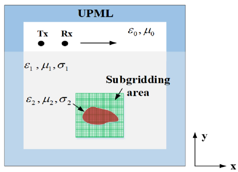
Figure 1: Configuration of the two-dimensional GPR model.

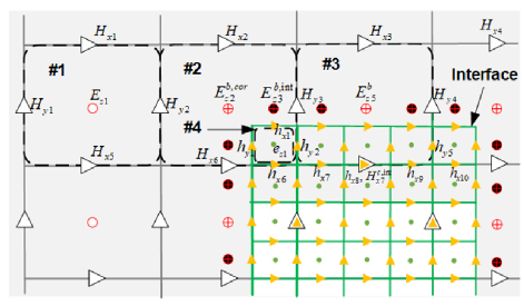
Figure 2: Spatial distributions of the electric field intensity and the magnetic field intensity at grid nodes (take TM${}_{\text{z}}$ wave as example).

A. Overall algorithm of the model

To describe the algorithm principle of the model, the coarse/fine grid size ratio of 3:1 is taken as an example. Figure 2 shows the spatial distributions of the electric field intensity (E or e) and the magnetic field intensity (H or h) at grid nodes. As Fig. 2 shows, the meshes in the model mainly include the coarse mesh nodes (in cell #1), the fine mesh nodes (in cell #4), and the border nodes (in cells #2 and #3). In cell #1, the traditional FDTD method is employed to obtain the transient values of E and H at the coarse nodes. In cell #4, the unconditionally stable explicit FDTD method in lossy media is used to calculate the field quantities of e and h in the fine grids. In cells #2 and #3, the E field is calculated by the H field of a portion of the coarse grids and the h field of a portion of the fine grids. It should be noted that the time steps used in all regions are the same.

Following, we will describe the calculation methods for different regions.

B. Explicit unconditional stable FDTD formulations in cell #4

A two-dimensional (2D) TM${}_z$ wave propagating in a lossy medium is considered. Its Maxwell’s equation in time domain (t) can be written as:

$$\left[\begin{array}{ccc}\hfill \epsilon {\partial }_t+\sigma \hfill & \hfill {\partial }_y\hfill & \hfill -{\partial }_x\hfill \\ \hfill {\partial }_y\hfill & \hfill \mu {\partial }_t\hfill & \hfill 0\hfill \\ \hfill {\partial }_x\hfill & \hfill 0\hfill & \hfill -\mu {\partial }_t\hfill \end{array}\right]\left[\begin{array}{c}\hfill E_z\hfill \\ \hfill H_x\hfill \\ \hfill H_y\hfill \end{array}\right]=0,$$

(1)

where ${\partial }_{\varsigma }$ represents the operator of $\partial \mathrm{/}\partial \varsigma$, $\epsilon$ and $\sigma$ are the dielectric constant and the conductivity of the media, respectively, and $\mu$ is the media’s permeability. The wave equation corresponding to (1) is:

$${\partial }_t^2{E}_z+\frac{\sigma }{\epsilon }{\partial }_t{E}_z-{\partial }_y^2{E}_z/\epsilon \mu -{\partial }_x^2{E}_z/\epsilon \mu =0,$$

(2)

where ${\partial }_{\varsigma }^2$ represents the second-order derivative of $\varsigma$. Let $\tilde{E}={\partial }_y^2{E}_z\mathrm{/}\epsilon \mu +{\partial }_x^2{E}_z\mathrm{/}\epsilon \mu$ and expand $\tilde{E}$ using the difference method to obtain:

$\tilde{E}(i,j)=$	${\displaystyle \frac{1}{\epsilon \mu }}\{{\displaystyle \frac{1}{\mathrm{\Delta }{y}^2}}[E_z(i,j+1)-2E_z(i,j)$
		$+E_z(i,j-1)]+{\displaystyle \frac{1}{\mathrm{\Delta }{x}^2}}[E_z(i+1,j)-$
		$2E_z(i,j)+E_z(i-1,j)]\},$	(3)

where i and j represent the grids in space. The matrix form of (B.) is:

$$\widetilde{\mathit{\text{E}}}=\mathit{\text{ME}}.$$

(4)

Here, M is a sparse matrix representing the operator ${\partial }_y^2\mathrm{/}\epsilon \mu +{\partial }_x^2\mathrm{/}\epsilon \mu$, E=[E${}_z$(0,0), E${}_z$(0,1), E${}_z$(0,2), …, E${}_z$(1,0), E${}_z$(1,1), E${}_z$(1,2), …, E${}_z$(2,0), E${}_z$(2,1), E${}_z$(2,2), …]${}^T$.

Taking $\tilde{E}(1,1)$ as an example, its expansion equation is:

$$\begin{array}{c}{\tilde{E}}^n(1,1)=\frac{1}{\epsilon \mu }[\begin{array}{ccccc}\hfill 0\hfill & \hfill \frac{1}{\mathrm{\Delta }{x}^2}\hfill & \hfill 0\hfill & \hfill \mathrm{\cdots }\hfill & \hfill \frac{1}{\mathrm{\Delta }{y}^2}\hfill \end{array}\hfill \\ \begin{array}{ccccccc}\hfill \frac{-2}{\mathrm{\Delta }{x}^2}+\frac{-2}{\mathrm{\Delta }{y}^2}\hfill & \hfill \frac{1}{\mathrm{\Delta }{y}^2}\hfill & \hfill \mathrm{\cdots }\hfill & \hfill 0\hfill & \hfill \frac{1}{\mathrm{\Delta }{x}^2}\hfill & \hfill 0\hfill & \hfill \mathrm{\cdots }\hfill \end{array}]\mathit{\text{E}}\hfill \end{array}.$$

(5)

Substituting (4) into (2), we have:

$$\frac{{\partial }^2\mathit{\text{E}}}{\partial t^2}+{\mathit{\text{D}}}_{\sigma }\frac{\partial \mathit{\text{E}}}{\partial t}-\mathit{\text{ME}}=0,$$

(6)

with ${\mathit{\text{D}}}_{\sigma }$ the diagonal matrix of element $\sigma \mathrm{/}\epsilon$.

Since E is a vector, the characteristic equation of (6) is:

$$({\lambda }^2+{\mathit{\text{D}}}_{\sigma N\times N}\lambda -{\mathit{\text{M}}}_{N\times N}){\mathit{\text{V}}}_{N\times 1}=0,$$

(7)

where V is the right eigenvector corresponding to each eigenvalue $\lambda$. The quantity of $\lambda$ is 2N (N represents the number of grids), so the corresponding number of columns in V is also 2N [21].

After some manipulations, (7) becomes a typical eigenvalue problem as:

$${\mathit{\text{A}}}_{2N\times 2N}{\mathit{\text{u}}}_i={\lambda }_i{\mathit{\text{u}}}_i,i=1,2,\mathrm{\cdots },2N,$$

(8)

with:

$${\mathit{\text{A}}}_{2N\times 2N}=\left[\begin{array}{cc}\hfill {\mathit{\text{O}}}_{N\times N}\hfill & \hfill {\mathit{\text{I}}}_{N\times N}\hfill \\ \hfill {\mathit{\text{M}}}_{N\times N}\hfill & \hfill -{\mathit{\text{D}}}_{\sigma N\times N}\hfill \end{array}\right]\text{and}{\mathit{\text{u}}}_i=\left[\begin{array}{c}\hfill {\mathit{\text{V}}}_i\hfill \\ \hfill {\lambda }_i{\mathit{\text{V}}}_i\hfill \end{array}\right].$$

(9)

It can be seen that A is determined by space discretization and the size of A will expand as the unknown number increases. A is an asymmetric matrix and does not have orthogonality, so its eigenvalue vector u also does not have orthogonality, and $\lambda$ is the eigenvalueof A.

Usually, the generation of unstable modes comes from space discretization. For example, for an object with a large $\epsilon$ or a fine structure, the explicit FDTD algorithm requires very fine mesh generation. Thus, $\mathrm{\Delta }$x and $\mathrm{\Delta }$y must be very small and subject to CFLcondition [22]:

$$\mathrm{\Delta }t\le \frac{\min (\mathrm{\Delta }x,\mathrm{\Delta }y)}{\sqrt{2{\epsilon }_r}c},$$

(10)

where c is the speed of light. Therefore, $\mathrm{\Delta }$t will become very small. According to the Nyquist sampling theorem, $\mathrm{\Delta }$t only needs to meet $\le 1\mathrm{/}{f}_{\max }$ (f${}_{m\mathit{}a\mathit{}x}$ is the maximum frequency of the incident wave), and the high-frequencies $>$f${}_{m\mathit{}a\mathit{}x}$ corresponding to very small $\mathrm{\Delta }$t is redundant [16]. In terms of (8), if $\mathrm{\Delta }$t is selected beyond the CFL condition, the modes corresponding to eigenvalues that do not meet:

$$\left|{\lambda }_i\right|\le \frac{2}{\mathrm{\Delta }t},$$

(11)

will lead to algorithm instability. In fact, these modes correspond to redundant frequencies. Theoretically, the removal of these unstable modes will not affect the accuracy of the algorithm. Therefore, the key to breaking free from CFL constraints in algorithms lies in being able to find the unstable modes in A and remove them. However, due to the large size of A, directly solving the eigenvalues of A would be time-consuming.

To achieve matrix compression, an orthogonal matrix ${\mathit{\text{F}}}_E^T$ is left multiplied into (7):

$${\mathit{\text{F}}}_E^T\left[\left({\lambda }^2\mathit{\text{I}}+{\mathit{\text{D}}}_{\sigma }\lambda -\mathit{\text{M}}\right)V\right].$$

(12)

According to the property that orthogonal matrix ${\mathit{\text{F}}}_E^T$ has ${\mathit{\text{F}}}_E^T{\mathit{\text{F}}}_E={\mathit{\text{I}}}_r$, (12) can be transformed into:

$$\left({\lambda }^2{\mathit{\text{F}}}_E^T{\mathit{\text{F}}}_E+{\mathit{\text{F}}}_E^T{\mathit{\text{D}}}_{\sigma }{\mathit{\text{F}}}_E\lambda -{\mathit{\text{F}}}_E^T{\mathit{\text{M}}\mathit{\text{F}}}_E\right){\mathit{\text{F}}}_E^T\mathit{\text{V}}=0,$$

(13)

i.e.

$$\left({\lambda }^2{\mathit{\text{I}}}_r+{\mathit{\text{D}}}_{\sigma ,r}\lambda -{\mathit{\text{M}}}_r\right){\mathit{\text{V}}}_r=0,$$

(14)

where ${\mathit{\text{D}}}_{\sigma ,r}={\mathit{\text{F}}}_E^T{\mathit{\text{D}}}_{\sigma }{\mathit{\text{F}}}_E$, ${\mathit{\text{M}}}_r={\mathit{\text{F}}}_E^T{\mathit{\text{MF}}}_E$, ${\mathit{\text{V}}}_r={\mathit{\text{F}}}_E^T\mathit{\text{V}}$.

${\mathit{\text{F}}}_E$ are obtained through preprocessing, and its matrix size is N$\mathrm{\times }$a (a$\mathrm{<}$N). Therefore, the matrix sizes of ${\mathit{\text{D}}}_{\sigma ,r}$, ${\mathit{\text{M}}}_r$, and ${\mathit{\text{V}}}_r$ are correspondingly reduced to a$\mathrm{\times }$a, a$\mathrm{\times }$a, and a$\mathrm{\times }$2N. The eigenvalue problem becomes:

$${\mathit{\text{A}}}_{r2a\times 2a}{\mathit{\text{u}}}_{r2a\times 2N}=\lambda {\mathit{\text{u}}}_{r2a\times 2N},$$

(15)

with:

$${\mathit{\text{A}}}_{r2a\times 2a}=\left[\begin{array}{cc}\hfill {\mathit{\text{O}}}_r\hfill & \hfill {\mathit{\text{I}}}_r\hfill \\ \hfill {\mathit{\text{M}}}_r\hfill & \hfill -{\mathit{\text{D}}}_{\sigma ,r}\hfill \end{array}\right]{\text{and}\mathit{\text{u}}}_{r2a\times 2N}=\left[\begin{array}{c}\hfill {\mathit{\text{V}}}_r\hfill \\ \hfill \lambda {\mathit{\text{V}}}_r\hfill \end{array}\right].$$

(16)

Obviously, the eigenvalues of (15) have not changed, but the scale of matrices $A_r$ and $u_r$ has significantly decreased.

By executing:

$${\mathit{\text{V}}}_{st}={\mathit{\text{F}}}_E{\mathit{\text{V}}}_r,$$

(17)

the eigenvector containing stable modes can be obtained. The size of $V_{st}$ is the same as that of V${}_{\mathrm{r}}$. The stable transient E${}_{\mathrm{s}\mathit{}\mathrm{t}}$(t) can be represented as:

$${\mathit{\text{E}}}_{st}(t)={\mathit{\text{V}}}_{st}\mathit{\text{y}}(t).$$

(18)

Substituting (18) into (2) and performing the central difference scheme on the equation, we have:

$\left(\mathit{\text{I}}+{\displaystyle \frac{\mathrm{\Delta }t}{2}}{\mathit{\text{C}}}_b\right){\mathit{\text{y}}}^{n+1}=$	$\left(2\mathit{\text{I}}+\mathrm{\Delta }{t}^2{\mathit{\text{C}}}_c\right){\mathit{\text{y}}}^n$
		$-\left(\mathit{\text{I}}-{\displaystyle \frac{\mathrm{\Delta }t}{2}}{\mathit{\text{C}}}_b\right){\mathit{\text{y}}}^{n-1}.$	(19)

$C_b$ and $C_c$ are calculated by:

${\mathit{\text{C}}}_b={\left({\mathit{\text{V}}}_{st}^H{\mathit{\text{V}}}_{st}\right)}^{-1}{\mathit{\text{V}}}_{st}^H{\mathit{\text{D}}}_{\sigma }{\mathit{\text{V}}}_{st}.$
${\mathit{\text{C}}}_c={\left({\mathit{\text{V}}}_{st}^H{\mathit{\text{V}}}_{st}\right)}^{-1}{\mathit{\text{V}}}_{st}^H{\mathit{\text{M}}\mathit{\text{V}}}_{st}.$	(20)

Therefore, (B.) can be written as:

$$y^{n+1}=C_d{y}^n+C_e{y}^{n-1},$$

(21)

in which $C_d$ and $C_e$ are given by:

${\mathit{\text{C}}}_d={\left(\mathit{\text{I}}+{\displaystyle \frac{\mathrm{\Delta }t}{2}}{\mathit{\text{C}}}_b\right)}^{-1}\left(2\mathit{\text{I}}+\mathrm{\Delta }{t}^2{\mathit{\text{C}}}_c\right)$
${\mathit{\text{C}}}_e=-{\left(\mathit{\text{I}}+{\displaystyle \frac{\mathrm{\Delta }t}{2}}{\mathit{\text{C}}}_b\right)}^{-1}\left(\mathit{\text{I}}-{\displaystyle \frac{\mathrm{\Delta }t}{2}}{\mathit{\text{C}}}_b\right).$	(22)

Execute (21) and (18) to compute unconditional stable E${}_{\mathrm{s}\mathit{}\mathrm{t}}$(t) and then substitute E${}_{\mathrm{s}\mathit{}\mathrm{t}}$(t) into (1). The value of H${}_{\mathrm{s}\mathit{}\mathrm{t}}$(t) can be obtained simultaneously.

To improve efficiency, V${}_{\mathrm{r}}$ and $\lambda$ are not directly solved but are obtained by iterating FDTD for some steps. The specific method is as described in Algorithm 1.

C. Subgridding scheme in cells #2 and #3

In the subgridding scheme, properly dealing with coupling between the base and fine grid interfaces is crucial because it determines the stability and accuracy of the algorithm. However, the algorithms that can improve accuracy are often complex. In this paper, we adopt the improved separated temporal and spatial interfaces subgridding method to solve the above issues. Due to the application of the unconditional stability technique, both coarse and fine grids use the same time increment, which further reduces the complexity of the algorithm.

Taking the 2D TM wave subgridding interface shown in Fig. 2 as an example: H${}_x$${}_{\mathrm{2}}$, H${}_x$${}_{\mathrm{3}}$, H${}_x$${}_{\mathrm{6}}$, H${}_y$${}_{\mathrm{2}}$, H${}_y$${}_{\mathrm{3}}$, H${}_y$${}_{\mathrm{4}}$ are the magnetic fields of the coarse grid; h${}_x$${}_{\mathrm{1}}$, h${}_x$${}_{\mathrm{6}}$, h${}_x$${}_{\mathrm{7}}$, h${}_x$${}_{\mathrm{8}}$, h${}_x$${}_{\mathrm{9}}$, h${}_x$${}_{\mathrm{10}}$, h${}_y$${}_{\mathrm{1}}$, h${}_y$${}_{\mathrm{2}}$, h${}_y$${}_{\mathrm{5}}$ are the magnetic fields of the fine grid; $E_{z2}^{b,cor}$, $E_{z3}^{b,int}$, $E_{z5}^b$, $H_{x7}^{c,int}$ are the fields of coarse/fine grid interface, in which $E_{z2}^{b,cor}$ is located at the boundary corner. All these fields need to be particularly treated.

According to [20], E${}_z$ on the interface can be solved by:

$$E_z^{n+1}=E_z^n+\frac{\mathrm{\Delta }t}{\mu }\frac{1}{\mathrm{\Delta }S}\sum _i{l}_i{H}_i,$$

(23)

where $\mathrm{\Delta }t$ is the time step of the FDTD method and $\mathrm{\Delta }S$ is the area of a grid. Thus:

$H^{c,int}$ comes from the interpolation of h in the fine grid [20]:

$$H^{c,int}=\sum _{i=1}^{2m-1}\frac{m-\left|m-i\right|}{m^2}{h}_i.$$

(26)

Hence, $H_{x7}^{c,int}$ can be estimated by:

$$H_{x7}^{c,int}=\frac{1}{9}{h}_{x6}+\frac{2}{9}{h}_{x7}+\frac{1}{3}{h}_{x8}+\frac{2}{9}{h}_{x9}+\frac{1}{9}{h}_{x10}.$$

(27)

Use $E_z^{b,int}$ to update h${}_x$ and h${}_y$ on the boundary. $E_z^{b,int}$ is calculated through linear interpolation. Taking $E_{z3}^{b,int}$ as an example:

$$E_{z3}^{b,int}=\frac{2}{3}{E}_{z2}^{b,cor}+\frac{1}{3}{E}_{z5}^b.$$

(28)

For ease of understanding, suppose that the current time step is n and all fields are known. We summarize the update process of the proposed subgridding scheme into the following steps:

Step #1: Calculate $E^{n+1}$ and $H^{n+\frac{3}{2}}$(such as H${}_x$${}_{\mathrm{2}}$, H${}_x$${}_{\mathrm{3}}$, H${}_x$${}_{\mathrm{6}}$, H${}_y$${}_{\mathrm{3}}$, H${}_y$${}_{\mathrm{4}}$) for coarse grids by using the traditional FDTD method.

Step #2: Calculate $e^{n+1}$ and $h^{n+\frac{3}{2}}$(such as h${}_x$${}_{\mathrm{6}}$, h${}_x$${}_{\mathrm{7}}$, h${}_x$${}_{\mathrm{8}}$, h${}_x$${}_{\mathrm{9}}$, h${}_x$${}_{\mathrm{10}}$, h${}_y$${}_{\mathrm{2}}$, h${}_y$${}_{\mathrm{5}}$) for fine grids by using the explicit unconditional stable FDTD formulations.

Step #3: Substitute (27) into (24) to obtain $E_{z5}^{b,n+1}$, and substitute (24), (C.), into (28) to obtain $E_{z3}^{b,int,n+1}$. Thus, the fields on the coarse/fine grids interface can be updated accordingly.

It should be noted that the subgridding scheme and the unconditional stable algorithm above are analyzed and derived based on TM${}_z$ waves. The proposed method in this paper is applicable for 2D GPR numerical simulation in TM mode.

III. NUMERICAL RESULTS

A. Accuracy

To demonstrate the accuracy of this proposed subgridding unconditional stable algorithm, a square object (${\epsilon }_{r2}=$5, ${\mu }_{r2}=$1, ${\sigma }_2=$0.02 S/m) in a homogeneous medium (${\epsilon }_{r1}=$3, ${\mu }_{r1}=$1, ${\sigma }_1$=0.1 S/m) is illustrated (see Fig. 3). The object has a size of 0.21$\times$0.21 m with a center located at (0.675 m, 0.495 m). It is illuminated by a TM${}_z$ wave in the form of:

$$J_z=\delta (x-x_0,y-y_0)e^{(-{((t-t_0)\mathrm{/}{t}_d)}^2)}.$$

(29)

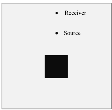
Figure 3: Model for algorithm accuracy verification.

Here, (x${}_{\mathrm{0}}$, y${}_{\mathrm{0}}$) is the location of the source, $\delta (x-x_0,y$$-y_0)=1\mathrm{/}(\mathrm{\Delta }x\mathrm{\Delta }y)$, $t_0=0.9\mathrm{/}{f}_c$, $t_d=t_0\mathrm{/}4$, and f${}_c$=5 MHz. The source is placed at (0.66 m, 0.9 m), and the receiver is located at (0.66 m, 1.2 m).

Two sizes of grids with $\mathrm{\Delta }{l}_{base}=$30 mm and $\mathrm{\Delta }{l}_{fine}=$10 mm are adopted. Their size ratio is 3. A temporal step of CFL stability condition of uniform base grids is chosen, which is three times beyond CFL condition of uniform fine grids. The total number of the eigenmodes is 800, of which 773 unstable eigenmodes need to be removed. Furthermore, we also compute the numerical problem when the size ratio increases to 5, 15, 25, 75, and the removed eigenmodes are 2287, 21621, 60542, 549121, with the total eigenmodes number 2312, 21632, 60552, 549152. When selecting different grid size ratios, the number of grids applying unconditional stable algorithm vary, so the total eigenmodes number will be different and this leads to different stable eigenmodes size. On the other side, error e${}_{\mathrm{1}}$, e${}_{\mathrm{2}}$ and FDTD step n in the unconditional stable algorithm also affects the number of stable eigenmodes. In this problem, we choose the parameters e${}_{\mathrm{1}}$, e${}_{\mathrm{2}}$, n in the procedure of finding stable eigenmodes with e${}_{\mathrm{1}}\mathrm{=}$10${}^{-4}$ and e${}_{\mathrm{2}}\mathrm{=}$10${}^{-}$${}^3$ with n$\mathrm{=}$3 (grid size ratio equals 3), e${}_{\mathrm{2}}\mathrm{=}$10${}^{-}$${}^2$ with n$\mathrm{=}$5 (grid size ratio equals 5), e${}_{\mathrm{2}}\mathrm{=}$10${}^{-2}$ with n$\mathrm{=}$15 (grid size ratio equals 15), e${}_{\mathrm{2}}\mathrm{=}$10${}^{-}$${}^4$ with n $=$25 (grid size ratio equals 25), e${}_{\mathrm{2}}\mathrm{=}$10${}^{-4}$ with n$\mathrm{=}$30 (grid size ratio equals 75).

The transient E${}_z$(t) at the receiver computed using the proposed algorithm are compared with the results of traditional FDTD method based on uniform grid ($\mathrm{\Delta }{l}_{fine}$) and traditional subgridding approach. As shown in Fig. 4, the proposed method with ratio=3 and 5 has the best agreement in our simulation; a larger ratio will lead to some accuracy loss. Although there is a gradually increasing error when ratio$=$15, 25, 75, it indicates that the proposed method is feasible when we use a large ratio. This proposed method will have more advantages in multi-scale electromagnetic problem simulation.

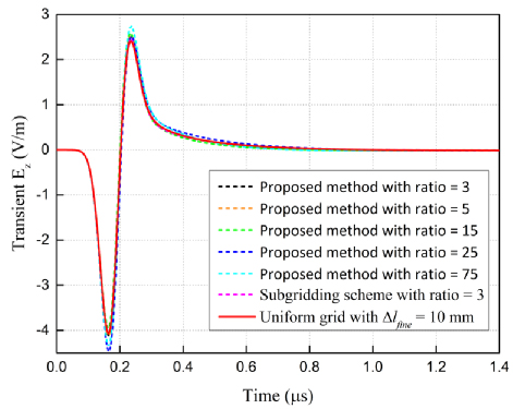
Figure 4: Electric field computed by conventional FDTD, subgridding FDTD, and subgridding unconditional stable algorithm.

To measure the accuracy of the algorithm, a relative error is defined as:

$$\mathrm{Error}(t)=\frac{\left|E_z(t)-E_{z,ref}(t)\right|}{{\left|E_{z,ref}(t)\right|}_{\max }}\times 100\%.$$

(30)

The reference solution $E_{z,ref}(t)$ is obtained by conventional FDTD with $\mathrm{\Delta }{l}_{fine}$. The relative errors of the traditional subgridding FDTD and the proposed method are shown in Fig. 5. It can be seen that the relative error of the proposed method with ratio$=$3 is less than 3%, and there is only a slight difference when ratio$=$3 and 5. It must be pointed out that when selecting an appropriate grid size ratio, the computational accuracy of the proposed approach is slightly lower than the subgridding scheme.

Table 1 lists the computational resource consumption of three methods. From Table 1, the following observations are made:

• The number of unknowns in the proposed method with ratio $=$ 3, 5, 15 is 0.19, 0.22, 0.64 compared to the conventional FDTD. The proposed method with ratio $=$ 3 reduces memory cost by 52.48% and saves computational time by 84.84% compared to that of conventional FDTD. The proposed method with ratio$=$5, 15 has advantages in terms of time consumption.

• Compared to the subgridding scheme, the proposed method with ratio $=$ 3, 5 reduces memory cost by 73.33%, 20%, and saves computational time by 53.07%, 50.27%. The proposed method with ratio=15 has advantages in terms of time consumption.

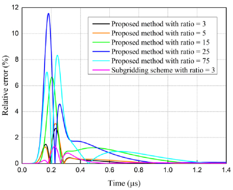
Figure 5: Relative error of the traditional subgridding scheme and the proposed subgridding unconditional stable algorithm.

Table 1: Computational resource consumption of the three methods

Method	Grid Ratio	Grid Number	Memory (MB)	Time(s)
FDTD	1	70840	1.01	62.06
Subgridding Scheme	3	13364	1.80	20.05
Proposed Method	3	13364	0.48	9.41
	5	15716	1.44	9.97
	15	45116	1.90	25.06
	25	103916	5.32	84.68
	75	838916	130.13	10825.27

In our experiment, as the grid size ratio increases from 3 to 75, the CPU time of the preprocessing procedure to find stable eigenmodes is 0.33 s, 0.49 s, 0.87 s, 1.99 s, 125.89 s, respectively. It is clear that the preprocessing time only accounts for a small portion of the total time in Table 1. In this numerical example, when we select inappropriate parameter e${}_{\mathrm{1}}$, e${}_{\mathrm{2}}$ and step size n, the main resource consumption increment will come from the preprocess of finding the stable vector V${}_{\mathrm{r}\mathrm{,}\mathrm{s}\mathit{}\mathrm{t}}$. In our experience, e${}_{\mathrm{1}}$ is on the order of 10${}^{-4}$, e${}_{\mathrm{2}}$ is 10${}^{-}$ ${}^4$$\sim$10${}^{-2}$, and n usually equals the grid size ratio when it is not too large.

B. GPR model

Next, we apply the algorithm to the 2D GPR model, as Fig. 6 shows, while keeping the time step and spatial step unchanged. A lossy square (${\epsilon }_{r1}=$2, ${\mu }_{r1}=$1, ${\sigma }_1=$0.97 S/m) is buried under the dispersive soil (${\epsilon }_{r0}=$4, ${\mu }_{r0}=$1, ${\sigma }_0=$0.004 S/m). The size of the simulation domain is 3$\times$3.6 m, with the object located at a depth of 1.89 m below the surface and the center at (1.245 m, -1.965 m). Its scale is 0.15$\times$0.15 m. Tx and Rx are placed at (0.48 m, 0.09 m) and (2.46 m, 0.09 m), respectively.

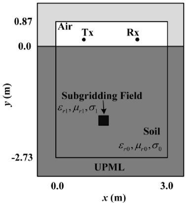
Figure 6: Two-dimensional GPR model.

A TM wave is excited by the z-component of a current source J${}_z$(t) with first derivative of the Blackman-Harris pulse as:

$$J_z(t)=\{\begin{array}{c}-\frac{2\pi }{T_s}\sum _{n=0}^3{a}_{n}n\sin \left(\frac{2\pi nt}{T_s}\right),\mathrm{\hspace{0.33em}\hspace{0.33em}0}<t<T_s\hfill \\ 0,otherwise\hfill \end{array},$$

(31)

with f${}_c$$\mathrm{=}$100 MHz, T${}_s$$\mathrm{=}$0.9/f${}_c$, a${}_{\mathrm{0}}\mathrm{=}$0.3532, a${}_{\mathrm{1}}\mathrm{=}$-0.488, a${}_{\mathrm{2}}\mathrm{=}$0.145, and a${}_{\mathrm{3}}\mathrm{=}$-0.0102.

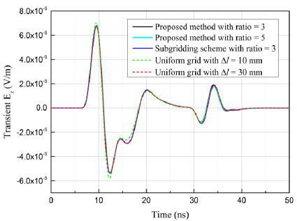
Figure 7: Comparison of the electric fields computed by different methods.

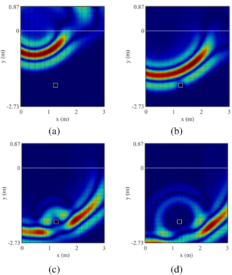
Figure 8: Time snapshot of electric field amplitude in the computational domain: (a) n$=$150, (b) n$=$220, (c) n$=$290, and (d) n$=$330.

Figure 7 shows comparisons of the transient E${}_z$(t) at Rx. It can be seen that the proposed method agrees well with the results of other methods. In the proposed algorithm, we compute the problem with grid ratio 3 and 5, scale of coefficient matrix A is 392$\times$392, 1152$\times$1152, and number of stable modes is 7 and 3. In the unconditional stable process, parameter e${}_{\mathrm{1}}\mathrm{=}$10${}^{-4}$, e${}_{\mathrm{2}}\mathrm{=}$10${}^{-2}$, and step size n$\mathrm{=}$3, 5.

Figure 8 shows time snapshots of the electric field amplitudes in the computational domain at n$\mathrm{=}$150, 220, 290, and 330, where the Tx and Rx antennas arestatic.

In B-Scan simulation, Tx is moved from (0.09 m, 0.09 m) to (2.91 m, 0.09 m), with a spatial increment of 0.06. Rx also moves with Tx, and the distance between them is always 0.09 m in the x-axis direction. Figure 9 shows the contour of the echo z-component of the electric field received by Rx.

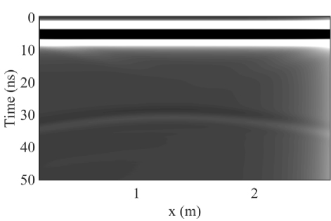
Figure 9: Contour of the echo electric field received by Rx.

Computational resource consumption of the three methods in the GPR simulation are listed in Table 2. The efficiency of the proposed algorithm has been validated again. It can be seen that the proposed method has superiority in memory consuming compared to the other two methods with acceptable time increment and showing its potential in GPR simulation.

Finally, we carried out an experiment to test the performance of the proposed method when simulated in media with different electrical properties. We changed the buried object by selecting material parameter $\epsilon$${}_r$${}_1=$2, 4, 8, and $\sigma$${}_1=$0 S/m, 4 S/m, 16 S/m, respectively. There are no obvious variations in memory cost and time consumption, and the accuracy is also stable with relative error below 6%. Long-term instability will occur from the interface of the base and fine grid when low $\epsilon$${}_r$${}_1$ and $\sigma$${}_1$ are chosen, and can be a direction to improve the proposed method.

Table 2: Computational resource consumption of the three methods

Method	Grid Ratio	Grid Number	Memory (MB)	Time (s)
FDTD with 10	1	362005	2.47	1342.11
$\mathrm{\Delta }l=$ (mm) 30	1	49365	0.63	12.02
Subgridding Scheme	3	49985	1.98	12.75
Proposed Method	3	49985	1.09	13.67
	5	51185	1.47	13.05

IV. CONCLUSION

In this paper, an explicit unconditionally stable technique is introduced into the subgridding 2D-FDTD approach and applied in GPR modeling with TM mode. A subgridding algorithm with separated temporal and spatial interfaces is proposed to solve the multiscale problem. The unconditional stable algorithm can find all the stable eigenmodes to keep numeric stability without compromising accuracy when the time step does not meet CFL conditions, and the numerical results demonstrate its good performance in terms of accuracy. In GPR simulation, this proposed method’s potential in solving multiscale problems is demonstrated.

ACKNOWLEDGMENT

The authors wish to acknowledge the support of the National Natural Science Foundation of China (Grants #61761017).

REFERENCES

[1] G. Bozza, C. Estatico, M. Pastorino, and A. Randazzo, “Application of an inexact-Newton method within the second-order born approximation to buried objects,” IEEE Geoscience & Remote Sensing Letters, vol. 4, pp. 51-55, 2007.

[2] Y. Altuncu, “A numerical method for electromagnetic scattering by 3-D dielectric objects buried under 2-D locally rough surfaces,” IEEE Transactions on Antennas and Propagation, vol. 63, no. 8, pp. 3634-3643, 2015.

[3] K. Yee, “Numerical solution of initial boundary value problems involving Maxwell’s equations in isotropic media,” IEEE Trans. Antennas Propag., vol. 14, no. 3, pp. 302-307, 1966.

[4] A. Taflove and S. C. Hagness, Computational Electrodynamics: The Finite-Difference Time-Domain Method. Boston, MA: Artech House, 2000.

[5] D. T. Prescott and N. V. Shuley, “A method for incorporating different sized cells into the finite-difference time-domain analysis technique,” IEEE Microwave and Guided Wave Letters, vol. 2, no. 11, pp. 434-436, 1992.

[6] S. S. Zivanovic, K. S. Yee, and K. K. Mei, “A subgridding method for the time-domain finite-difference method to solve Maxwell’s equations,” IEEE Transactions on Microwave Theory and Techniques, vol. 39, no. 3, pp. 471-479, 1991.

[7] M. J. White, M. F. Iskander, and Z. Huang, “Development of a multigrid FDTD code for three-dimensional applications,” IEEE Transactions on Antennas and Propagation, vol. 45, no. 10, pp. 1512-1517, 1997.

[8] J. Yan and D. Jiao, “An unsymmetric FDTD subgridding algorithm with unconditional stability,” IEEE Transactions on Antennas and Propagation, vol. 66, no. 8, pp. 4137-4150, 2018.

[9] H. Al-Tameemi, J. P. Berenger, and F. Costen, “Singularity problem with the one-sheet Huygens subgridding method,” IEEE Transactions on Electromagnetic Compatibility, vol. 99, pp. 1-4, 2016.

[10] J. Hartley, A. Giannopoulos, and C. Warren, “A Huygens subgridding approach for efficient modelling of ground penetrating radar using thefinite-difference time-domain method,” in 2018 17th International Conference on Ground Penetrating Radar (GPR), 2018.

[11] N. V. Venkatarayalu, R. Lee, Y.-B. Gan, and L.-W. Li, “A stable FDTD subgridding method based on finite element formulation with hanging variables,” IEEE Transactions on Antennas & Propagation, vol. 55, no. 3, pp. 907-915, 2007.

[12] K. Xiao, D. J. Pommerenke, and J. L. Drewniak, “A three-dimensional FDTD subgridding algorithm with separated temporal and spatial interfaces and related stability analysis,” IEEE Transactions on Antennas and Propagation, vol. 55, no. 7, pp. 1981-1990, 2007.

[13] N. Diamanti and A. Giannopoulos, “Implementation of ADI-FDTD subgrids in ground penetrating radar FDTD models,” Journal of Applied Geophysics, vol. 67, no. 4, pp. 309-317, 2009.

[14] M. R. Cabello, L. D. Angulo, J. Alvarez, I. D. Flintoft, S. Bourke, J. F. Dawson, R. G. Martin, and S. G. Garcia, “A hybrid Crank-Nicolson FDTD subgridding boundary condition for lossy thin-layer modeling,” IEEE Transactions on Microwave Theory & Techniques, vol. 65, no. 5, pp. 1397-1406, 2017.

[15] M. Zhou, Z. David Chen, W. Fan, X. Bo, and W. Wei, “A subgridding scheme with the unconditionally stable explicit FDTD method,” in IEEE MTT-S International Conference on Numerical Electromagnetic & Multiphysics Modeling & Optimization, Beijing, China, pp. 1-3, 2016.

[16] M. Gaffar and D. Jiao, “An explicit and unconditionally stable FDTD method for electromagnetic analysis,” IEEE Transactions on Microwave Theory and Techniques, vol. 62, no. 11, pp. 2538-2550, 2014.

[17] J. Yan and D. Jiao, “Symmetric positive semidefinite FDTD subgridding algorithms for arbitrary grid ratios without compromising accuracy,” IEEE Transactions on Microwave Theory and Techniques, vol. 65, no. 12, pp. 5084-5095, 2017.

[18] K. Zeng and D. Jiao, “Symmetric positive semi-definite FDTD subgridding algorithms in both space and time for accurate analysis of inhomogeneous problems,” IEEE Transactions on Antennas and Propagation, vol. 68, no. 4, pp. 3047-3059, 2020.

[19] X.-K. Wei, X. Zhang, N. Diamanti, W. Shao, and C. D. Sarris, “Subgridded FDTD modeling of ground penetrating radar scenarios beyond the courant stability limit,” IEEE Transactions on Geoscience & Remote Sensing, vol. 12, pp. 1-10, 2017.

[20] Z. Ye, C. Liao, X. Xiong, and M. Zhang, “A novel FDTD subgridding method with improved separated temporal and spatial subgridding interfaces,” IEEE Antennas and Wireless Propagation Letters, vol. 16, pp. 1011-1015, 2017.

[21] F. Tisseur and K. Meerbergen, “The quadratic eigenvalue problem,” SIAM Review, vol. 43, no. 2, pp. 235-286, 2001.

[22] R. Courant, K. Friedrichs, and H. Lewy, “Über die partiellen differenzengleichungender mathematis-chen physik [in German],” Math. Ann., vol. 100, no. 1, pp. 32-74, 1928.

BIOGRAPHIES

Xiao Yan Zhang received the B.S. degree in applied physics and the M.S. degree in physical electronics from Yunnan University, Kunming, China, in 2001 and 2004, respectively, and the Ph.D. degree in electromagnetic field and micro-wave technology from the Institute of Electronics, Chinese Academy of Sciences, Beijing, China, in 2007. Her research interests include electromagnetic computation and antenna design.

Rui Long Chenwas born in Hengyang, Hunan, China, in 1996. He received the B.S. degree in communication engineering from Beijing Union University, Beijing, China, in 2018, and the M.S. degree in communication engineering from East China Jiao Tong University, Nanchang, China, in 2021. Currently, he is pursuing the Ph.D. degree in Xiangtan University, Xiangtan, China. His research interests focus on electromagnetic computation and numerical methods of partial differential equations.

ACES JOURNAL, Vol. 40, No. 6, 499–507
doi: 10.13052/2024.ACES.J.400602
© 2025 River Publishers