Convolutional Neural Networks Aided Reinforcement Learning for Accelerated Optimization of Antenna Topology

Jiangling Dou $^{1,2}$ , Hao Gong $^{2}$ , Shuaibing Wei $^{2}$ , Haokang Chen $^{2}$ , Yujie Chen $^{2}$ , Tao Shen $^{3}$ , and Jian Song $^{1,2}$

¹Yunnan Key Laboratory of Computer Technologies Application
Kunming University of Science and Technology, Kunming 650500, China
jianglingdou@kust.edu.cn, songjian@kust.edu.cn

²School of Information Engineering and Automation
Kunming University of Science and Technology, Kunming 650500, China
20222104053@stu.kust.edu.cn, weishuaibing@stu.kust.edu.cn, haokangchen@stu.kust.edu.cn, chenyujie@stu.kust.edu.cn

³College of Mechanical and Electrical Engineering
Yunnan Electromechanical Vocational and Technical College, Kunming 650500, China
shentao@kust.edu.cn

Submitted On: October 28, 2024; Accepted On: January 20, 2025

ABSTRACT

A machine learning (ML) framework is proposed to achieve the automatic and rapid optimization of antenna topologies. A convolutional neural network (CNN) is utilized as a surrogate model (SM) and is combined with reinforcement learning (RL) algorithms. Specifically, the RL agent interacts with simulation software to learn. Data accumulated from electromagnetic (EM) simulations are used to train the SM. The CNN-based SM predicts antenna performance based on the topology of the antenna. Subsequently, the SM replaces EM simulations within the RL training environment. The RL agent interacts with the CNN-based SM to search for the optimal topology. This approach significantly reduces dependence on time-consuming EM simulations. To validate the effectiveness of the optimization method, a center-fed microstrip patch antenna is optimized. Simulation results demonstrate that, compared to other optimization methods, impedance bandwidth is improved, while the number of simulation samples and optimization time are significantly reduced.

Index Terms: Convolutional neural network (CNN), machine learning (ML), microstrip antenna, reinforcement learning (RL), surrogate model (SM), topology optimization.

I. INTRODUCTION

Modern electromagnetic (EM) design typically relies on extensive EM simulation software. Consequently, it poses significant challenges to engineers due to the time-consuming and intricacies of the process. To address these challenges and alleviate the burden on human engineers, machine learning (ML) has been introduced into antenna design. Various ML models, such as gaussian process regression (GPR) [1], support vector machines (SVM) [2], and convolutional neural networks (CNN) [3, 4], have been employed as surrogate models (SMs). These models enable the rapid prediction of antenna performance responses, thereby significantly reducing the calculation costs associated with EM simulations. Additionally, CNN [5] and artificial neural networks (ANN) [6] have been utilized to design inverse models for predicting antenna structural parameters. Genetic algorithms (GA) [7] and particle swarm optimization (PSO) [8] have also been applied to optimize antenna topologies. However, these ML-assisted methods exhibit considerable limitations. For instance, SMs require human intervention to provide prior conditions for training samples and metaheuristic algorithms demand extensive population iterations.

To further reduce dependence on prior domain knowledge and achieve automated topology design, reinforcement learning (RL) is utilized to establish optimal models for antenna topology optimization. RL interacts with the environment and dynamically adjusts the agent’s actions. This makes RL suitable for solving complex decision-making tasks in antenna design. In previous studies, RL has been applied to edge structure design of antennas [9] and the optimization of complex antenna arrays [10]. However, traditional RL methods necessitate a substantial dataset for achieving satisfactory performance.

A RL-based method is proposed to optimize antenna topologies and accelerate the optimization process. The method integrates CNN into the RL framework. Initially, the RL framework learns from interactions with full-wave simulation software. Actions are taken by the RL agent to maximize reward signals. This process leads to the identification of optimal antenna topologies. Subsequently, the acquired data are used to train the CNN. The trained CNN serves as a SM, replacing the simulation software. Antenna performance is predicted by the SM based on the topology. This allows RL to interact with the CNN instead of relying on expensive EM computations. Efficient automated design optimization is thus achieved.

A microstrip antenna is optimized using this method. Simulation results indicate that, compared to other ML algorithms, the antenna achieves a wider impedance bandwidth with reduced optimization time and without prior knowledge intervention.

II. INTRODUCED METHODOLOGY

A. Optimization process of the introduced method

The workflow of the introduced method is illustrated in Fig. 1. The entire design process is divided into three stages. In the data collection stage, state, action, and reward are defined. The RL-based agent generates a topology structure as an action derived from the initial state, and transmits it to the simulation software. The software performs simulations on the provided topology structure, generating the corresponding antenna performance as the new state. The agent interacts with full-wave simulation software to learn. A training dataset that correlates antenna topologies with their performance is generated. The collected data are primarily used to train the RL algorithm. Additionally, the data are repeatedly used in the second stage to train the CNN. In this process, antenna topologies serve as inputs to the CNN, while performance parameters are used as outputs. In the RL stage, when the CNN is trained, the RL algorithm stops interacting with the simulation software and interacts directly with the CNN. In this scenario, a significant quantity of training data can be gathered swiftly, which aids in the rapid convergence of the RL-based model. The deep deterministic policy gradient (DDPG) algorithm is employed as the RL algorithm due to its suitability for handling spatial problems of high dimension and continuity. During the deployment stage, the trained RL model is used to optimize antenna topologies. The RL model continuously adjusts the antenna topologies. If the output samples do not meet the design requirements, they are reintroduced into the CNN’s training dataset. Retraining is performed until the desired design objectives are achieved.

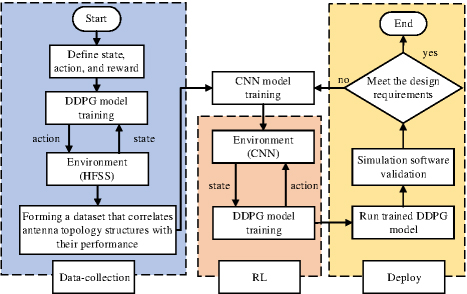
Figure 1: Flowchart of the algorithm optimization.

B. Convolutional neural networks

CNN is a mathematical structure, typically composed of three types of layers: convolutional layers, pooling layers, and fully connected layers. In this paper, CNN is employed as SM to replace simulation software. The input to the CNN is an image of the antenna topology, and the output is a performance curve.

The CNN architecture employed is shown in Fig. 2. The initial two layers focus on extracting features, and the third layer maps these features to produce the final output, such as antenna performance parameters corresponding to the respective topologies. Convolutional layers are fundamental components of CNN. They generally comprise linear as well as nonlinear operations, including convolution and activation.

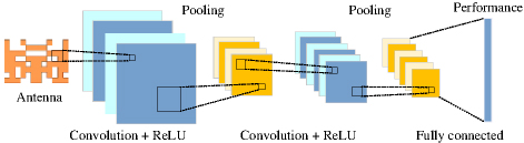
Figure 2: CNN framework diagram.

The convolution operation involves applying a set of filters (kernels) to the input tensor. Each filter convolves over the width and height of the input tensor, generating a two-dimensional activation map. Mathematically, for input X and filter W, the convolution operation can be formulated as:

Z_{i, j} = {(X * W)}_{i, j} = \sum_{m} \sum_{n} X_{i + m, j + n} W_{m, n},

(1)

where Z represents the output feature map, and i and j denote the spatial dimensions of the output.

To enhance nonlinearity, the output of the convolution operation is passed through an activation function. A rectified linear unit (ReLU) activation function is employed, which is defined as follows:

ReLU (z) = \max (0, z) .

(2)

After the convolutional layer, pooling layers are employed to reduce the spatial dimensions of the feature maps. In max pooling, the maximum value within a specified window is selected to down sample the feature maps. This can be expressed as:

Z_{i, j}^{'} = \max_{m, n} Z_{s i + m, s j + n},

(3)

where s is the stride of the pooling operation. The output of the final pooling layer is flattened and passed through one or more fully connected layers. In the fully connected layers, each neuron is connected to every neuron in the preceding layer. The final output layer for predicting antenna performance can be described as follows:

y = W \cdot X + b,

(4)

where W is the weight matrix, X is the input vector from the final pooling layer, and b is the bias vector.

To balance computational cost and modeling capability, the employed CNN consists of two stacked convolutional and pooling layers, followed by a fully connected layer. Through this architecture, the model effectively extracts features and maps them to the final output for antenna performance prediction.

C. DDPG algorithm

The DDPG [11] algorithm is illustrated in Fig. 3. It is implemented using two neural networks. The actor network generates a probability matrix (a $_{p r e}$ ) of antenna topologies based on the current state (s). The a $_{p r e}$ represents the probability of metal presence in each grid cell, with each element ranging from 0 to 1. This probability matrix is converted into an action (a) through the image mapping topology (IMT) module and is then sent to the environment, as shown in Fig. 4. The critic network takes the current state (s) and the action (a) generated by the IMT as inputs, then produces the discounted cumulative reward of the current policy.

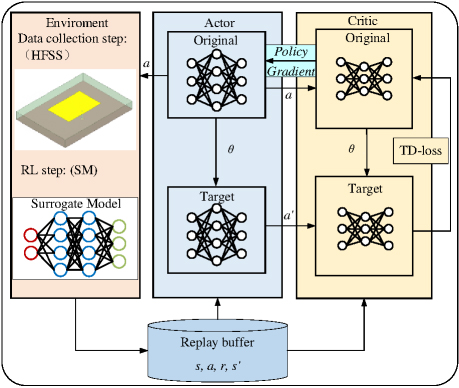
Figure 3: DDPG algorithm framework diagram.

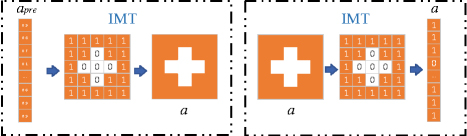
Figure 4: Image mapping topology.

To enhance the stability of the algorithm and ensure its convergence, target networks and replay buffer are employed in DDPG. The target network provides slowly updated parameters as targets, ensuring a smoother convergence path for DDPG. Experiences, including states, actions, rewards, and next states (s, a, r, s $^{'}$ ), are stored in the replay buffer for subsequent training. The replay buffer aids in disrupting the relationship between successive experiences, thereby improving learning efficiency. Throughout the DDPG training process, temporal difference errors (TD-loss) are used as learning signals, and the network parameters ( $θ$ ) are updated through gradient descent.

The implementation of the DDPG algorithm requires states, actions, and rewards to be predefined. The specifics are detailed below.

(1) state: At time step t, the state s $_{t}$ consists of the reflection coefficients S $_{11 t}$ :

s_{t} = (S_{11 t}) .

(5)

(2) action: At time step t, the action a $_{t}$ is represented by the matrix of the antenna topology:

a_{t} = f (a_{p r e (t)}) = {\begin{matrix} 1, a_{i} \geq 0.5 \\ 0, a_{i} < 0.5 \end{matrix} = (a_{t 1}, a_{t 2}, \dots, a_{t n}) .

(6)

(3) reward: B $_{t}$ represents the number of frequencies within the 1.9-3 GHz range that are below $-$ 10 dB. The magnitude of the reward is proportional to the bandwidth B $_{t}$ variation. The value of the threshold B $_{t h r e}$ should be flexibly adjusted according to specific problems and requirements:

r (s_{t}, a_{t}) = {\begin{matrix} (B_{t} - B_{t - 1}) / B_{t h r e}, B_{t} \geq B_{t h r e} \\ - 0.1, B_{t} < B_{t h r e} B_{t} \geq B_{t - 1} \\ - 1, o t h e r w i s e . \end{matrix}

(7)

The reward function defines the immediate reward obtained by the agent when executing a specific action in a particular state. The primary objective of the agent is to optimize its action strategy by maximizing the discounted cumulative reward. The Q-function is provided in [12]:

Q (s_{t}, a_{t}) = E [\sum_{k = 0}^{\infty} γ^{k} r_{t + k + 1} | s_{t}, a_{t}] .

(8)

The Q-function is defined as the expected cumulative reward for a given state-action pair, which takes temporal discount into consideration. The discount factor $γ$ is set between 0 and 1, and is used to adjust the relative importance of immediate rewards and future rewards.

III. APPLICATION EXAMPLES

To facilitate comparison with other ML methods, a microstrip patch antenna is employed as an example to validate the optimization efficiency of the introduced method. The structure of the microstrip patch antenna is shown in Fig. 5. The substrate is made of FR4 material with a thickness of 15 mm and a dielectric constant of 4.4. The width and length of the substrate (W $_{1}$ and L $_{1}$ ) are 110 mm and 150 mm, respectively. The patch has a width (W $_{2}$ ) of 48 mm and a length (L $_{2}$ ) of 72 mm.

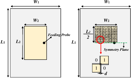
Figure 5: Center-fed microstrip patch antenna structure. The patch is symmetrically divided into 46 binary (0/1) grids, where 1 indicates the presence of metal and 0 indicates its absence. To ensure the electrical connectivity of the metal patch, the edge lengths of the sub-patches are increased by 0.2 mm.

To enable RL to interact with the environment while exploring antenna topologies, an IMT module is incorporated. This module performs gridding of the antenna topology and converts it into corresponding matrix for input into the RL agent. Additionally, it transforms the probability matrix of topology into an image to be input into the environment, as shown in Fig. 4. To maintain a consistent connection between the probe and the patch, the four units connected to the probe are kept unchanged. Furthermore, structural symmetry is enforced along the symmetric plane to avoid high cross-polarization.

As illustrated in Fig. 5, the quantity of topology structure pixels to be determined is 46. The optimization objective is to broaden the bandwidth of the reflection coefficient B $_{t}$ . The frequency step is set to 0.01, and the B $_{t h r e}$ is established at 50. The RL agent continuously interacts with the environment to ascertain the presence of metal in these 46 pixels. Initially, the RL agent interacts with the simulation software, with each topology simulation requiring approximately one minute. Upon collecting 100 samples, the interaction-generated data are then used to train the CNN model, with a training time of 1.2 minutes. As the dataset for the CNN model gradually increases, the prediction accuracy of model continually improves. Once the CNN model training is complete, the CNN model replaces the simulation software within the environment, enabling rapid predictions of the EM responses of corresponding topology. Subsequently, the RL agent interacts with the CNN model, continuously maximizing reward signals to identify the optimal topology structure. The optimization time for each topology is reduced to merely three seconds, with the quantity of learning iterations set to 500 generations. Importantly, although the predictive capability of CNN model enhances with an increasing number of iterations, the algorithm generally operates without the CNN containing sufficient data for predictions. Typically, a SM established with high prediction accuracy requires a significant number of simulations. Additionally, multiple deep network architectures are needed to achieve the desired level of precision. However, the CNN model developed within the RL framework is constructed with a shallow network structure and trained on a limited dataset. This approach helps guide the optimization process towards specified design. The optimized antenna topology and photograph of the manufactured antenna is presented in Fig. 6 and comparative optimization results are shown in Fig. 7 (a).

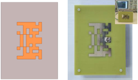
Figure 6: Optimized topology structure of the microstrip antenna and photograph of the manufactured antenna.

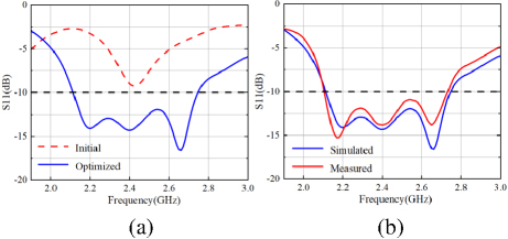
Figure 7: (a) Initial and optimized results and (b) measured and simulated results of S11 for the antenna.

IV. MEASUREMENT AND COMPARISON

The simulation and measurement results are presented in Fig. 7 (b). The impedance bandwidth is 2.1-2.73 GHz, but there are some disparities. These discrepancies may be attributed to manufacturing and installation errors, such as deviations in material thickness, welding position, and tin soldering, which can somewhat impact antenna performance.

The proposed method is compared with several ML-based approaches, as shown in Table 1. Compared to metaheuristic algorithm-based methods [12–14], the proposed method exhibits superior local search capabilities and higher optimization efficiency. Metaheuristic algorithms require the evaluation of each individual in the population and the use of EM simulation software for verification. This process is highly time-consuming. Moreover, the efficiency of metaheuristic algorithms is constrained by the initial population; better initial populations lead to higher optimization efficiency. In contrast, RL obtains feedback through continuous interaction with the environment. This endows RL with strong decision-making capabilities, allowing it to dynamically optimize strategies and progressively guide the optimization toward better solutions. Additionally, RL effectively utilizes existing data through experience replay and policy improvement, thereby reducing the need for expensive simulation samples.

Table 1: Comparison information with other algorithms

Refs.	Optim. Method	Samples	Time	Design Space	Auto Level
[3]	CNN	1970	Not Given	8 $\times$ 6	Semi-Auto
[4]	CNN	625	Not Given	4 params	Semi-Auto
[5]	DCNN	1200	39.62 h	28 params	Semi-Auto
[13]	EGO	2600	43 h	(8 $\times$ 6) $-$ 2	Full-Auto
[14]	BBSO	2500	Not Given	(8 $\times$ 6) $-$ 2	Full-Auto
[15]	BPSO	1000	17.94 h	(8 $\times$ 6) $-$ 2	Full-Auto
CNN-BPSO	254	9.62 h	(8 $\times$ 6) $-$ 2	Semi-Auto
This work	Trial and Error	6400	179 h	(8 $\times$ 6) $-$ 2	Manual
GA	3500	53 h	(8 $\times$ 6) $-$ 2	Full-Auto
GA $+$ CNN	1200	28.4 h	(8 $\times$ 6) $-$ 2	Semi-Auto
DDPG $+$ CNN	236	8.92 h	(8 $\times$ 6) $-$ 2	Full-Auto

From the perspectives of automation and data collection, the proposed method (DDPG $+$ CNN) achieves satisfactory optimization results with fewer samples. This advantage arises from the distinct training strategies of both methods. To be specific, the methods CNN [3, 4], DCNN [5], (CNN $+$ BPSO) [14] and (GA $+$ CNN) require pre-collected data to train the CNN. Random data collection may result in a training dataset with numerous invalid samples. To ensure training efficiency, human intervention is necessary to maintain the quality of the dataset. In contrast, the proposed method alternates between data collection and training of the two neural networks (DDPG and CNN). Specifically, the RL model initially interacts with the environment to gather part of EM simulation data. This data is then used to simultaneously train both the DDPG and CNN models, aiming to enhance the decision-making capability of DDPG and the prediction accuracy of CNN. Under this mechanism, the quality of the collected data (in terms of relevance to the objective) is higher, enabling good performance with less data. Consequently, the automatic design of antenna topologies is achieved efficiently.

V. CONCLUSION

An ML framework is proposed in this paper. CNN is utilized as SM and combined with DDPG algorithms to optimize antenna topologies. The method aims to automate the antenna design process without human intervention. Additionally, it significantly reduces reliance on expensive EM simulations. Compared to other ML-based optimization techniques, the proposed method demonstrates notable advantages in reducing the quantity of simulation samples and shortening optimization time.

REFERENCES

[1] J. P. Jacobs, “Efficient resonant frequency modeling for dual-band microstrip antennas by gaussian process regression,” IEEE Antennas Wireless Propag. Lett., vol. 14, pp. 337-341, Oct. 2015.

[2] M. Tarkowski and L. Kulas, “RSS-based DoA estimation for ESPAR antennas using support vector machine,” IEEE Antennas Wireless Propag. Lett., vol. 18, no. 4, pp. 561-565, Apr. 2019.

[3] J. P. Jacobs, “Accurate modeling by convolutional neural-network regression of resonant frequencies of dual-band pixelated microstrip antenna,” IEEE Antennas Wireless Propag. Lett., vol. 20, no. 12, pp. 2417-2421, Dec. 2021.

[4] C. Ferchichi, D. Omri, and T. Aguili, “Utilizing 1D convolutional neural networks for enhanced design and optimization of rectangular patch antenna parameters,” IEEE Int. Symp. Networks, Comput. Commun., pp. 1-6, Oct. 2023.

[5] F. Peng and X. Chen, “A low-cost optimization method for 2-D antennas using a disassemblable convolutional neural network,” IEEE Trans. Antennas Propag., vol. 72, no. 9, pp. 7057-7067, Sep. 2024.

[6] L.-Y. Xiao, W. Shao, F.-L. Jin, and B.-Z. Wang, “Multiparameter modeling with ANN for antenna design,” IEEE Trans. Antennas Propag., vol. 66, no. 7, pp. 3718-3723, July 2018.

[7] J. M. Johnson and Y. Rahmat-Samii, “Genetic algorithms and method of moments (GA/MOM) for the design of integrated antennas,” IEEE Trans. Antennas Propag., vol. 47, no. 10, pp. 1606-1614, Oct. 1999.

[8] N. Jin and Y. Rahmat-Samii, “Parallel particle swarm optimization and finite- difference time-domain (PSO/FDTD) algorithm for multiband and wide-band patch antenna designs,” IEEE Trans. Antennas Propag., vol. 53, no. 11, pp. 3459-3468, Nov. 2005.

[9] J. Liu, Z.-X. Chen, W.-H. Dong, X. Wang, J. Shi, H.-L. Teng, X.-W. Dai, S. S.-T. Yau, C.-H. Liang, P.-F. Feng, “Microwave integrated circuits design with relational induction neural network,” arXiv:1901.02069, 2019.

[10] B. Zhang, C. Jin, K. Cao, Q. Lv, and R. Mittra, “Cognitive conformal antenna array exploiting deep reinforcement learning method,” IEEE Trans. Antennas Propag., vol. 70, no. 7, pp. 5094-5104, July 2022.

[11] S. Fujimoto, H. van Hoof, and D. Meger, “Addressing function approximation error in actor-critic methods,” in Proc. of the 35th Int. Conf. on Machine Learning, vol. 80, pp. 2673-2682, July 2018.

[12] S. Singh, T. Jaakkola, M. L. Littman, and C. Szepesvári, “Convergence results for single-step on-policy reinforcement-learning algorithms,” Mach. Learn., vol. 38, no. 3, pp. 287-308, Mar. 2000.

[13] F. J. Villegas, T. Cwik, Y. Rahmat-Samii, and M. Manteghi, “A parallel electromagnetic genetic-algorithm optimization (EGO) application for patch antenna design,” IEEE Trans. Antennas Propag., vol. 52, no. 9, pp. 2424-2435, Sep. 2004.

[14] A. Aldhafeeri and Y. Rahmat-Samii, “Brain storm optimization for electromagnetic applications: Continuous and discrete,” IEEE Trans. Antennas Propag., vol. 67, no. 4, pp. 2710-2722, Apr. 2019.

[15] Q. Wu, W. Chen, C. Yu, H. Wang, and W. Hong, “Machine-learning-assisted optimization for antenna geometry design,” IEEE Trans. Antennas Propag., vol. 72, no. 3, pp. 2083-2095, Mar.2024.

BIOGRAPHIES

Jiangling Dou was born in 1985 in Jiangsu Province, China. She received her Ph.D. degree in Electromagnetic Fields and Microwave Technology from Southeast University in 2018. Her research interests include electromagnetic field theory and applications.

Hao Gong is currently pursuing a graduate degree at the School of Information Engineering and Automation, Kunming University of Science and Technology. His research interests include machine learning-assisted antenna optimization.

Shuaibing Wei is currently pursuing a graduate degree at the School of Information Engineering and Automation, Kunming University of Science and Technology. His research interests include machine learning-assisted antenna optimization.

Haokang Chen is currently pursuing a graduate degree at the School of Information Engineering and Automation, Kunming University of Science and Technology. His primary research focuses on millimeter-wave devices and systems.

Yujie Chen is currently pursuing a graduate degree at the School of Information Engineering and Automation, Kunming University of Science and Technology.

Jian Song a member of IEEE. He obtained his Bachelor of Engineering degree in Electronics Information Engineering from Jiangxi University of Science and Technology in Ganzhou, China. He later earned his Ph.D. in Electromagnetic Fields and Microwave Technology from the University of Electronic Science and Technology of China in Chengdu in 2015. In 2019, he became a faculty member at Kunming University of Science and Technology. His research focuses on microwave engineering and the processing of biomedical images.

Tao Shen a member of IEEE. He earned his Ph.D. from the Illinois Institute of Technology in Chicago, Illinois, USA, in 2013. Presently, he holds the position of President at Yunnan Vocational and Technical College of Mechanical and Electrical Engineering. Dr. Shen has contributed to over 20 publications in prestigious SCIE-indexed journals and leading international conferences within his research domains. His areas of expertise include image processing, artificial intelligence, and the Internet of Energy.