Novel Strategies for Efficient Computational Electromagnetic (CEM) Simulation of Microstrip Circuits, Antennas, Arrays, and Metamaterials Part-II: Characteristic Basis Function Method, Perfectly Matched Layer, GPU Acceleration
Raj Mittra, Tomislav Marinovic, Ozlem Ozgun, Shuo Liu, and Ravi K. Arya
1Department of Electrical & Computer Science, University of Central Florida
Orlando, FL, USA
rajmittra@ieee.org
2Computational Electromagnetics Department, Multiverse Engineering
Zagreb, Croatia
tommarinovich@gmail.com
3Electrical & Electronics Engineering Department, Hacettepe University
Ankara, Turkey
ozgunozlem@gmail.com
4Amedac, Shanghai, China
liushuo_hit@outlook.com
5Zhongshan Institute of Changchun University of Science and Technology
Zhongshan, Guangdong, China
raviarya@cust.edu.cn
Submitted On: November 1, 2024; Accepted On: April 24, 2025
ABSTRACT
As mentioned in Part-I [1], rapid prototyping plays a critical role in the design of antennas and related planar circuits for wireless communications, especially as we embrace the 5G/6G protocols going forward into the future. Existing commercial software modules are often inadequate for this task in the millimeter-wave range since the memory requirements and runtimes are often too high for them to be acceptable as design tools. Using approximate equivalent circuit models for various components comprising the antenna and the feed system is not the answer either, because these models are not sufficiently accurate. Consequently, it becomes necessary to resort to the use of more sophisticated simulation techniques based on full-wave solvers that are numerically rigorous, albeit computer-intensive. Furthermore, optimizing the dimensions of antennas and circuits to enhance the performance of the system is frequently desired, and this often exacerbates the problem since the simulation must be run a large number of times to achieve the performance goal, namely an optimized design. Consequently, as pointed out earlier, it is highly desirable to develop accurate yet efficient techniques, both in terms of memory requirements and runtimes, to expedite the design process as much aspossible.
In the first part of this paper [1], we presented three strategies to address these issues, mostly related to Green’s Functions of layered media. We have shown that the proposed techniques are not only useful for antennas and printed circuits on layered media but also for antennas embellished with metamaterials for the purpose of their performance enhancement.
In this sequel to Part-I, we present several other Efficient Computational Electromagnetic (CEM) simulation strategies for expediting the runtime and improving the capability of handling large problems that are highly memory-intensive. These include a domain decomposition technique, which utilizes the Characteristic Basis Function Method (CBFM); the T-matrix approach which is also useful for hybridizing Finite Methods (FEM or FDTD) with the Method of Moments (MoM); Mesh truncation in Finite Method by using a conformal Perfectly Matched Layer (PML); and Graphics Processing Unit (GPU) acceleration of MoM and FDTD codes.
Index Terms: 5G/6G Communication, Antenna Design, Computational Electromagnetics (CEM), Electromagnetic Scattering, Finite-Difference Time-Domain (FDTD), Finite Element Method (FEM), GPU acceleration, Method of Moments (MoM), Microwave Circuits, Millimeter waves, Perfectly Matched Layer (PML).
I. INTRODUCTION
In Part-I [1] of this paper, we presented three different strategies for enhancing the performance of efficient Computational Electromagnetic (CEM) techniques to enable them to handle the simulation of antennas, circuits as well as metamaterials at millimeter wavelengths. In this sequel to Part-I, we describe three additional strategies that complement those presented in Part-I. The topics covered in this sequel include: High-Level basis functions called the Characteristic Basis Functions (CBFs); conformal PML (Perfectly Matched Layer) for mesh truncation; and GPU acceleration of MoM codes and those based on Finite Methods. The details are presented in the sections that follow (sections II.through V.).
II. CHARACTERISTIC BASIS FUNCTION METHOD (CBFM) FOR EFFICIENT ANALYSIS OF ARRAY ANTENNAS
This section focuses on the characteristic basis function method (CBFM), a reduced-order technique for efficient electromagnetic (EM) analysis of large-scale radiation and scattering problems, by revisiting its theoretical framework (section II part A.), outlining its key application areas and its placement within the broader CEM context (section II part B.); and introducing a novel two-level formulation of this algorithm with a single CBF per subdomain at its top level (section II part C.). While our previous research on this topic, presented in conference publications [2, 3, 4], has demonstrated the potential of this CBFM formulation for enabling efficient EM analysis of both periodic and aperiodic antenna arrays in radiating mode, its efficacy has not been extensively analyzed in the existing literature, which primarily relates to the conventional CBFM formulations that employ multiple subdomain CBFs. Thus, section II part C. aims to provide a unified and detailed analysis of the CBFM algorithm with a single high-level subdomain basis function, building upon the foundational concepts introduced in our previous conference publications [2, 3, 4]. This analysis establishes the proposed CBFM formulation as an effective tool for EM analysis in the context of rapid prototyping of disconnected array antennas used in radio astronomical research, 5G/6G communication systems that utilize MIMO antenna arrays, and other applications. Furthermore, section II part D. outlines our ongoing research efforts aimed at integrating the proposed CBFM approach with existing CEM solution techniques to extend its applicability to connected antenna arrays and circuits printed on multilayered dielectric substrates for 5G/6G communication systems.
A conventional approach for conducting the EM analysis of finite antenna arrays is by using full-wave solution methods such as the finite-difference time-domain (FDTD) method, the finite element method (FEM), or the Method of Moments (MoM) [5]. For arrays composed of metallic antenna elements in homogeneous space, which are in the focus of the analysis in this paper, the surface formulation of MoM maximizes the numerical efficiency of the solution process by discretizing only the conductive surfaces, whereas the FDTD and FEM methods require meshing the entire computational volume, as noted in [6, Chapter 5.11]. This formulation is based upon the transformation of discretized surface integral equations into a linear matrix system:
| (1) |
Here, and are the excitation or right-hand side (r.h.s.) vector and the solution vector, respectively, with a size of . The term denotes the moment matrix of the antenna array with a size of . The dimensions of this matrix are determined by the overall number of Rao-Wilton-Glisson (RWG) basis functions, which are used to model the surface current distribution on triangulated surfaces [5]. This, in turn, determines the number of degrees of freedom (DoFs) for the solution in the MoM-based matrix equation (1).
A. CBFM algorithm
In many antenna array problems characterized by a high number of array elements, large electrical sizes, or dense discretization of the antenna geometry, the MoM-based matrix system can become too large to solve on standard desktop computers. To overcome this challenge, the dimension of the original MoM-based matrix system (1) for these array problems can be reduced. This reduction can be achieved by decomposing the entire problem domain into several subdomains, and by grouping the low-level RWG basis functions within each subdomain to create a smaller set of high-level characteristic basis functions (CBFs) specific to that subdomain. This strategy forms the basis for the CBFM, which was originally introduced in [7] for efficient modeling of large-scale EM scattering problems.
In the CBFM, the solution vector for the RWG basis functions associated with the th subdomain can be expanded in terms of the CBFs generated on that subdomain as follows:
| (2) |
Here, the term represents the th CBF vector corresponding to subdomain , with a size of , containing the expansion coefficients for the low-level RWG subdomain basis functions associated with this CBF. Additionally, the term is the expansion coefficient for the corresponding CBF. Note that, following the domain decomposition step of the problem geometry, the defined subdomains may partially overlap, and consequently, some RWG basis functions may be associated with more than one subdomain [8, Chapter 4.3.1].
The initial set of subdomain CBFs is typically selected to capture the underlying physics of the actual current (i.e., the solution, yet to be determined) on that subdomain. For instance, in radiating mode, this can be achieved by generating primary CBFs that correspond to the solutions of uncoupled subdomains, and secondary or higher-order CBFs that account for mutual coupling (MC) effects between subdomains. In scattering mode, where the expected number of incident angles for incoming plane waves can be relatively large, this can be accomplished by collecting the responses of the subdomain geometry when illuminated by a set of incident plane waves. Alternatively, subdomain CBFs can be generated from various numerical basis sets used to expand the solution on that subdomain. These basis sets can be derived from previous subdomain solutions in an iterative method, characteristic modes, or physical optics-based currents associated with the subdomain, to list a few examples.
However, note that the initial set of subdomain CBFs is often redundant from a linear algebraic perspective. This means that some CBFs within this set can be expressed as linear combinations of other CBFs from the same set. To ensure that the CBFs are linearly independent and that each CBF contributes unique information to the solution, the singular value decomposition (SVD) algorithm or a similar matrix-decomposition algorithm can be applied to orthogonalize the initial set of CBFs. Moreover, a thresholding process can be applied to the orthogonalized subdomain CBFs to eliminate those below the specified threshold, retaining only the most significant subset. Consequently, the number of generated subdomain CBFs, , may vary across subdomains, where corresponds to the total number of subdomains. By applying the thresholding procedure, the overall number of DoFs in the reduced-order system is reduced, improving the computational efficiency of the solution process. In addition, enforcing mutual orthogonality among the CBFs typically leads to a well-conditioned reduced-order matrix. This not only minimizes the loss of numerical accuracy due to suboptimal matrix conditioning in both direct and iterative solution approaches but also allows iterative methods to be performed without the need for applying advanced matrix preconditioning schemes, which is typically required to enhance the convergence of these methods when applied to MoM-based matrices with relatively high condition numbers.
After decomposing the entire problem domain into subdomains and generating the subdomain CBFs, a CBFM-based reduced-order matrix equation can be formulated as follows:
| (3) |
Here, and represent the reduced-order excitation vector and CBF coefficients vector, respectively, both with a size of , where is the total number of CBFs across all subdomains. Additionally, the term represents the reduced-order antenna array coupling matrix, with a size of . By applying a domain decomposition scheme to subdivide the entire problem domain into subdomains, the MoM-based matrix for this problem can be structured as a block matrix. The diagonal blocks (submatrices of the full matrix) contain the self and MC interactions between the RWG basis functions within each subdomain, while the off-diagonal blocks (submatrices) represent the MC interactions between the RWG basis functions across different subdomains. Consequently, the CBFM-based reduced-order matrix can be constructed in a block-based manner by modeling intra- or inter-block coupling interactions between the CBFs associated with the blocks and through the corresponding submatrix of the original MoM matrix, as follows:
| (4) |
where
| (5) |
is a column-augmented CBF matrix of size , with for the CBF matrix containing test (observation) CBFs on the th subdomain, and for the CBF matrix containing source CBFs on the th subdomain [8, Chapter 4.3.1]. The symbol denotes the conjugate transpose operator. In addition, , with a size of , is the submatrix extracted from the MoM-based matrix , which contains the coupling interactions between subdomains and . Consequently, the size of each matrix term is , and this matrix is incorporated as a submatrix into the reduced-order matrix . When an array is composed of identical antenna elements, .
Similarly, the CBFM-based reduced-order excitation vector can be constructed in a block-based manner as follows:
| (6) |
where is the th subdomain excitation vector of size , extracted from the MoM-based excitation vector . Consequently, the size of each vector term is , and this vector is incorporated as a subvector into the reduced-order excitation vector . Note that, instead of using (4) and (6) to calculate the blocks of the reduced-order matrix and excitation vector by processing the available MoM-based matrix and excitation vector data, these blocks can be calculated directly by evaluating the reaction integrals between the radiated (scattered) field from the source CBF and the observation (test) CBF, as described in [8, Chapter 4.3.1].
The runtime costs of the CBFM algorithm include the initial cost of generating the MoM matrix, the cost of generating subdomain CBFs, and the costs associated with setting up and solving the reduced-order matrix. Here, the runtime for generating the moment matrix scales as . In the CBFM algorithm applied to large antenna (array) problems, the cost of generating subdomain CBFs is typically less significant compared to the costs of setting up and solving the reduced-order matrix. The cost of constructing the reduced-order matrix via (4) can be estimated as , under the assumption that the average number of subdomain CBFs, , is considerably smaller than the number of RWG basis functions per subdomain , as detailed in [9]. Finally, solving the CBFM-based reduced-order matrix system (3) to extract the CBF coefficients vector, , scales as when using a direct solver, or when using an iterative method, where is the number of iterations required to reach convergence. Direct solution methods are generally preferred in applications that require handling a large number of excitation vectors, such as in radar cross-section (RCS) analysis. This is mainly because a direct solver requires solving the reduced-order matrix only once, after which generating solutions for the desired excitation vectors is reduced to performing efficient matrix-vector multiplications. However, in many applications, the dimension of the reduced-order matrix may still be large due to factors such as the large electrical size of the problem or a high number of array elements, potentially with a relatively large average number of generated CBFs per element. In such cases, or more generally in applications where the desired number of excitation vectors is relatively small, iterative methods can offer greater computational efficiency in comparison to direct solution approaches. Note that for both direct and iterative solution methods, the CBFM typically significantly reduces the overall solution times of MoM-based algorithms, while maintaining reliable solution accuracy. This is achieved by rigorously accounting for EM coupling effects within and between subdomains during the construction of the reduced-order matrix through (4). As a result, the CBFM enables accurate and systematic analysis of arbitrary large-scale 2D and 3D antenna array and scattering problems in a computationally efficientmanner [7].
B. CBFM: Applications and related methods in computational electromagnetics
Since its inception, the CBFM has been extensively used for efficient analysis of various EM scattering problems [7, 10, 11, 12, 13, 14, 15, 16, 17, 18, 19, 20, 21, 22, 23, 24, 25, 26, 27, 28, 29, 30, 31, 32, 33]. In addition, this algorithm has been effectively adapted for the analysis of a range of microwave structures [34, 35, 36, 37, 38, 39, 40], as well as array antennas in free space [41, 42, 43, 44, 45], or antennas printed on top of layered media [20, 46, 47, 48]. The numerical advantages of using the CBFM for analyzing printed antennas have been demonstrated, for instance, in [36] and [48], showing significant improvements in both runtime and memory requirements compared to the MoM, often by orders of magnitude. In addition, the CBFM has been successfully utilized in the context of analysis based on the FEM [49, 50, 51, 52, 53, 54], as well as in analyses of scattering from rough surfaces [55] and forest scattering [56]. Moreover, it has recently been shown that the CBFM, which was originally developed to reduce the matrix size by using high-level basis functions that made it feasible to use a direct solver even for relatively large size problems, can also be implemented into various classical iterative schemes to improve their convergence significantly [9, 45, 57, 58, 59, 60, 61, 62]. Recently, the CBFM has been implemented within the novel deep integration paradigm for efficient multiscale analysis of integrated active antenna arrays [40, Chapter 6]. These developments highlight the versatility and robustness of the CBFM algorithm in handling a wide range of real-world EM problems, as well as its potential for integration with existing CEM codes and algorithms, enhancing their numerical efficiency and accuracy and expanding their range of applicability. Finally, it is worth mentioning that, as of 2023, the CBFM solver has been integrated in the commercially available EM simulation software tool FEKO [63], further highlighting the significance of this algorithm in modern antenna analysis and design. For further insights into the application of the CBFM in antenna design, interested readers may consult [64, Chapter 2].
However, it is important to note that the concepts of domain decomposition and the use of high-level subdomain basis functions are not unique to the CBFM. In this context, the CBFM should be seen as part of a broader family of CEM solution techniques that utilize high-level subdomain basis functions. Notable examples of these techniques include the combined expansion scheme [65], the expansion wave concept [66], the diakoptics-based approach [67], the subdomain multilevel approach [68], the eigencurrent approach [69, 70, 71], the synthetic functions approach [72], the domain decomposition procedure [73], the macrobasis function approach [58, 74, 75] and the accurate subentire-domain (ASED) basis function method [76, 77, 78, 79, 80, 81, 82, 83, 84, 85, 86]. Interested readers are encouraged to refer to the references listed above to explore the conceptual differences in domain decomposition, high-level basis function aggregation, reduced-order matrix construction, and numerical acceleration techniques integrated within these methods. In addition, it is worth noting that the CBFM differs conceptually from the higher-order MoM (see [87] and the citing references), another widely adopted, numerically efficient CEM solution strategy. The strategy behind higher-order MoM is to reduce the number of basis functions—and consequently the size of the resulting MoM matrix—by defining a smaller set of basis functions over larger subdomains, typically on the order of a wavelength or more, while increasing their order to capture complex variations in the current distribution. In contrast, the CBFM algorithm models the actual current distribution by aggregating low-order subdomain basis functions across smaller subdomains, compared to those used in the high-order MoM, to generate a reduced set of high-level basis functions on these subdomains.
C. CBFM algorithm using single high-level CBF per subdomain
In this subsection, we provide a unified and extended account of the efficient CBFM formulation, which employs a single CBF per subdomain, as introduced in our previous conference publications [2, 3, 4]. As part of this analysis, we introduce a novel two-level CBFM formulation that utilizes a single CBF per subdomain at its top level, greatly improving the numerical efficiency of the algorithm presented in [4].
1. Background and concept
The CBFM formulation using single CBF per subdomain is proposed as an efficient alternative for the analysis and design of large-scale antenna arrays, a process that typically requires several iterations—each involving EM analysis of the array being designed or, alternatively, a multiphysics analysis that also considers circuit-theoretic, mechanical, or thermal factors to ensure that the design meets targeted goals. In such applications, it is often preferable to split the design process into two stages: initially using computationally efficient methods, such as the CBFM, in the early design phases, and reserving full-wave solvers for later stages to refine or validate the design. During the early design stages, the solution only needs to provide a reasonably accurate approximation of the actual physical current (or the resulting scattered field) to guide the design toward its objectives. This enables the reformulation of the conventional CBFM algorithm, which typically employs multiple subdomain CBFs, into a more compact and computationally efficient form that utilizes only a single subdomain CBF. Consequently, extracting the subdomain solution generally involves two steps: (a) generating a single CBF for each subdomain; and (b) weighting the generated CBF by its corresponding CBF coefficient, obtained by solving the CBFM-based reduced-order matrix equation (3). Thus, the effect of array MC on the subdomain solution vector is captured through these two steps: first, by approximating and fixing the complex profile (shape) of the solution current during the generation of the subdomain CBF, and then by adjusting its magnitude using the corresponding CBFM-based coefficient, which accounts for all interelement coupling interactions within the array.
2. Context and contributions
In our previous work [2], we introduced the concept of the CBFM algorithm using a single subdomain CBF, demonstrating that in truncated-periodic array configurations, CBFs can be assumed identical across all array elements and approximated as the solution of a unit cell in a virtually infinite, doubly periodic array environment [2]. This is simulated by applying periodic boundary conditions (PBCs) to the unit cell [2]. To account for deviations in current distributions on edge and corner elements due to finite-array truncation effects, we proposed a modified CBF generation approach in [3]. In this method, localized MoM-based subarray problems, comprising 4 or 6 elements, are defined and solved to generate CBFs for these elements, while the infinite-array solution is retained as the CBF for interior array elements [3]. In addition, in [4], we demonstrated that the subarray-based approach to CBF generation can be extended to aperiodic array configurations, where each element’s CBF is synthesized by solving a localized MoM-based subarray problem associated with that element, defined by the element’s radius of influence (RoI). This strategy is particularly effective in arrays with relatively large average interelement spacing, where perturbations in the elements’ current profiles are primarily determined by the effects of MC with neighboring elements within their sphere of influence; while the effects of MC with elements outside this sphere can be effectively incorporated through the CBFM-based weighting coefficient.
While the proposed CBFM algorithm, which employs a single subarray-based subdomain CBF, significantly reduces the computational cost of a MoM solver applied directly to the array problem as in (1), solving a set of subarray problems using the MoM can still be computationally expensive; particularly when the subarrays comprise electrically large and geometrically complex elements represented by a large number of low-level basis functions. To enhance the efficiency of the subarray-based CBF generation process, this paper introduces a novel two-level CBFM strategy. In this strategy, the CBFM is first applied locally to a subarray problem defined for each array element, extracting the solution for that element at the bottom level of the CBFM algorithm. This solution is then utilized as a single CBF at its top level, where the algorithm is applied to the entire array problem. Consequently, this method completely eliminates the need for a low-level direct solution approach for array or subarray problems at any stage of the solution process, significantly reducing computational cost.
The proposed algorithm differs from the conceptually similar multilevel CBFM approaches presented in [14, 15, 16, 44], which rely on recursive formulations where the reduced-order system variables at each level are calculated based on those from the previous level, generally retaining multiple CBFs per subdomain. However, these formulations can suffer from accuracy degradation when only one CBF per subdomain is used at the top level, as observed in [44]. In contrast, our strategy preserves solution accuracy by directly constructing the reduced-order system at both levels of the CBFM algorithm using the low-level matrix system data as in (1), while minimizing the computational cost by employing a single CBF per subdomain at the top level of this algorithm. A similar two-level CBFM approach was reported in [20]; however, this approach retains multiple CBFs per subdomain and is tailored for truncated-periodic arrays, limiting its applicability to more general antenna configurations, while our proposed strategy extends to both truncated-periodic and aperiodic arrays.
Compared to existing subarray-based macrobasis function solution frameworks for aperiodic antenna arrays [45, 75, 88, 89, 90], our proposed approach leverages the CBFM to efficiently solve localized subarray problems without relying on computationally expensive low-level lower–upper (LU) decomposition techniques or the explicit construction of active impedance matrices for subarray elements. In particular, eliminating low-level LU decomposition significantly enhances the scalability of the proposed solution method when dealing with large (sub)array problems. Moreover, while [45] employs the CBFM to solve localized subarray problems, this CBFM implementation generates multiple CBFs per subdomain, leading to increased computational overhead compared to our approach. Finally, similar to our proposed CBFM algorithm, various formulations of the ASED basis function solution method [76, 77, 78, 79, 80, 84, 86] utilize either a single or multiple subarray-based high-level basis functions per subdomain. However, these algorithms were primarily developed for periodic antenna arrays in scattering mode. While [86] extends the ASED basis function method to radiating mode, it remains restricted to periodic arrays, whereas our approach applies to both periodic and aperiodic configurations.
3. Implementation
In this paper, the proposed two-level CBFM algorithm is used to analyze various arrays of identical, disconnected antenna elements, such as the bow-tie antenna array shown in Fig. 1. In the analysis, each array element is treated as a subdomain within the CBFM framework. Algorithmically, both levels of the CBFM algorithm follow the same development sequence, as described by equations (3) to (6). The key distinction between the two levels is in the number of CBFs assigned per element: at the top level, a single CBF is used to represent each array element, whereas at the bottom level, multiple CBFs are generated for each subarray element.
The CBFs for the top-level CBFM algorithm are assigned as follows. For truncated-periodic array problems, the infinite-array solution is either uniformly assigned as a CBF to all array elements or only to interior elements. In the latter case, the CBFs for edge and corner elements are extracted from the solution vectors of localized subarray problems associated with these elements, with subarray sizes of up to , as illustrated in Fig. 1 [3]. Similarly, for aperiodic array problems, the CBF for each array element is extracted from the solution vector of its corresponding localized subarray problem. The size of the th subarray, , accounts for the th element itself along with neighboring elements within its sphere of influence. To efficiently calculate the solution vector for a given subarray problem, we use the conventional CBFM formulation that utilizes primary and secondary CBFs. In this formulation, the CBFs for each element of the subarray , denoted as , are obtained by initially defining a single primary CBF, representing the isolated element solution, and a set of secondary CBFs, representing the scattered currents induced at this element by other elements within the subarray, as detailed in [46]. The primary and secondary CBFs are denoted by “P” and “S”, respectively. For , the combined CBF representation for the element can be expressed as:
| (7) |
where represents the orthogonalization process based on the SVD algorithm, which renders the initial set of CBFs mutually orthogonal. Note that, if no neighboring elements are captured within the sphere of influence of the th element, the CBF assigned to that element in the top-level CBFM algorithm defaults to its primary CBF. Given the relatively small subarray sizes in the implementation of this algorithm in this paper, all CBFs are retained after orthogonalization. For larger subarrays, redundant CBFs could be discarded to reduce the sizes of CBFM-based subarray problems, accelerating their analysis without compromising accuracy. Furthermore, the relatively small sizes of the reduced-order systems associated with these subarrays allow for the use of a direct solution method without incurring significant computational overhead.
By assigning only a single CBF per element in the top-level CBFM algorithm, the dimension of the reduced-order matrix system is reduced to the number of array elements, i.e., , leading to a major reduction in the original MoM-based matrix size, , by a factor of [2, 3, 4]. The benefits of this reduction are particularly evident when analyzing arrays composed of electrically large and geometrically complex antenna elements, which require a large number of low-level basis functions per element, . In such cases, the original matrix size can be reduced by several orders of magnitude, enabling efficient analysis of large-scale antenna array problems even on standard desktop machines with limited CPU and RAM resources when employing the proposed CBFM method [2, 3, 4].
4. Simulation setup and validation strategy
The efficacy of the proposed CBFM algorithm employing a single CBF per array element for analyzing periodic antenna arrays, is numerically evaluated using an array of bow-tie antenna elements shown in Fig. 1. In addition, to evaluate the efficacy of the proposed approach for analyzing aperiodic arrays comprising electrically large and geometrically complex antenna elements, we consider a -element irregular sparse array (ISA) of log-periodic antenna elements shown in Fig. 2. The former element type is commonly used in antenna arrays for various communication system applications, while the latter type is primarily utilized in radio astronomy. For the analysis, the base bow-tie element (see [9, Fig. 1]) is discretized in FEKO using a triangular mesh resolution, with regard to the excitation frequency of GHz, resulting in RWG basis functions per element, where is the free-space wavelength. Similarly, the base log-periodic element (see [9, Fig. 7]) is discretized in FEKO using a resolution at the excitation frequency of GHz, resulting in RWG basis functions per element.
In the next step, FEKO is used to generate the moment matrices and excitation vectors for the bow-tie and log-periodic array problems, as well as the infinite-array solution for the bow-tie element unit-cell problem with a specified squint angle of . Both arrays are uniformly excited using a gap voltage source model in FEKO with unit-magnitude and zero-phase excitation settings. However, note that the proposed CBFM algorithm also supports alternative internal excitation configurations, including scanned excitations, as well as external excitation via incoming plane waves, which are not considered in the analysis in this paper. The array matrices and excitation vectors generated in FEKO are then used to construct the CBFM-based reduced-order system through (4) to (6), as well as to define localized subarray problems for extracting subarray-based CBFs for both array problems, as detailed in section II part C.3.. The subarray problems associated with the edge and corner elements of the bow-tie antenna array are solved using the MoM due to their relatively small sizes in terms of the number of DoFs. In contrast, the subarray problems associated with the elements of the log-periodic array are solved using localized CBFM formulations to demonstrate the runtime advantages of the proposed two-level CBFM approach.
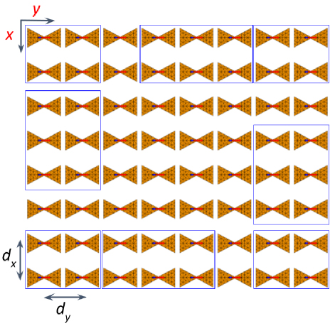
Figure 1: Periodic array of bow-tie antenna elements (see [9, Fig. 1]) with a spacing of at the excitation frequency of GHz. The subarray problems used to calculate the CBFs for the highlighted edge and corner elements are enclosed within rectangles.
The efficacy of the proposed CBFM algorithm is evaluated numerically by assessing its accuracy and computational cost in comparison to FEKO’s MoM solver and the domain Green’s Function method (DGFM) [91], as presented in section II part C.5.. The DGFM is selected for this comparison as a reduced-order solution technique with a (computational) cost-to-performance ratio similar to that of the CBFM, as detailed in [91]. Moreover, its commercial availability within FEKO has led to its extensive use in the analysis of large-scale antenna arrays across various applications, making it a suitable reference for comparison. To assess the accuracy of our algorithm, we focus on the prediction of both far-field and near-field characteristics, which are typically of interest to array designers, while also evaluating the accuracy of surface current distributions, which provide additional theoretical insights. To quantify the error in the approximation of the solution current for the th subdomain relative to FEKO’s reference MoM-based solution of (1), we define the norm-based relative error percentage for the th subdomain as follows:
| (8) |
where and represent the approximation of the solution and FEKO’s reference MoM-based solution vector for the th subdomain, respectively. Additionally, denotes the -norm. In the CBFM algorithm, the subdomain solution is approximated through the CBF expansion in (2).
To ensure an unbiased comparison, both the CBFM and DGFM algorithms were implemented in Julia, a high-performance programming language optimized for scientific computing [92]. The latter algorithm is implemented according to [91]. Additionally, to eliminate any potential impact of differing parallelization paradigms used in FEKO’s MoM solver and our Julia-based algorithmic implementations on the runtime of the studied solution methods, all algorithms were executed in a strictly serial manner. Furthermore, all simulations were conducted on an Intel i7-9700K processor running at 3.6 GHz with 32 GB of RAM.
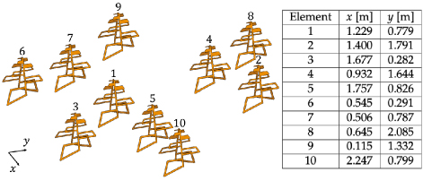
Figure 2: The irregular sparse array of 10 log-periodic antenna elements (see [9, Fig. 7]), excited at the frequency of GHz, with annotated indices and positions.
5. Numerical results
Before evaluating the accuracy of the CBFM algorithm, we first investigate the efficacy of the solution of a unit-cell element in an infinite, doubly periodic array environment. This infinite-array solution approximation is often used for the rapid estimation of the characteristics of large, truncated-periodic antenna arrays. While the accuracy of this approximation generally improves with increasing array size, its overall reliability remains inherently limited, as it does not rigorously account for MC and truncation effects within a finite array. This is demonstrated in Table 1, which shows the norm-based relative error percentage of the infinite-array solution approximation, calculated for each element of the bow-tie array problem shown in Fig. 1. As expected, the infinite-array solution approach predicts the solution for interior elements with reasonable accuracy; however, its performance progressively degrades toward the edges and corners of the array. At this stage, the CBFM algorithm is introduced, where the infinite-array solution is uniformly assigned as the CBF to each array element. These CBFs are then weighted with their corresponding coefficients obtained by solving the CBFM-based reduced-order matrix equation (3), which significantly improves the accuracy of the infinite-array solution approximation, as demonstrated in Table 2. This improvement can be attributed to the rigorous inclusion of the array MC effects during the construction of the reduced-order matrix system through (4).
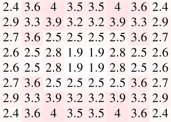
Table 1: Norm-based relative error percentage (8), considering the infinite-array solution approximation and MoM-based solution vectors for the elements of the bow-tie antenna array shown in Fig. 1
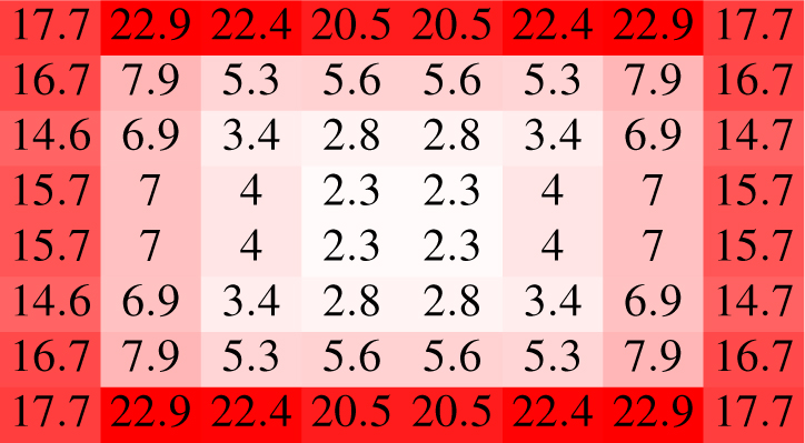
Nevertheless, in spite of this overall improvement, the error in the final solution remains higher for edge and corner elements in comparison to the interior elements. Note that, when using a single CBF per element, the spatial distributions (profiles) of the element’s CBF and its associated final solution are essentially identical, with the difference arising from the applied scaling by a complex weighting coefficient calculated in the presence of array MC effects. Therefore, the inclusion of MC effects via the weighting coefficient only partially counterbalances the error introduced by finite array truncation effects—which cause the largest perturbation in the solution from the assumed infinite-array solution approximation, and consequently the largest error—for edge and corner elements. To improve the solution accuracy while maintaining a single CBF per element, we employ a hybrid CBF generation strategy, in which the CBFs for edge and corner elements are extracted from the solutions of their respective subarray problems, while the interior elements retain the infinite-array solution as their CBF, as detailed in section II part C.3.. The improvement in accuracy in the final CBFM-based solution for edge and corner elements is evident from the error results presented in Table 3. To enable visual comparison of the errors presented in Tables 1 through 3, an identical color scheme has been applied across these tables, mapping the range between the minimum and maximum error values to their corresponding color codes.
Table 2: Norm-based relative error percentage (8), considering the CBFM-based and MoM-based solution vectors for the elements of the bow-tie antenna array shown in Fig. 1. In the CBFM algorithm, each array element is assigned an identical CBF corresponding to the infinite-array solution approximation
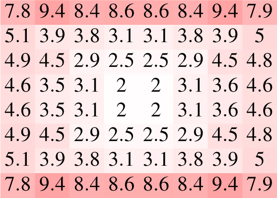
Table 3: Norm-based relative error percentage (8), considering the CBFM-based and MoM-based solution vectors for the elements of the bow-tie antenna array shown in Fig. 1. In the CBFM algorithm, an identical CBF corresponding to the infinite-array solution approximation is assigned to the interior elements, while the CBFs for the edge and corner elements are calculated by solving localized MoM-based subarray problems specific to theseelements
To assess the performance of the CBFM algorithm with a single CBF per element in relation to the applied CBF generation scheme for the truncated-periodic bow-tie antenna array problem, we compare its near-field and far-field results against FEKO’s reference MoM-based solutions. Specifically, we compare the electric near-field results in the observation plane of interest, as shown in Fig. 3, and the far-field (directivity) results in the elevation plane at , as shown in Fig. 4. These results suggest that although the CBFs for edge and corner elements more accurately represent the actual current distribution when a modified CBF generation scheme is used for these elements, the overall impact of this improvement on the accuracy of near- or far-field calculations may be limited in various practical scenarios [3]. Moreover, in many practical applications where the primary focus is on efficiently characterizing antenna array far-field patterns, both versions of the CBFM algorithm might produce similar design outcomes [3]. Nevertheless, the improved solution accuracy for the edge and corner elements, as shown in Table 3, suggests that for observation points closer to the antenna surface, the salutary effects of this improvement will be more noticeable. Finally, the limited accuracy of far-field results based on the infinite-array solution approximation, as displayed in Fig. 4, highlights the importance of integrating the CBFM into the solution algorithm to improve the accuracy in both near- and far-field predictions [3], leading to well-informed design decisions.
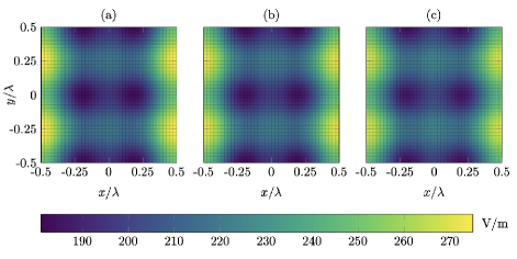
Figure 3: Surface plots illustrating the -component of the electric near field in the observation plane at , radiated by the uniformly excited bow-tie antenna array shown in Fig. 1, and calculated using: (a) the CBFM solver with an identical CBF corresponding to the infinite-array solution approximation for all array elements [2]; (b) the CBFM solver with an identical CBF for the interior elements and region-specific CBFs for the edge and corner elements [3]; and (c) FEKO’s MoM solver.
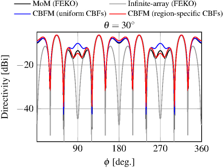
Figure 4: Directivity plots for the antenna array shown in Fig. 1.
Table 4: Norm-based relative error percentage (8), considering the top-level CBF and final solution vectors of the two-level CBFM algorithm and MoM-based reference solution vectors for the elements of the irregular sparse array of log-periodic antenna elements shown in Fig. 2. The third column shows the error associated with the th element’s CBF, calculated from its corresponding subarray problem of size (second column), given the RoI of corresponding to the excitation frequency of , while the last column presents the error associated with the final solution of this algorithm
| Element | CBF Error (%) | CBFM Solution Error (%) | |
| 1 | 4 | 6.1 | 6.6 |
| 2 | 2 | 8.5 | 7.4 |
| 3 | 3 | 3.1 | 3.3 |
| 4 | 3 | 6.9 | 5.1 |
| 5 | 4 | 5.9 | 6.7 |
| 6 | 2 | 7.5 | 5.2 |
| 7 | 4 | 6.3 | 5.0 |
| 8 | 2 | 8.0 | 6.1 |
| 9 | 2 | 2.9 | 2.5 |
| 10 | 2 | 4.0 | 2.9 |
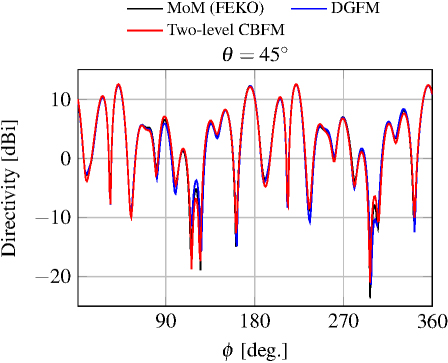
Figure 5: Directivity plots for the antenna array shown in Fig. 2.
For the analysis of the ISA of log-periodic antenna elements shown in Fig. 2, the RoI is set to relative to the excitation frequency. Consequently, each subarray defined by this RoI contains between 2 and 4 elements, as summarized in Table 4. In addition, Table 4 compares the norm-based relative error percentage for the CBFs derived from localized subarray-based CBFM formulations and the corresponding final solutions of the two-level CBFM algorithm, demonstrating relatively good accuracy of both representations when compared to the reference MoM-based solution. These results support the hypothesis that, in the two-level CBFM solution process, the shape of the solution for each element can be well approximated during the CBF generation step at the bottom level of this algorithm by considering only the MC interactions within the localized subarray problem associated with that element; while the contributions of elements outside the subarray are effectively accounted for by refining the generated CBFs at the top level using CBFM-based weighting coefficients. The effectiveness of the CBFM algorithm in modeling surface currents translates directly to accurate far-field characterization, as shown in Fig. 5, which compares the directivity results in the cut plane obtained using our method with the reference results from the DGFM and FEKO’s MoM-based solver. The CBFM-based result successfully reproduces the reference complex oscillatory directivity pattern, despite the approximations used in this algorithm [4].
Table 5 presents the computational costs and solution accuracy of the proposed two-level CBFM approach in comparison to DGFM-based and MoM-based reference solutions considering the studied ISA of log-periodic antenna elements. In addition, Table 6 provides an overview of runtime complexities of these solution methods at different stages of the solution process. The computational complexities listed in Table 6 were approximated by considering the total number of scalar multiplications of the most computationally intensive process in each step of the solution process, as detailed in [9].
Table 5: Computational costs and solution accuracy relative to FEKO’s MoM-based reference for different solver implementations, considering the 10-element ISA of log-periodic antenna elements shown in Fig. 2 with the RoI relative to the excitation frequency. The second column lists all unique DoFs encountered throughout the solution process, corresponding to the size of the matrix (or matrices) solved using a direct solution method (LU decomposition). For the two-level CBFM with local CBFM formulations, the listed DoFs correspond to: the size of the isolated element matrix, which is decomposed once and then reused to generate the primary and secondary CBFs at the bottom level; the maximum size of the reduced-order matrix across all subarray problems; and the size of the top-level reduced-order matrix, respectively. Runtime values in parentheses indicate the breakdown of the total runtime into the bottom-level CBF generation and the top-level CBFM solution processes. The peak memory requirement is calculated by assuming a double-precision storage scheme, with each complex matrix element stored using 16 bytes of memory
| # DoFs | Runtime (s) | Peak Memory | Usage (GB) | Error (%) | |||
| CBFM (local MoM) | 17040 | 10 | 838 | (825+13) | 4.33 | 5 | |
| CBFM (local CBFM) | 4260 | 16 | 10 | 96 | (83+13) | 0.27 | 5.21 |
| DGFM | 4260 | 65 | 0.27 | 6.33 | |||
| MoM (FEKO) | 42600 | 2719 | 27.04 | n/a |
Table 6: Overview of approximated runtime complexities for different solver implementations. Here, the symbol “” denotes the number of instances of different processes, while represents their corresponding computational complexity. The variables are defined as follows: is the number of subdomains; is the average subarray size; and represent the sizes of the MoM-based subdomain and array matrices, respectively. In the bottom-level CBFM algorithm, we assign a single primary CBF and a set of secondary CBFs to each subarray element, while retaining all CBFs following their orthogonalization via the SVD algorithm. Consequently, the total average number of CBFs per subarray element corresponds to the average subarray size . In deriving the runtime of generating the secondary CBFs, we use the following approximation: . Furthermore, assuming that , as is typically the case for geometrically large and complex antenna elements, the runtime complexity of the classical Golub-Reinsch SVD algorithm applied to the CBFs of each subarray element can be approximated as (see [94, Fig. 8.6.1]). In addition, note that for arrays composed of identical antenna elements, the generation of primary CBFs in the proposed CBFM algorithm requires only a single instance, as the base element matrix needs to be solved only once
| MoM | DGFM [91] | Proposed Two-Level CBFM Algorithm | ||||||
| # | # | |||||||
| MoM Matrix Generation | 1 | 1 | ||||||
| Generation of Primary CBFs | n/a | n/a | n/a | |||||
| Generation of Secondary CBFs | n/a | n/a | n/a | |||||
| SVD Ortho-gonalization | n/a | n/a | n/a | |||||
| Bottom-Level | CBFM | Systems Setup | n/a | n/a | n/a | |||
| Bottom-Level | CBFM | Systems | Solution | n/a | n/a | n/a | ||
| Top-Level | CBFM | System Setup | n/a | n/a | n/a | 1 | ||
| Top-Level | CBFM | System | Solution | n/a | n/a | n/a | 1 | |
| DGFM | Solution | n/a | n/a | n/a | ||||
| MoM Matrix | Solution | n/a | n/a | n/a | n/a | |||
Several observations can be made based on the results displayed in Table 5: (a) the proposed two-level CBFM approach, leveraging local CBFM formulations, greatly outperforms FEKO’s MoM-based reference solver in both runtime and peak memory consumption, achieving an order-of-magnitude improvement in both metrics while maintaining comparable accuracy in the solution current; (b) replacing CBFM-based local formulations with their MoM-based counterparts significantly increases the overall runtime, without providing substantial improvements in solution accuracy. However, the latter approach still considerably outperforms FEKO’s MoM solver in both the runtime and memory usage; (c) compared to the DGFM, our proposed approach achieves slightly improved accuracy, albeit with a slightly larger but competitive runtime. This overhead is likely due to the fact that neither algorithm is fully numerically optimized in Julia. However, the DGFM follows a more straightforward algorithmic implementation routine, potentially leading to faster execution times in the unoptimized implementations of these algorithms. More importantly, the runtime comparison does not fully reflect the theoretical advantages of our CBFM method in terms of numerical efficiency for many practical antenna array problems, as evidenced in Table 6. A key disadvantage of the DGFM in this context is its reliance on solving the active impedance matrix for each element independently using a direct solution method. The cumulative computational cost of this process is typically higher than that of dealing with the reduced-order systems at both levels of our CBFM algorithm. Note that in our method, the runtime is typically dominated by the construction of the reduced-order systems, while the additional solution overhead is often negligible for many practical array problems, as is evident from Table 5. In addition, a key advantage of our approach over the DGFM is its ability to systematically enhance solution accuracy. This can be achieved by increasing the RoI to define larger subarray problems or by incorporating higher-order CBFs at the bottom level to more effectively capture interelement coupling effects, leading to improved solution fidelity, whereas the standard DGFM formulation lacks this flexibility.
Note that the size of the studied array example is not constrained by the computational complexity of our method, which significantly improves upon those of MoM- and DGFM-based solvers, as demonstrated in Tables 5 and 6. Instead, the maximal array size is limited by the use of FEKO’s full-rank array matrix, which exceeds the RAM capacity of standard desktop machines even for moderately sized log-periodic antenna arrays. Meanwhile, the numerical efficiency of our proposed two-level CBFM algorithm suggests that significantly larger arrays can be analyzed using our method, even on standard machines, such as the ISA composed of log-periodic antenna elements shown in [45, Fig. 5]. However, achieving this would require applying a matrix compression scheme, such as the adaptive cross approximation (ACA) algorithm [93], to significantly reduce the effective size of the moment matrix. This could be implemented in two ways: first, by precalculating and storing the compressed moment matrix for the entire antenna array at the initial step of the two-level CBFM algorithm, allowing its submatrices to be reused throughout different stages of this algorithm; or alternatively, by dynamically recalculating the intra- or interelement coupling submatrices on demand, rather than storing them in advance. This represents a trade-off between runtime and memory consumption, where the first approach minimizes runtime by avoiding repeated calculations of the coupling submatrices at the cost of increased memory consumption. In contrast, the second approach reduces the memory usage by storing only small-sized compressed submatrices instead of the full array matrix, enabling the simulation of larger arrays on machines with fixed RAM capacity, albeit at the expense of increased runtime due to repeated calculations of the same submatrices. Nevertheless, when using the first approach and excluding matrix generation times from the analysis—since this matrix is required for all methods considered—the complexities listed in Table 6 suggest that for elements with a larger number of DoFs per element and larger array sizes, the runtime advantages of our method become more pronounced due to its favorable scaling. Finally, the proposed two-level CBFM approach is fully parallelizable, allowing for its numerically efficient implementation on multi-threaded CPUs and GPUs.
6. Future work and concluding remarks
As part of the future work, in addition to applying the matrix compression scheme to further reduce the computational requirements of the proposed two-level CBFM formulation, we will extend the analysis of this method to antenna arrays above an infinite ground plane. Since the impact of the ground plane is embedded into the calculation of the full or compressed array moment matrix, the proposed method can be applied in its present form. In addition, we will investigate the potential integration of the overlapping subarray strategy detailed in [75] into our algorithm to efficiently account for the coupling effects from array elements just outside the specified RoI. This would enhance the accuracy of the single-CBF representation for each element in the CBFM algorithm. The use of an overlapping subarray strategy to generate subarray CBFs with improved accuracy—or alternatively, a different approach, such as employing higher-order CBFs beyond secondary—may be particularly important when analyzing array problems with connected subdomains, where the current CBF generation scheme may not effectively capture strong MC effects between subdomains. Furthermore, to extend the applicability of this method to printed antenna array problems on multilayered substrates, we will investigate its integration with the equivalent medium approach (EMA), as detailed in section II part D., or alternatively, by embedding substrate effects directly during the construction of the MoM matrix. The former approach seamlessly integrates into our method with negligible computational overhead but may not fully capture exact field interactions across layers, surface wave modes, or material inhomogeneities, particularly in antenna arrays with relatively thick substrates. Conversely, the explicit use of a multilayered Green’s Function generally improves accuracy; however, this improvement comes at the expense of significantly increased computational cost, an effect that becomes particularly pronounced at millimeter-wave frequencies, such as in 5G/6G system applications, as detailed in section II part D.. Moreover, an iterative formulation of this algorithm, inspired by [9], will be explored to improve solution accuracy in applications with high-precision requirements.
In this section, we presented a novel two-level formulation of the CBFM algorithm for efficient analysis of large-scale antenna arrays. In this approach, local CBFM formulations generate a single CBF per element at the top level. Our results demonstrate that this method achieves over an order-of-magnitude improvement in both memory efficiency and runtime compared to MoM. Furthermore, it ensures reliable accuracy not only in the antenna far field—typically the primary concern for array designers—but also in the near field, establishing the proposed two-level CBFM algorithm as a powerful and highly efficient alternative for analyzing large, complex antenna arrays.
D. Toward a numerically efficient CBFM implementation for mm-wave problems
While the previous section focused on the CBFM with a single basis per element and outlined future research directions within that framework, a broader paradigm shift is necessary to enhance the effectiveness of the general CBFM framework in addressing the challenges of modern antenna analysis and design. One of the primary challenges today is the growing demand for efficient electromagnetic simulations at millimeter-wave (mm-wave) frequencies and beyond, particularly in the context of 5G/6G communication systems, as discussed in section II of [1]. The shift to higher operating frequencies, coupled with fixed space constraints in electronic devices, has significantly increased the electrical sizes of antennas and circuit modules, introducing new challenges for their effective EM simulation in the mm-wave region. A major challenge in this context concerns the numerically efficient calculation of Green’s Functions, which are essential for MoM-based analysis of antennas and circuits printed on layered media [95]. Herein, the Sommerfeld integrals used in the calculation of Green’s functions can become highly oscillatory and slowly decaying, reducing solution accuracy while increasing the runtime [95].
In section II of [1], an efficient numerical strategy for evaluating the Sommerfeld integrals in layered media problems is discussed, as recently proposed in [95]. This approach employs a strategic interpolation and extrapolation scheme to minimize the number of sample points needed to accurately represent the integrand, enabling analytical integration which in turn significantly accelerates the calculation of Green’s functions [95]. In contrast, section III of [1] presents a novel strategy for the numerical modeling of planar circuits and antennas printed on layered media, which completely eliminates the need for constructing the layered-medium Green’s Function in the MoM. This strategy utilizes the EMA to replace the original layered geometries with equivalent geometries embedded in an infinite homogeneous medium, characterized by the corresponding effective dielectric constant. By replacing the original geometry with the equivalent one, the problem that originally required using a volumetric MoM formulation can instead be effectively addressed using a surface formulation based on Green’s Function in a homogeneous medium, significantly improving the computational efficiency of the solution process.
In addition to its integration with the EMA, we highlight a promising research direction for improving the numerical efficiency of the CBFM algorithm by formulating it based on quadrilateral surface discretization (see [96, Fig. 3]) with piecewise sinusoidal (PS) basis functions between pairs of quadrilateral elements, as in [28], instead of using conventional triangular meshing with RWG basis functions. The three key benefits of using quadrilateral discretization with PS basis functions are: (a) the reduced number of basis functions compared to the number of RWG basis functions for identical patch and mesh sizes, combined with the more favorable scaling with domain size, as demonstrated in Fig. 6; (b) the ability to efficiently generate matrix elements by testing observation basis functions against the scattered fields from sinusoidal current filaments or sheets corresponding to source basis functions, which are available in closed form (see [28] and references therein). This eliminates the need for evaluating computationally intensive numerical integrals when generating these elements in conventional MoM algorithms that use triangular discretization with RWG basis functions; and (c) the ability to reuse previously calculated matrix elements for equivalent pairs of basis functions, leveraging the inherent geometric regularity and repeatability of the structured mesh. Note that quadrilateral and triangular meshes can be hybridized to model arbitrary planar geometries, such as the bow-tie antenna array shown in Fig. 1, with the former used in interior regions and the latter conforming to the geometry’s edges.
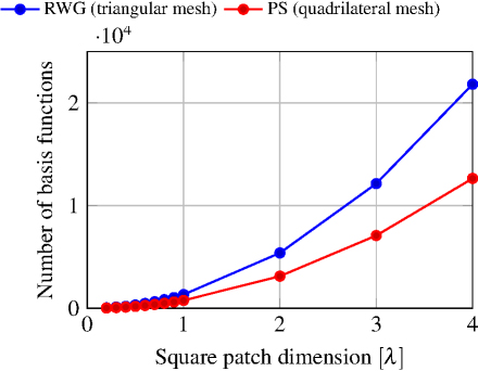
Figure 6: Comparison of the number of RWG basis functions for triangular discretization in FEKO versus the number of PS basis functions for quadrilateral discretization of a square patch with varying dimensions, using a mesh size.
To fully leverage the computational advantages of quadrilateral mesh discretization with PS basis functions, the EMA, and the CBFM, a hybrid approach is being developed in our group that integrates these methods. This approach utilizes the EMA to eliminate the direct computation of Green’s Functions for antenna arrays printed on layered media, the quadrilateral MoM with PS basis functions to efficiently generate the array moment matrix, and the CBFM to accelerate the solution process. Initial results from this study will be presented in future work.
III. LCPML-LOG: A PARAMETER-FREE PERFECTLY MATCHED LAYER METHOD FOR FINITE METHODS
In this section, we introduce the LCPML-log method, an advanced Locally-Conformal Perfectly Matched Layer (LCPML) technique optimized for addressing mesh truncation challenges in solving electromagnetic radiation and scattering problems using the FEM. LCPML-log is distinguished by (a) achieving optimal PML performance without requiring parameter tuning and (b) yielding superior results even with a minimal, single-layer PML configuration. This approach represents a significant advancement in both cost-effectiveness and robustness in PML technology.
In computational electromagnetics, the PML is essential for simulating open-region electromagnetic wave problems, providing an artificial boundary that absorbs outgoing waves with minimal reflection. Traditional PML approaches, developed in the 1990s, laid the foundation for this technology but often struggle with arbitrary geometries and require complex parameter adjustments [97, 98, 99, 100, 101, 102]. The Locally-Conformal PML, introduced by Ozgun and Kuzuoglu in 2007 [103], [104], revolutionized the field by offering a more flexible, geometry-agnostic solution.
Recently, Ozgun and Kuzuoglu have developed a variant of the LCPML method, named LCPML-log, which utilizes a logarithmic decay function in its coordinate transformation [105, 106]. Unlike its predecessor, LCPML-log modifies the matrix formation phase of the FEM, embedding the logarithmic function directly into the core of the computational process, rather than simply substituting real coordinates with complex ones. While this method may require a more intricate implementation, it offers clear benefits: enhanced performance without the need for prior parameter adjustments and increased accuracy with a single PML layer. This efficiency leads to a significant reduction in computational resources, making LCPML-log a breakthrough for large-scale simulations.
Initially developed for 2D electromagnetic problems governed by the scalar Helmholtz equation [105], LCPML-log was subsequently extended to address 3D problems involving the vector wave equation [106]. This section provides a brief overview of the LCPML-log method, supplemented with examples that demonstrate its effectiveness and practicality.
A. Mathematical formulation
The LCPML-log method constructs a PML region that conforms to an arbitrary region (), designed to enclose the sources or objects of interest within the smallest possible convex set. As shown in Fig. 7, the PML region is defined by its inner and outer boundaries ( and ). Each point in the PML region is mapped to a complex coordinate through the following transformation, assuming time-harmonic fields of the form :
| (9) |
where is the decay or attenuation function, which is a monotonically increasing function of the decay parameter confined within . The unit vector indicates the direction of decrease within the PML region. The position vectors , , and correspond to points within , , and , respectively, while denotes the wavenumber, and the Euclidean norm is used for magnitude calculations. The most critical component in this transformation is the decay function , which drives the transformation and is defined as follows:
| (10) |
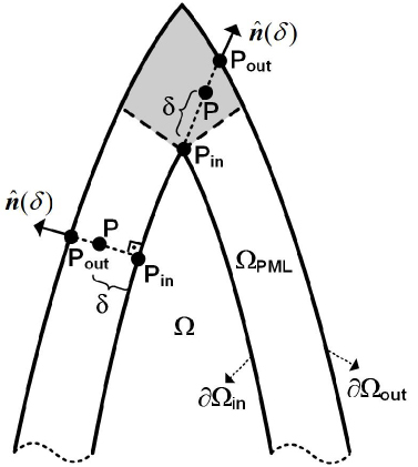
Figure 7: Illustration of the LCPML-log method.
In developing the FEM formulation, we start by deriving the weak variational form of the wave equation via the weighted residual method. The computational domain is then discretized into a mesh of elements—triangular in 2D and tetrahedral in 3D—over which the weak form is solved. The integration necessary for the weak form is simplified by mapping the original domain to a master element (), using isoparametric mapping. The coordinates within this master element are expressed using the same shape functions as those for the unknown field variables, facilitated by a Jacobian matrix.
LCPML-log’s uniqueness lies in its handling of the Jacobian matrix. The process involves two successive transformations: . The complex coordinates, now composite functions, are mapped through these stages, i.e., . Here, for example, is expressed as a combination of the shape functions and real coordinates: , where is the real coordinate of the -th node, is the -th shape function, and is the number of nodes in an element. Here, represents the Jacobian matrix, where pertains to the standard FEM transformation and captures the logarithmic transformation unique to LCPML-log.
The entries of are given in (11), where , , and represent the directional components of the unit vector . Partial derivatives such as are computed analytically, when possible, or numerically by using the functional dependence of boundary points. For numerical computation, central differencing formulas can be applied. The boundary points on the PML boundaries are determined by employing the Lagrange multiplier method, as detailed in [105] and [106].
| (11) |
B. Numerical results
To demonstrate the performance of the LCPML-log method, we first consider the problem of constructing the free-space Green’s Function for the Helmholtz equation within a given domain. Specifically, we examine a scenario where a line source located at (0.2 m, 0) radiates within a circular region of radius m, as depicted in Fig. 8. The mean-square error (MSE), which compares the computed and analytical field values, is plotted as a function of the number of PML layers for different wavelength () values. We observe that the LCPML-log method outperforms the original LCPML method, particularly when using a single PML layer. As evident from the vertical axis (MSE values), even with a single layer, the LCPML-log method achieves significantly low error levels across different frequencies and mesh resolutions. This indicates that increasing the number of PML layers beyond a certain point does not necessarily provide a substantial accuracy improvement, as the error is already minimized at very low levels. Moreover, many applications require broadband frequency sweeps using the same mesh, which poses challenges in both computational cost and accuracy. The LCPML-log method, as demonstrated by the almost flat nature of the error curves, remains robust and nearly independent of frequency even with a relatively coarse mesh. This stability further supports the argument that a large number of PML layers is not essential, as the method maintains low error levels across a wide frequency range with minimal computational effort.
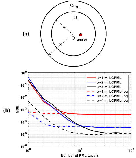
Figure 8: A line source radiating in a circular PML region. (a) Geometry, (b) plot of mean-square error (MSE) vs. number of PML layers. (Axes are logarithmic.)
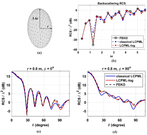
Figure 9: Golden ellipsoidal PML. (a) Geometry, (b) backscattering RCS, (c) bistatic RCS profile at plane, (d) bistatic RCS profile at plane.
Next, we examine a scattering problem involving a conducting ‘golden’ ellipsoid, where the ratio of the semi-major axis to the semi-minor axis is approximately the golden ratio (i.e., 1.6) (see Fig. 9). The object is illuminated by an -polarized plane wave propagating along the -axis, with a conformal PML applied around its spherical boundary. The wavenumber is , corresponding to a wavelength of 1 m. The computational setup includes a cell size of and a separation of between the inner PML boundary and the object. A single PML layer with a thickness of is employed. The radar cross-section (RCS) values obtained using the LCPML method, optimized for best performance, are compared in Fig. 9 with those from the LCPML-log method, which requires no parameter tuning. The results are also compared with those obtained using the commercial electromagnetic solver FEKO. The results clearly demonstrate that LCPML-log performs well even with a single PML layer and without the need for parameter adjustments.
IV. GPU ACCELERATION OF MOM AND FDTD
In this section, we briefly discuss the GPU acceleration of MoM and, separately, the FDTD algorithm. GPU Acceleration of CEM codes [107] is currently a very popular topic, and we have included brief writeups in this work for the sake of completeness. For additional details, the reader is encouraged to refer to select publications on this topic that have been cited herein.
The Graphics Processing Unit (GPU) is a highly parallelized stream processor, originally designed for image processing, where it executes parallel operations on all pixels simultaneously. Consequently, GPUs are optimized for handling large-scale data that is uniform in type and exhibits minimal interdependency. Due to differing design objectives, the architecture of GPUs significantly contrasts with that of Central Processing Units (CPUs). As illustrated in Fig. 12, the CPU architecture comprises key components such as a controller (which orchestrates the operation of various units), an arithmetic logic unit (which performs data processing), registers, cache, and data/control/status buses. The CPU’s functions include program control (regulating the order of instruction execution), operation control (managing the execution of instructions), timing control (coordinating the timing of operations), and data processing (performing arithmetic and logical calculations). In essence, the CPU manages the temporal and spatial control of instruction and data flow. It is particularly adept at handling complex operations like distributed tasks and coordinated control, making it highly versatile.
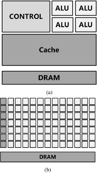
Figure 10: Comparison between GPU and CPU architectures
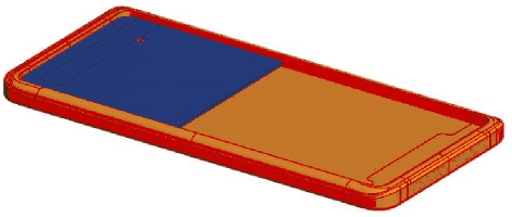
Figure 11: Cellphone model
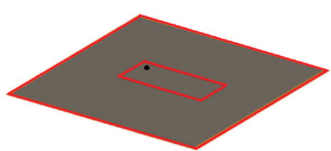
Figure 12: Comparison between GPU and CPU architectures
In contrast, GPUs consist of numerous processing units and feature long pipelines, but the design of their logical units is relatively simple. The number of cores in a GPU far exceeds that of a CPU, allowing the same instruction to be dispatched to multiple cores to process different data simultaneously. This architecture makes GPUs particularly well-suited for tackling computationally intensive tasks.
General-purpose computing on GPUs (GPGPU) refers to using graphics cards for general-purpose computations beyond rendering graphics. In recent years, the computational speed of GPU units has increased dramatically and, in some applications, GPUs have significantly outperformed CPUs. This has led to the emergence of a new research field: GPGPU, which focuses on utilizing GPUs for a broader range of computational tasks beyond traditional graphics processing.
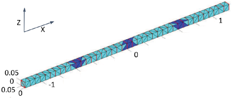
Figure 13: Cellphone model.
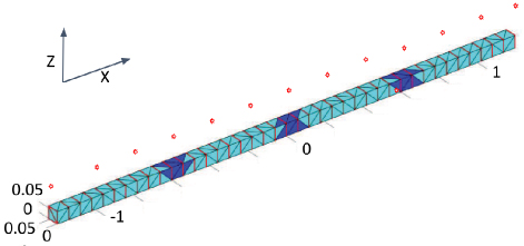
Figure 14: Simplified full-size cellphone.
A. GPU acceleration of MoM
Operation of 5G mobile devices at millimeter-wave frequencies (e.g., 30 GHz) introduces substantial complexity, leading to significantly increased problem sizes compared to sub-5 GHz operation. This imposes a significant computational burden, since it demands extensive CPU time and memory resources for electromagnetic analysis. To effectively mitigate these challenges, we propose and implement several acceleration techniques: geometry simplification, numerical reduction of degrees of freedom, and GPU-based parallel processing. Primary memory reduction is achieved via the CBFM, an efficient iteration-free technique for compressing basis functions [7]. CBFM has been extensively applied and investigated, including for the analysis of structures embedded in multilayered media [108].
These acceleration techniques are illustrated by using the geometry of a mobile device, comprising a metallic frame and an antenna mounted on a layered substrate (see Figs. 13 and 14). The initial step involves geometrical simplification without compromising the device’s electrical characteristics. This measure yields a significant reduction in the number of degrees of freedom, from 99738 down to 1892 unknowns at 30 GHz. Subsequently, the CBFM formulation, originally developed for scattering analysis, is adapted for layered media antenna applications by employing two distinct types of excitations—Edge Port(EP) and Dipole Moment (DM)—to generate the CBFs for the antenna structure [109]. Compared to conventional MoM, CBFM inherently reduces the dimension of the system matrix. This reduction is achieved irrespective of the excitation type, and our study indicates that the performance of the EP excitation is superior. This is because EP and DM excitations incorporate near-field components, including content related to the ‘invisible’ spectrum (evanescent waves) that are typically absent in traditional plane wave excitations, and this, in turn, enhances the accuracy of the representation. The impedance matrix, , computed via MoM, is utilized to construct the CBFs. GPU acceleration significantly expedites this process by parallelizing the computationally intensive filling of the MoM matrix. The MoM mesh and geometrical data are initially transferred to GPU global memory. The rows of the MoM impedance matrix are then computed in serial batches. Within each batch, the matrix elements are calculated in parallel on the GPU, with each element computation assigned to a dedicated GPU thread. Upon completion of a batch computation, the elements are copied back from the GPU global memory to CPU host memory for subsequent use in solving the MoM linear system. To mitigate the overhead associated with GPU-CPU data transfer initialization, a large GPU batch size is selected to maximize the utilization of the global memory. Numerical results confirm that leveraging GPU parallel processing substantially reduces fill time of the MoM matrix.
Future development of the GPU-accelerated CBFM scheme will involve defining GPU batches based on the MoM interactions required for generating a set of CBFs, rather than simply grouping a fixed number of MoM matrix rows. Following GPU processing of a batch, the MoM elements relevant to CBF construction will be copied back to the CPU host, where the SVD for forming the CBFs will be performed.
1. CBFM for microwave circuit and antenna problems
Based on the mixed-potential integral equation (MPIE), CBFs are constructed by using a set of low-level basis functions, specifically the Rao-Wilton-Glisson (RWG) functions. For each CBF level , the corresponding reduced matrix equation is formulated as:
| (12) |
To effectively adapt CBFM for millimeter-wave circuit and antenna problems, we utilize EPs defined on the surface of the analyzed structure (see Fig. 15). This approach is the natural choice for constructing the excitation vector in antenna problems, providing a direct interface to circuit ports, in contrast to plane wave excitations used in scattering analysis. As an illustrative example, the dipole geometry is partitioned into four blocks; the dark blue faces in the figure delineate the extended region used in the CBFM construction, while the red lines indicate the EPs oriented along the x-axis. Furthermore, in an antenna application employing a single delta-gap source for excitation, this source—implemented as an EP—must be included as one of the contributions to the excitation vector.
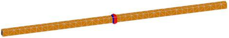
Figure 15: Edge ports on a dipole.
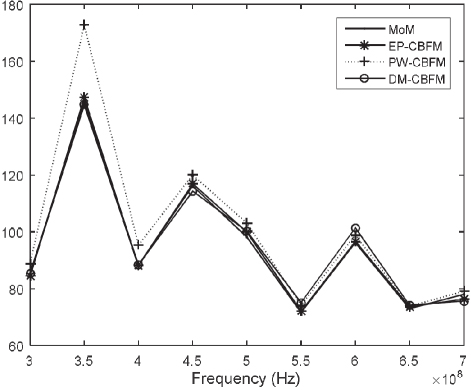
Figure 16: Dipole moments above a dipole.
An alternative excitation strategy employs sources that are neither solely far-field (e.g., a plane wave) nor located exclusively on the object’s body (e.g., an EP, as illustrated in Fig. 16). In this method, equivalent dipole moments positioned in the vicinity of the object are selected as sources to generate the excitation matrix. This inherently ensures the inclusion of both near-field (evanescent) and far-field (propagating) information, which is crucial for accurate CBF construction.
2. Numerical results
We now present some numerical results demonstrating the accuracy and efficiency of applying CBFM to antenna problems, along with the effectiveness of GPU acceleration. The first example analyzes a Perfect Electric Conductor (PEC) dipole in free space (see Fig. 17). For the CBFM implementation, the dipole geometry is partitioned into four blocks along its longitudinal axis, and a delta gap port is utilized for excitation at the center. The analysis is performed across a frequency range from 300 MHz to 700 MHz, with a step size of 50 MHz. The antenna structure is discretized by using 324 triangular elements, with element lengths approximately 0.1 wavelengths at 500 MHz. For constructing the CBFs, an extension region equivalent to 0.1 wavelengths at 500 MHz is employed. The computed input impedance () is plotted in Fig. 18, using results obtained from the conventional MoM as a reference for validation. Table 7 summarizes the SVD down-selection thresholds, as well as the number of samples and unknowns characterizing the reduced matrices for different excitation types: EP denotes edge-port, PW denotes plane-wave, and DM denotes dipole-moment excitation.
Figure 17: PEC dipole.
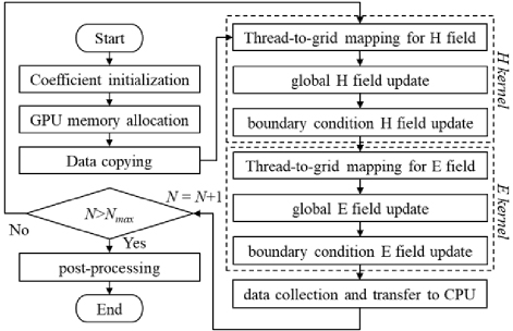
Figure 18: Z11 of example 13 obtained by using CBFM.
Table 7: Parameters and results of example 13
| Method | Threshold | Samples | Unknowns | |
| Min. | Max. | |||
| EP-CBFM | 0 | 96 | 96 | 96 |
| PW-CBFM | 1e-3 | 400 | 110 | 184 |
| DM-CBFM | 0 | 120 | 120 | 120 |
| MoM | 0 | 0 | 486 | 486 |
Our second numerical example analyzes a Perfect Electric Conductor (PEC) cross situated on the interface of a layered medium (see Fig. 19). This case is specifically employed to illustrate the computational acceleration achieved using GPU processing. The cross consists of arms measuring 10 wavelengths in length and 2 wavelengths in width. The layered medium is backed by a PEC plane. The analysis is conducted at 30 GHz, involving a total of 12085 unknowns. Table 8 presents the matrix fill-time, which clearly demonstrates significant computational acceleration when utilizing the GPU. The hardware platform used for this comparison included an Nvidia GTX860M GPU and an Intel I7-4710HQ CPU. The system was equipped with 8 GB of host memory. For comparative purposes, the CPU-based numerical results were obtained using commercial electromagnetic simulation software.
Figure 19: PEC cross embedded in layered medium.
Specifically, the GPU acceleration process [110, 111] is organized as follows:
All geometrical and material data required for MoM computations are first transferred to GPU global memory.
The impedance matrix is computed in batches of rows. Each batch is processed serially, while the elements within a batch are computed in parallel on the GPU. Each thread handles one matrix element (i.e., a source-observer pair).
After completing each batch, the results are copied back from GPU global memory to CPU memory. This approach is designed to balance GPU memory usage and data transfer overhead. To reduce the latency of memory transfers, the batch size is chosen to maximize the occupancy of GPU global memory.
The MoM impedance matrix computed in this way is subsequently used to form the reduced-order system in the CBFM framework.
In our current workflow, SVD is performed on the CPU after GPU-based computation of the MoM matrix elements.
Additional detail on GPU acceleration may be found in [112, 113, 114, 115, 116].
Table 8: Time used for matrix filling on different platforms
| Platform | Matrix filling time (minutes) |
| GPU | 0.7 |
| 1 CPU-Core | 26.6 |
| 2 CPU-Core | 20.0 |
| 4 CPU-Core | 24.0 |
| 6 CPU-Core | 26.4 |
| 8 CPU-Core | 26.5 |
B. GPU acceleration of FDTD
Since its inception, the FDTD method has developed into a mature and comprehensive numerical computation technique. Its straightforward and intuitive implementation, combined with its applicability to various computational models, has led to its widespread use and recognition as one of the fundamental methods in computational electromagnetics. However, due to the effects of numerical dispersion and stability, as well as the limitations of CPU floating-point performance, single-CPU implementations of the FDTD method can only handle the simulation and analysis of electrically small problems. These simulations may take several hours or even days to complete, and the simulation of electrically large targets presents even greater challenges. When applied to large-scale electromagnetic simulations, the FDTD method requires extensive memory and computing time.
To address these limitations, researchers have extensively explored several approaches, including higher-order FDTD methods, time-domain multiresolution analysis, and parallel FDTD algorithms. Among these, parallel FDTD, combining the computational power of parallel processing with the simplicity and clarity of the FDTD method, has gained prominence, particularly with the rapid advancement of GPGPU [117, 118, 119, 120].
Figure 20: Flowchart of the GPU-based parallel FDTD algorithm.
The workflow of the GPU-accelerated parallel FDTD algorithm is shown in Fig. 20. In this approach, the GPU acts as a coprocessor, working in tandem with the CPU. The program flow is divided into two parts: the host (CPU) part and the device (GPU) part, as depicted in Fig. 20. The right side of Fig. 20 represents the device section, which is executed by the GPU, while the left side shows the host section, managed by the CPU. The CPU primarily handles tasks such as memory allocation, field initialization, and time advancement of the simulation. The GPU is responsible for computationally intensive operations, performing field value calculations at each time step and updating the electric and magnetic fields in a recursive manner.
Using the component as an example, at each time step, the GPU reads the previous values, along with the and values, computational coefficients, and auxiliary variables related to boundary conditions from global memory. The GPU first executes the FDTD standard update equation kernel in parallel to compute the field values across the entire domain. After that, it runs a boundary condition kernel in parallel to update the field components located at the boundaries. Once this is complete, the new values and the associated auxiliary variables for the boundary conditions are written back to global memory for use in the field updates during the next time step.
The calculation process for other field components follows a similar procedure. After all field components for a given time step are computed, the CPU advances the simulation to the next time step, allowing the GPU to begin the next round of field calculations. The reason for using the CPU to handle time advancement is that Compute Unified Device Architecture (CUDA) lacks global thread synchronization capabilities, which is essential for FDTD’s time-domain iterations. The algorithm requires that all (or ) field components be fully computed at a given time step before advancing to the (or ) field components. To address this, the device-side computation is split into two kernel functions: one for computing the E fields and another for computing the H fields, which are executed sequentially. The CPU ensures global synchronization between these two steps, preventing computation errors that would result from improper synchronization.
In this work, parallel computation is implemented by assigning one thread to handle each Yee cell. For example, in the case of calculating the Ex component, within an FDTD computational domain of dimensions , the number of components to be updated is typically . Both the grid and block structures used in this paper are one-dimensional, with each block consisting of nT threads. The CUDA thread index corresponding to the component at position () in the FDTD domain can be calculated by:
| (13) |
| (14) |
where represents the floor operation, and % denotes the modulo operation. It is important to note that must be a multiple of the GPU’s warp size, which is typically 32. This thread allocation strategy ensures that the memory assigned to each block is contiguous in the x-direction, which satisfies global memory alignment requirements. This allows for continuous memory access, thereby improving the effective memory bandwidth.
The authors are currently pursuing further research in the area of GPU/FDTD acceleration and plan to report the results in a future publication [121].
In summary, GPUs have become indispensable for accelerating computational electromagnetics simulations. In FEM, GPUs enhance the solution of large sparse matrix systems through parallelized iterative solvers and efficient handling of element-wise computations. For MoM, which involves dense matrix operations for surface integral equations, GPUs leverage their high memory bandwidth and parallel processing capabilities to accelerate matrix filling and matrix-vector products, significantly reducing solution times. In FDTD, GPUs excel by parallelizing the explicit time-stepping updates across the computational grid, enabling real-time or large-scale simulations of wave propagation and scattering problems. By exploiting massive parallelism, GPUs deliver orders-of-magnitude speedups over CPUs, making them essential for high-performance electromagnetic analysis in research and industry. Future advancements in exascale computing, AI-driven numerics, and heterogeneous architectures will further push the limits of GPU-accelerated EM simulation.
V. CONCLUDING REMARKS
In this work, we have presented several innovative CEM techniques for numerical modeling of microwave circuits, antennas, and array configurations, with special emphasis on techniques for efficient simulation at millimeter-waves, and beyond, where the conventional simulation techniques become both memory-intensive and time-consuming. We have focused on solving a variety of practical design and analysis problems and have presented a wide array of example geometries that are useful for 5G/6G applications. Looking into the future, the authors are currently developing an AI-based antenna design software [122] which will integrate some of the simulation algorithms presented in this work to speed up the design process.
ACKNOWLEDGMENT
The authors acknowledge their team members and research collaborators, including Chao Li, Donia Ouesleti, Koushik Dutta, Yang Su, and others for their contributions and helpful discussions. We thank Dr. Danie Ludick for pointing us to the “cemagg/SUN-EM” GitHub library, which was used to parse FEKO’s MoM-based data into MATLAB. We also acknowledge the responsible use of ChatGPT, developed by OpenAI, for assistance in text editing during the preparation of this manuscript. The tool was used solely to improve clarity and language, without contributing to the scientific content of the paper.
REFERENCES
[1] R. Mittra, O. Ozgun, V. Kaim, A. Nasri, P. Chaudhary, and R. K. Arya, “Novel strategies for efficient computational electromagnetic (CEM) simulation of microstrip circuits, antennas, arrays and metamaterials Part-I: Introduction, layered medium Green’s Function, equivalent medium approach,” Applied Computational Electromagnetics Society (ACES) Journal, pp. 000-000, 2025.
[2] T. Marinović and R. Mittra, “Efficient analysis of large periodic array antennas using the characteristic basis function method,” in 2022 IEEE Int. Symp. Antennas Propag. USNC-URSI Radio Sci. Meeting, pp. 417-418, Denver, CO, USA, July 2022.
[3] T. Marinović and R. Mittra, ‘‘Characteristic basis function method using single high-level basis function per subdomain for efficient analysis of large periodic array antennas,” in 2023 IEEE Int. Symp. Antennas Propag. USNC-URSI Radio Sci. Meeting, pp. 807-808, Portland, OR, USA, July 2023.
[4] T. Marinović and R. Mittra, “Characteristic basis function method using single high-level subdomain basis function for efficient analysis of irregular sparse array antennas,” in 2024 IEEE Int. Symp. Antennas Propag. INC/USNC-URSI Radio Sci. Meeting, pp. 229-230, Florence, Italy, July 2024.
[5] S. Rao, D. Wilton, and A. Glisson, “Electromagnetic scattering by surfaces of arbitrary shape,” IEEE Trans. Antennas Propag., vol. 30, no. 3, pp. 409-418, 1982.
[6] F. Gustrau and D. Manteuffel, EM Modeling of Antennas and RF Components for Wireless Communication Systems. Berlin and Heidelberg: Springer-Verlag, 2006.
[7] V. V. S. Prakash and R. Mittra, ‘‘Characteristic basis function method: A new technique for efficient solution of method of moments matrix equations,” Microw. Opt. Technol. Lett., vol. 36, no. 2, pp. 95-100, Jan. 2003.
[8] R. Maaskant, Analysis of large antenna systems, Ph.D. thesis, Eindhoven University of Technology, Eindhoven, 2010.
[9] T. Marinović, R. Maaskant, R. Mittra, and G. A. E. Vandenbosch, “Comparison of CBFM-enhanced iterative methods for MoM-based finite antenna array analysis,” IEEE Trans. Antennas Propag., vol. 70, no. 5, pp. 3538-3548, May 2022.
[10] E. Lucente, G. Tiberi, A. Monorchio, G. Manara, and R. Mittra, “The characteristic basis function method (CBFM): A numerically efficient strategy for solving large electromagnetic scattering problems,” Turkish J. Electr. Eng., vol. 16, no. 1, pp. 41-56, 2008.
[11] E. Lucente, A. Monorchio, and R. Mittra, “An iteration-free MoM approach based on excitation independent characteristic basis functions for solving large multiscale electromagnetic scattering problems,” IEEE Trans. Antennas Propag., vol. 56, no. 4, pp. 999-1007, Apr. 2008.
[12] C. Delgado, R. Mittra, and F. Cátedra, “Accurate representation of the edge behavior of current when using PO-derived characteristic basis functions,” IEEE Antennas Wireless Propag. Lett., vol. 7, pp. 43-45, 2008.
[13] C. Delgado, M. F. Cátedra, and R. Mittra, “Application of the characteristic basis function method utilizing a class of basis and testing functions defined on NURBS patches,” IEEE Trans. Antennas Propag., vol. 56, no. 3, pp. 784-791, 2008.
[14] C. Delgado, M. F. Cátedra, and R. Mittra, “Efficient multilevel approach for the generation of characteristic basis functions for large scatters,” IEEE Trans. Antennas Propag., vol. 56, no. 7, pp. 2134-2137, 2008.
[15] C. Delgado, E. García, F. Cátedra, and R. Mittra, “Generation of characteristic basis functions defined over large surfaces by using a multilevel approach,” IEEE Trans. Antennas Propag., vol. 57, no. 4, pp. 1299-1301, 2009.
[16] J. Laviada, F. Las-Heras, M. R. Pino, and R. Mittra, “Solution of electrically large problems with multilevel characteristic basis functions,” IEEE Trans. Antennas Propag., vol. 57, no. 10, pp. 3189-3198, Oct. 2009.
[17] J. Laviada, J. Gutierrez-Meana, M. Pino, and F. Las-Heras, “Analysis of partial modifications on electrically large bodies via characteristic basis functions,” IEEE Antennas Wireless Propag. Lett., vol. 9, pp. 834-837, 2010.
[18] L. Hu, L.-W. Li, and R. Mittra, “Electromagnetic scattering by finite periodic arrays using the characteristic basis function and adaptive integral methods,” IEEE Trans. Antennas Propag., vol. 58, no. 9, pp. 3086-3090, 2010.
[19] J. Laviada, M. R. Pino, and F. Las-Heras, “Generation of excitation-independent characteristic basis functions for three-dimensional homogeneous dielectric bodies,” IEEE Trans. Antennas Propag., vol. 59, no. 9, pp. 3318-3327, Sep.2011.
[20] J. Hu, W. Lu, H. Shao, and Z. Nie, “Electromagnetic analysis of large scale periodic arrays using a two-level CBFs method accelerated with FMM-FFT,” IEEE Trans. Antennas Propag., vol. 60, no. 12, pp. 5709-5716, Dec. 2012.
[21] K. Konno, Q. Chen, K. Sawaya, and T. Sezai, “Optimization of block size for CBFM in MoM,” IEEE Trans. Antennas Propag., vol. 60, no. 10, pp. 4719-4724, Oct. 2012.
[22] H. Shao, J. Hu, W. Lu, H. Guo, and Z. Nie, “Analyzing large-scale arrays using tangential equivalence principle algorithm with characteristic basis functions,” Proc. IEEE, vol. 101, no. 2, pp. 414-422, Feb. 2013.
[23] X. Wang, D. H. Werner, and J. P. Turpin, “Investigation of scattering properties of large-scale aperiodic tilings using a combination of the characteristic basis function and adaptive integral methods,” IEEE Trans. Antennas Propag., vol. 61, no. 6, pp. 3149-3160, June 2013.
[24] C. S. Park, Y. R. Jeong, I. P. Hong, and J. G. Yook, “Block size optimization of CBFM for scattering problems,” IEEE Trans. Antennas Propag., vol. 66, no. 10, pp. 5370-5377, Oct. 2018.
[25] C. Delgado and M. F. Cátedra, “Dynamic threshold selection based on radiation pattern characteristics for the generation of macro basis functions,” IEEE Antennas Wireless Propag. Lett., vol. 17, no. 10, pp. 1812-1816, 2018.
[26] C. Delgado and M. F. Cátedra, “Sparse approximate inverse preconditioner with parametric sparsity pattern applied to the macrobasis function methods,” IEEE Antennas Wireless Propag. Lett., vol. 17, no. 5, pp. 849-852, 2018.
[27] F. Huang and Y. Sun, “Efficient solution of electromagnetic scattering from dielectric objects via characteristic basis function method based on large-size blocks with multilevel subdivision,” IEEE Access, vol. 7, pp. 71741-71748, May2019.
[28] C. Li, M. S. Sharawi, and R. Mittra, “Fast computation of electromagnetic scattering from dielectric objects using quadrilateral piecewise sinusoidal basis and characteristic basis function method,” IEEE Trans. Antennas Propag., vol. 70, no. 7, pp. 5683-5692, 2022.
[29] H. Shao, K. Fu, Z. Fu, X. Ying, and J. Hu, “A fast model order reduction method for electromagnetic scattering of large periodic arrays with connected elements,” IEEE Trans. Antennas Propag., vol. 71, no. 11, pp. 9142-9147, Nov. 2023.
[30] C. Li, M. S. Sharawi, and R. Mittra, “Enhancing CBFM with adaptive frequency sampling for wideband scattering from objects buried in layered media,” IEEE Trans. Antennas Propag., vol. 71, no. 8, pp. 7006-7011, Aug. 2023.
[31] X. Wang, L. Chen, C. Liu, Y. Liu, Y. Zeng, Z. Xu, and W. Lin, “An efficient hybrid method of CBFM/AIM and equivalent dipole-moment for computation of electromagnetic scattering problems,” IEEE Trans. Antennas Propag., vol. 72, no. 10, pp. 8103-8108, 2024.
[32] E. García, C. Delgado, and F. Cátedra, “A computationally efficient technique using characteristic basis functions and large block sizes,” IEEE Antennas Wireless Propag. Lett., vol. 23, no. 4, pp. 1341-1345, 2024.
[33] Z. Dong, X. Chen, F. Gao, C. Gu, Z. Li, W. Yang, and W. Lu, “Efficient iterative solution of combined source integral equation using characteristic basis function method with initial guess,” IEEE J. Multiscale Multiphys. Comput. Tech., vol. 9, pp. 142-148, 2024.
[34] S. J. Kwon, K. Du, and R. Mittra, “Characteristic basis function method: A numerically efficient technique for analyzing microwave and RF circuits,” Microw. Opt. Technol. Lett., vol. 38, pp. 444-448, 9 2003.
[35] G. Bianconi, C. Pelletti, R. Mittra, K. Du, and A. Monorchio, “An efficient technique for the evaluation of the reduced matrix in the context of the CBFM for layered media,” IEEE Antennas Wireless Propag. Lett., vol. 10, pp. 674-677,2011.
[36] G. Bianconi and R. Mittra, “Efficient analysis of microwave circuits/printed antennas and scattering problems via the characteristic basis function method (CBFM),” FERMAT J., vol. 2, 2014.
[37] R. Maaskant, Fast Analysis of Periodic Antennas and Metamaterial-based Waveguides, pp. 75–109, New York, NY: Springer, 2014.
[38] W. R. Dommisse, J. T. Du Plessis, P. I. Cilliers, M. M. Botha, and T. Rylander, “Macro basis functions for efficient analysis of thick wires in the MoM,” IEEE Trans. Antennas Propag., vol. 72, no. 7, pp. 5865-5876, 2024.
[39] I. Kim, H.-R. Im, I.-P. Hong, H. Lee, and J.-G. Yook, “An accelerated method of a generalized transition matrix model using characteristic basis functions for large-scale open-ended cavities,” IEEE Trans. Antennas Propag., vol. 72, no. 8, pp. 6813-6818, Aug. 2024.
[40] R. Mittra, Developments in Antenna Analysis and Design: Volume 2. London: The Institution of Engineering and Technology, 2018.
[41] R. Maaskant, R. Mittra, and A. Tijhuis, “Fast analysis of large antenna arrays using the characteristic basis function method and the adaptive cross approximation algorithm,” IEEE Trans. Antennas Propag., vol. 56, no. 11, pp. 3440-3451, Nov. 2008.
[42] R. Maaskant, R. Mittra, and A. Tijhuis, “Fast solution of multi-scale antenna problems for the square kilometre array (SKA) radio telescope using the characteristic basis function method (CBFM),” Applied Computational Electromagnetics Society (ACES) Journal, vol. 24, pp. 174-188, 2009.
[43] G. Öğücü, R. Mittra, and K. Du, “An interpolation algorithm to reduce the reduced matrix fill-time in CBFM,” IEEE Antennas Wireless Propag. Lett., vol. 8, pp. 457-460, Apr. 2009.
[44] R. Maaskant, R. Mittra, and A. Tijhuis, “Multilevel characteristic basis function method (MLCBFM) for the analysis of large antenna arrays,” URSI Radio Sci. Bulletin, vol. 2011, no. 336, pp. 23-34, Mar. 2011.
[45] K. Sewraj and M. M. Botha, “Macro basis function methods with multilevel DCA acceleration for antenna array analysis,” IEEE Trans. Antennas Propag., vol. 72, no. 11, pp. 8621-8634, 2024.
[46] J. Yeo, V. V. S. Prakash, and R. Mittra, “Efficient analysis of a class of microstrip antennas using the characteristic basis function method (CBFM),” Microw. Opt. Technol. Lett., vol. 39, no. 6, pp. 456-464, Dec. 2003.
[47] S. G. Hay, D. O. John, and R. Mittra, “Connected patch array analysis using the characteristic basis function method,” IEEE Trans. Antennas Propag., vol. 59, no. 6, pp. 1828-1837, June 2011.
[48] K. Konno, Q. Chen, and R. J. Burkholder, “Numerical analysis of large-scale finite periodic arrays using a macro block-characteristic basis function method,” IEEE Trans. Antennas Propag., vol. 65, no. 10, pp. 5348-5355, Oct. 2017.
[49] O. Ozgun, R. Mittra, and M. Kuzuoglu, “Multilevel characteristic basis finite-element method (ML-CBFEM)—An efficient version of a domain decomposition algorithm for large-scale electromagnetic problems,” IEEE Trans. Antennas Propag., vol. 57, no. 10, pp. 3381-3387,2009.
[50] O. Ozgun, R. Mittra, and M. Kuzuoglu, ‘‘Parallelized characteristic basis finite element method (CBFEM-MPI)—A non-iterative domain decomposition algorithm for electromagnetic scattering problems,” J. Comput. Phys., vol. 228, no. 6, pp. 2225-2238, 2009.
[51] O. Ozgun, R. Mittra, and M. Kuzuoglu, “CBFEM-MPI: A parallelized version of characteristic basis finite element method for extraction of 3-D interconnect capacitances,” IEEE Trans. Adv. Packag., vol. 32, no. 1, pp. 164-174, 2009.
[52] O. Ozgun, R. Mittra, and M. Kuzuoglu, “General-purpose characteristic basis finite element method for multi-scale electrostatic and electromagnetic problems,” Electromagn., vol. 30, no. 1-2, pp. 205-221, 2010.
[53] O. Ozgun, R. Mittra, and M. Kuzuoglu, “PO-based characteristic basis finite element method (CBFEM-PO)—A parallel, iteration-free domain decomposition algorithm using perfectly matched layers for large-scale electromagnetic scattering problems,” Microw. Opt. Technol. Lett., vol. 52, no. 5, pp. 1053-1060, 2010.
[54] O. Ozgun and M. Kuzuoglu, “Monte Carlo-based characteristic basis finite-element method (MC-CBFEM) for numerical analysis of scattering from objects on/above rough sea surfaces,” IEEE Trans. Geosci. Remote Sens., vol. 50, no. 3, pp. 769-783, 2012.
[55] C. Bourlier, Y. A. Noa, G. Kubické, and S. Bellez, “Two domain decomposition methods, SDIM and CBFM, for scattering from a two-dimensional perfectly conducting rough surface: comparison and parametric study,” J. Opt. Soc. Am. A, vol. 37, no. 9, pp. 1512-1525, Sep. 2020.
[56] I. Fenni, H. Roussel, M. Darces, and R. Mittra, “Fast analysis of large 3-D dielectric scattering problems arising in remote sensing of forest areas using the CBFM,” IEEE Trans. Antennas Propag., vol. 62, no. 8, pp. 4282-4291, Aug. 2014.
[57] N. A. Ozdemir, D. González-Ovejero, and C. Craeye, “On the relationship between multiple-scattering macro basis functions and Krylov subspace iterative methods,” IEEE Trans. Antennas Propag., vol. 61, no. 4, pp. 2088-2098, Apr.2013.
[58] C. Craeye, J. Laviada, R. Maaskant, and R. Mittra, ‘‘Macro basis function framework for solving Maxwell’s equations in surface integral equation form,” FERMAT J., vol. 3, pp. 1-16, 2014.
[59] O. A. Iupikov, C. Craeye, R. Maaskant, and M. V. Ivashina, “Domain-decomposition approach to Krylov subspace iteration,” IEEE Antennas Wireless Propag. Lett., vol. 15, pp. 1414-1417, 2016.
[60] D. J. Ludick, M. M. Botha, R. Maaskant, and D. B. Davidson, “The CBFM-enhanced Jacobi method for efficient finite antenna array analysis,” IEEE Antennas Wireless Propag. Lett., vol. 16, pp. 2700-2703, 2017.
[61] T. Marinović, Study of mutual coupling in finite antenna arrays for massive MIMO applications, Licentiate thesis, Chalmers University of Technology, Gothenburg, Nov. 2020.
[62] T. Marinović, Efficient modeling of mutually coupled array antennas for massive MIMO applications, Ph.D. thesis, KU Leuven and Chalmers University of Technology, Leuven and Gothenburg, 2021.
[63] Altair Engineering Inc. (2024). FEKO [Online]. Available: https://altair.com/feko/
[64] R. Mittra, Developments in Antenna Analysis and Design: Volume 1. The Institution of Engineering and Technology, 2018.
[65] G. A. E. Vandenbosch and A. R. Van de Capelle, “Use of a combined expansion scheme to analyze microstrip antennas with the Method of Moments,” Radio Sci., vol. 27, no. 6, pp. 911-916, 1992.
[66] G. A. E. Vandenbosch and F. J. Demuynck, “The expansion wave concept—Part II: A new way to model mutual coupling in microstrip arrays,” IEEE Trans. Antennas Propag., vol. 46, no. 3, pp. 407-413, Mar. 1998.
[67] S. Ooms and D. De Zutter, “A new iterative diakoptics-based multilevel moments method for planar circuits,” IEEE Trans. Microw. Theory Tech., vol. 46, no. 3, pp. 280-291, Mar. 1998.
[68] E. Suter and J. Mosig, “A subdomain multilevel approach for the efficient MoM analysis of large planar antennas,” Microw. Opt. Technol. Lett., vol. 26, no. 4, pp. 270-277, Aug. 2000.
[69] D. J. Bekers, S. J. L. van Eijndhoven, A. A. F. van de Ven, P.-P. Borsboom, and A. G. Tijhuis, “Eigencurrent analysis of resonant behavior in finite antenna arrays,” IEEE Trans. Microw. Theory Tech., vol. 54, no. 6, pp. 2821-2829, June 2006.
[70] D. J. Bekers, S. J. L. van Eijndhoven, and A. G. Tijhuis, “An eigencurrent approach for the analysis of finite antenna arrays,” IEEE Trans. Antennas Propag., vol. 57, no. 12, pp. 3772-3782, Dec. 2009.
[71] V. Lancellotti, B. P. D. Hon, and A. G. Tijhuis, “An eigencurrent approach to the analysis of electrically large 3-D structures using linear embedding via green’s operators,” IEEE Trans. Antennas Propag., vol. 57, no. 11, pp. 3575-3585, Nov. 2009.
[72] L. Matekovits, V. A. Laza, and G. Vecchi, “Analysis of large complex structures with the synthetic-functions approach,” IEEE Trans. Antennas Propag., vol. 55, no. 9, pp. 2509-2521, Sep. 2007.
[73] S. M. Rao, “A true domain decomposition procedure based on method of moments to handle electrically large bodies,” IEEE Trans. Antennas Propag., vol. 60, no. 9, pp. 4233-4238, Sep. 2012.
[74] C. Craeye, “A fast impedance and pattern computation scheme for finite antenna arrays,” IEEE Trans. Antennas Propag., vol. 54, no. 10, pp. 3030-3034, 2006.
[75] H. Bui-Van, J. Abraham, M. Arts, Q. Gueuning, C. Raucy, D. González-Ovejero, E. de Lera Acedo, and C. Craeye, “Fast and accurate simulation technique for large irregular arrays,” IEEE Trans. Antennas Propag., vol. 66, no. 4, pp. 1805-1817, Apr. 2018.
[76] W. B. Lu, T. J. Cui, Z. G. Qian, X. X. Yin, and W. Hong, “Accurate analysis of large-scale periodic structures using an efficient sub-entire-domain basis function method,” IEEE Trans. Antennas Propag., vol. 52, no. 11, pp. 3078-3085, 2004.
[77] W. B. Lu, T. J. Cui, X. X. Yin, Z. G. Qian, and W. Hong, ‘‘Fast algorithms for large-scale periodic structures using subentire domain basis functions,” IEEE Trans. Antennas Propag., vol. 53, no. 3, pp. 1154-1162, 2005.
[78] W. B. Lu, T. J. Cui, and H. Zhao, “Acceleration of fast multipole method for large-scale periodic structures with finite sizes using sub-entire-domain basis functions,” IEEE Trans. Antennas Propag., vol. 55, no. 2, pp. 414-421, 2007.
[79] X. Wang, D. H. Werner, and J. P. Turpin, “A fast analysis of scattering from large-scale finite periodic microstrip patch arrays arranged on a non-orthogonal lattice using sub-entire domain basis functions,” IEEE Trans. Antennas Propag., vol. 62, no. 5, pp. 2543-2552, May 2014.
[80] P. Du, G. Zheng, C. Wang, and W. J. Fu, “Efficient wideband computation of electromagnetic scattering by finite periodic structures combining ASED basis function with frequency-independent reaction,” IEEE Antennas Wireless Propag. Lett., vol. 17, no. 2, pp. 234-237, Feb. 2018.
[81] W. Xiang, T. Xiong, W.-B. Lu, W. Yang, and Z.-G. Liu, ‘‘New accurate subentire-domain basis functions method for the analysis of large-scale finite periodic structures with electrically connected cells,” IEEE Trans. Antennas Propag., vol. 67, no. 3, pp. 2017-2022, Mar. 2019.
[82] P. Du, G. Zheng, W.-B. Lu, and W. Xiang, “Wideband solution of electrically connected finite periodic arrays using modified accurate subentire-domain basis function method and improved frequency-independent reaction,” IEEE Antennas Wireless Propag. Lett., vol. 20, no. 9, pp. 1775-1778, Sep. 2021.
[83] P. Du, W. Xiang, and S.-S. Zhu, “A comparison of MB-CBFM and modified ASED basis function method to analyze interconnected finite periodic arrays,” IEEE Antennas Wireless Propag. Lett., vol. 21, no. 9, pp. 1822-1826, Sep. 2022.
[84] W. Xiang, Z. Zhang, W. Zheng, J. Li, W. Yang, and W. Lu, “Rapid subentire-domain basis functions method based on adaptive artificial neural networks,” IEEE Trans. Antennas Propag., vol. 70, no. 7, pp. 5156-5164, July 2022.
[85] T. Guo and P. Du, “Scattering analysis of finite periodic array in the vicinity of arbitrary object using hybrid macro basis function method,” IEEE Antennas Wireless Propag. Lett., vol. 22, no. 3, pp. 626-630, Mar. 2023.
[86] W. Xiang, W. Yang, and W. Lu, “Fast subentire-domain basis functions method for analysis of composite finite periodic structures with dielectric-conductor cells,” IEEE Antennas Wireless Propag. Lett., vol. 22, no. 2, pp. 233-237, Feb. 2023.
[87] M. Djordjevic and B. Notaros, “Double higher order method of moments for surface integral equation modeling of metallic and dielectric antennas and scatterers,” IEEE Trans. Antennas Propag., vol. 52, no. 8, pp. 2118-2129, Aug.2004.
[88] M. Chose, A. S. Conradie, P. I. Cilliers, and M. M. Botha, “Physics-based iterative scheme for computing antenna array embedded element patterns,” Microw. Opt. Technol. Lett., vol. 65, no. 8, pp. 2359-2365, 2023.
[89] A. S. Conradie, M. Chose, P. I. Cilliers, and M. M. Botha, “Antenna array analysis by iterative DGFM-based local solutions,” IEEE Trans. Antennas Propag., vol. 71, no. 6, pp. 5199-5211, 2023.
[90] A. S. Conradie and M. M. Botha, “Preconditioned localized-solution iterative solver with nested cross approximation for large arrays,” IEEE Trans. Antennas Propag., vol. 72, no. 8, pp. 6584-6598, 2024.
[91] D. J. Ludick, R. Maaskant, D. B. Davidson, U. Jakobus, R. Mittra, and D. de Villiers, “Efficient analysis of large aperiodic antenna arrays using the domain Green’s Function method,” IEEE Trans. Antennas Propag., vol. 62, no. 4, pp. 1579-1588, Apr. 2014.
[92] J. Bezanson, A. Edelman, S. Karpinski, and V. B. Shah, “Julia: A fresh approach to numerical computing,” SIAM Rev., vol. 59, no. 1, pp. 65-98, 2017.
[93] K. Zhao, M. N. Vouvakis, and J.-F. Lee, ‘‘The adaptive cross approximation algorithm for accelerated method of moments computations of EMC problems,” IEEE Trans. Electromagn. Compat., vol. 47, no. 4, pp. 763-773, Nov. 2005.
[94] G. H. Golub and C. F. Van Loan, Matrix Computations, 4th ed. Philadelphia, PA: Johns Hopkins University Press, 2013.
[95] O. Ozgun, R. Mittra, and M. Kuzuoglu, “An efficient numerical approach for evaluating Sommerfeld integrals arising in the construction of Green’s functions for layered media,” IEEE J. Multiscale Multiphys. Comput. Tech., vol. 7, pp. 328-335, 2022.
[96] R. Mittra, P. Chaudhary, T. Marinovic, and A. Nasri, “New strategies for CEM simulation of microstrip circuits and antennas,” in 2023 IEEE Int. Symp. Antennas Propag. USNC-URSI Radio Sci. Meeting, pp. 1615-1616, 2023.
[97] J.-P. Berenger, “A perfectly matched layer for the absorption of electromagnetic waves,” J. Comput. Phys., vol. 114, no. 2, pp. 185-200, 1994.
[98] Z. Sacks, D. Kingsland, R. Lee, and J.-F. Lee, “A perfectly matched anisotropic absorber for use as an absorbing boundary condition,” IEEE Trans. Antennas Propag., vol. 43, no. 12, pp. 1460-1463, 1995.
[99] S. Gedney, “An anisotropic perfectly matched layer-absorbing medium for the truncation of FDTD lattices,” IEEE Trans. Antennas Propag., vol. 44, no. 12, pp. 1630-1639, 1996.
[100] M. Kuzuoglu and R. Mittra, “Mesh truncation by perfectly matched anisotropic absorbers in the finite-element method,” Microw. Opt. Technol. Lett., vol. 12, no. 3, pp. 136-140, 1996.
[101] M. Kuzuoglu and R. Mittra, “Investigation of nonplanar perfectly matched absorbers for finite-element mesh truncation,” IEEE Trans. Antennas Propag., vol. 45, no. 3, pp. 474-486, 1997.
[102] F. Teixeira and W. Chew, “Systematic derivation of anisotropic PML absorbing media in cylindrical and spherical coordinates,” IEEE Microw. Guided Wave Lett, vol. 7, no. 11, pp. 371-373, 1997.
[103] O. Ozgun and M. Kuzuoglu, “Non-Maxwellian locally-conformal PML absorbers for finite element mesh truncation,” IEEE Trans. Antennas Propag., vol. 55, no. 3, pp. 931-937, 2007.
[104] O. Ozgun and M. Kuzuoglu, “Near-field performance analysis of locally-conformal perfectly matched absorbers via Monte Carlo simulations,” J. Comput. Phys., vol. 227, no. 2, pp. 1225-1245, 2007.
[105] O. Ozgun, M. Kuzuoglu, H. Beriot, and R. Mittra, “Parametrization-free locally-conformal perfectly matched layer method for finite element solution of Helmholtz equation,” J. Comput. Phys., vol. 288, no. 108741, 2023.
[106] O. Ozgun, M. Kuzuoglu, and R. Mittra, “Self-tuning locally conformal PML mesh truncation for 3-D vector finite element method,” IEEE Trans. Antennas Propag., vol. 72, no. 2, pp. 2036-2040, 2024.
[107] I. Will, “Electromagnetic modeling with GPUs,” CiteseerX, 2010.
[108] Y. Su, C. Li, R. Mittra, and W. Sheng, “Multi-level characteristic basis function method for analysis of scattering from objects embedded in multilayered media,” Journal of Electromagnetic Waves and Applications, vol. 31, no. 1, pp. 47-56,2017.
[109] Y. Su and R. Mittra, “Numerically efficient methods for electromagnetic modeling of antenna radiation and scattering problems,” in Developments in Antenna Analysis and Design: Volume 2, R. Mittra, Ed. London: The Institution of Engineering and Technology, pp. 213–258,2018.
[110] B. M. Kolundzija and D. P. Zoric, “Efficient evaluation of MoM matrix elements using CPU and/or GPU,” in 2012 6th European Conference on Antennas and Propagation (EuCAP), pp. 702-706, IEEE, 2012.
[111] E. Lezar and D. B. Davidson, “GPU-accelerated method of moments by example: Monostatic scattering,” IEEE Antennas and Propagation Magazine, vol. 52, no. 6, pp. 120-135, 2010.
[112] J. I. Pérez, E. García, J. A. de Frutos, and F. Cátedra, “Application of the characteristic basis function method using CUDA,” International Journal of Antennas and Propagation, vol. 2014, no. 1, p. 721580, 2014.
[113] M. J. Inman, A. Z. Elsherbeni, and C. Reddy, “CUDA based GPU solver for method of moments simulations,” in 26th Annual Review of Progress in Applied Computational Elctromagnetics-ACES2010, Tampere, Finland, pp. 59-60, 2010.
[114] S. Li, R. Chang, A. Boag, and V. Lomakin, “Fast electromagnetic integral-equation solvers on graphics processing units,” IEEE Antennas and Propagation Magazine, vol. 54, no. 5, pp. 71-87, 2012.
[115] M. T. Zhu, H. Z. Lu, and M. S. Tong, “An efficient GPU acceleration scheme for solving electromagnetic problems with moderate scales,” in 2024 International Conference on Electromagnetics in Advanced Applications (ICEAA), pp. 548-550, IEEE, 2024.
[116] J. Guan, S. Yan, and J.-M. Jin, “An accurate and efficient finite element-boundary integral method with GPU acceleration for 3-D electromagnetic analysis,” IEEE Trans. Antennas Propag., vol. 62, no. 12, pp. 6325-6336, 2014.
[117] D. De Donno, A. Esposito, L. Tarricone, and L. Catarinucci, “Introduction to GPU computing and CUDA programming: A case study on FDTD [EM programmer’s notebook],” IEEE Antennas and Propagation Magazine, vol. 52, no. 3, pp. 116-122, 2010.
[118] K.-H. Kim and Q.-H. Park, “Overlapping computation and communication of three-dimensional FDTD on a GPU cluster,” Computer Physics Communications, vol. 183, no. 11, pp. 2364-2369, 2012.
[119] P. D. Cannon and F. Honary, “A GPU-accelerated finite-difference time-domain scheme for electromagnetic wave interaction with plasma,” IEEE Trans. Antennas Propag., vol. 63, no. 7, pp. 3042-3054, 2015.
[120] P. Sypek, A. Dziekonski, and M. Mrozowski, “How to render FDTD computations more effective using a graphics accelerator,” IEEE Transactions on Magnetics, vol. 45, no. 3, pp. 1324-1327, 2009.
[121] S. Huang, Y. Cheng, R. Mittra, X. Zhang, and X. Zhang, ‘‘Accelerating GPU-based parallel FDTD with advanced operator fusion,” IEEE Antennas and Wireless Propagation Letters, (under review).
[122] R. Mittra, R. K. Arya, P. Chaudhary, and A. Nasri, “A novel AI-based antenna design software,” in 2024 IEEE INC-USNC-URSI Radio Science Meeting (Joint with AP-S Symposium), pp. 213-214, IEEE, 2024.
BIOGRAPHIES
Raj Mittra is a Professor in the Department of Electrical and Computer Engineering of the University of Central Florida in Orlando, FL., where he is the Director of the Electromagnetic Communication Laboratory. Before joining the University of Central Florida, he worked at Penn State as a Professor in the Electrical and Computer Engineering from 1996 through June 2015. He was a Professor in the Electrical and Computer Engineering at the University of Illinois in Urbana-Champaign from 1957 through 1996, when he moved to Penn State University. Currently, he also holds the position of Hi-Ci Professor at King Abdulaziz University in Saudi Arabia and a Visiting Distinguished Professor in Zhongshan Institute of CUST, China. He is a Life Fellow of the IEEE, a Past-President of AP-S, and has served as the Editor of the Transactions of the Antennas and Propagation Society. He won the Guggenheim Fellowship Award in 1965, the IEEE Centennial Medal in 1984, and the IEEE Millennium Medal in 2000. Other honors include the IEEE/AP-S Distinguished Achievement Award in 2002, the Chen-To Tai Education Award in 2004 and the IEEE Electromagnetics Award in 2006, and the IEEE James H. Mulligan Award in 2011. He has also been recognized by the IEEE with an Alexander Graham Bell award from the IEEE Foundation.

Tomislav Marinovic received the M.Sc. degree in information and communication technology (summa cum laude) from the University of Zagreb, Zagreb, Croatia, in 2016; the Licentiate of Engineering degree from the Chalmers University of Technology, Gothenburg, Sweden, in 2020; and the double Ph.D. degree from KU Leuven, Leuven, Belgium, and the Chalmers University of Technology, in 2021. During his Ph.D., he participated in the Marie Skłodowska-Curie Innovative Training Network (ITN) “SILIKA” project funded by the European Union’s Horizon 2020 Research and Innovation Programme. In this period, he was a Visiting Researcher with NXP Semiconductors, Eindhoven, The Netherlands; Eindhoven University of Technology, Eindhoven; TNO, The Hague, The Netherlands; Ericsson Research, Gothenburg; and Stellenbosch University, Stellenbosch, South Africa. He is currently a researcher at Multiverse Engineering, Croatia, focusing on the development of cost-effective Computational Electromagnetics simulation tools for antenna systems applications.

Ozlem Ozgun is currently a full professor in the Department of Electrical and Electronics Engineering at Hacettepe University, Ankara, Turkey. She received her B.Sc. and M.Sc. degrees from Bilkent University and her Ph.D. from Middle East Technical University (METU), all in Electrical and Electronics Engineering. She was a postdoctoral researcher at Penn State University, USA. Her research focuses on computational electromagnetics and radiowave propagation, including numerical methods, domain decomposition, transformation electromagnetics, and stochastic electromagnetic problems. Dr. Ozgun is a Senior Member of IEEE and URSI and a past chair of the URSI Turkey steering committee. She has been selected as a Distinguished Lecturer (DL) by the IEEE Antennas and Propagation Society (AP-S) for the period of 2025-2027. Her awards include the METU Best Ph.D. Thesis Award (2007), the Felsen Fund Excellence in Electromagnetics Award (2009), and the IEEE AP-S Outstanding Reviewer Award (2023-2024). She was recognized among the world’s top 2% most influential scientists (Stanford University & Elsevier, 2023–2024) and received the Hacettepe University 2024 ScienceAward.

Shuo Liu is a Senior R&D Engineer at Amedac, Shanghai, China, holding a Ph.D. in Electronic Information Engineering. His doctoral research specialized in computational electromagnetics, covering electromagnetic wave propagation, antenna design, and numerical modeling of complex fields. Recognized for his contributions, he received the IEEE APS Fellowship (2022), the Chinese National Scholarship for Ph.D. Students (2020), and the Best Ph.D. Thesis Award. As a Research Fellow at NTU, he developed advanced electromagnetic simulation algorithms and educational tools. He also served as a consultant at RM Associates, collaborating with Dr. Raj Mittra to create a parallel time-domain electromagnetic simulator. His work bridges theoretical research and practical engineering applications in electromagnetics.

Ravi K. Arya is a Distinguished Professor and Director of the Xiangshan Laboratory Wireless Group at the Zhongshan Institute of Changchun University of Science and Technology (ZICUST), China. He earned his Ph.D. in Electrical Engineering from Pennsylvania State University, USA, under the supervision of Prof. Raj Mittra, following an M.Tech in RF and Microwave Engineering from the Indian Institute of Technology (IIT) Kharagpur (advised by Prof. Ramesh Garg) and a B.Tech from Delhi Technological University, India. With a career spanning both academia and industry, Dr. Arya has held positions at ECIL (India), C-DOT (India), Ansys Inc. (USA), and ALL.SPACE (USA), as well as academic roles at NIT Delhi (India) and JNU (India). He has authored over 90 peer-reviewed publications, seven book chapters, and four patents. His research focuses on antenna design, computational electromagnetics, machine learning applications in electromagnetics, and RF system modeling.
ACES JOURNAL, Vol. 40, No. 6, 471–498
doi: 10.13052/2024.ACES.J.400601
© 2025 River Publishers