Analysis of Velocity-Acceleration Double Closed-Loop Control for Double-Sided Switched Reluctance Linear Machine System

Hao Chen^{1, 2}, Sergei Brovanov³, Javokhir Toshov⁴, Jingfu Liu², Xing Wang^{1, 2}, Antonino Musolino⁵, Nurkhat Zhakiyev⁶, Murat Shamiyev⁴, and Abror Obidovich Pulatov⁴

¹Shenzhen Research Institute China University of Mining and Technology, Shenzhen 515100, China
hchen@cumt.edu.cn, 3512@cumt.edu.cn

²School of Electrical Engineering China University of Mining and Technology, Xuzhou 221116, China

³Novosibirsk State Technical University Novosibirsk 630073, Russia
brovanov@corp.nstu.ru

⁴Tashkent State Technical University University Street No2, 100095 Tashkent, Uzbekistan
javokhir.toshov@yandex.ru, Hello_murat@mail.ru, abrorobidovich@mail.ru

⁵Department of Energy, System, Territory and Construction Engineering (DESTEC) University of Pisa, 56122 Pisa, Italy
antonino.musolino@unipi.it

⁶Department of Science and Innovation Astana IT University, Astana, Kazakhstan
nurkhat.zhakiyev@astanait.edu.kz

Submitted On: December 02, 2024; Accepted On: January 01, 2025

ABSTRACT

A model of a velocity-acceleration double closed-loop control for a double-sided switched reluctance linear machine (DSRLM) system is presented in this paper. The velocity single closed-loop control with PI or Fuzzy regulators is contrasted with the velocity-acceleration double closed-loop controller. The response time and response characteristics under six distinct control algorithms are compared, and the most appropriate speed regulation controller is chosen.

Keywords: Double closed-loop, linear machine, switched reluctance, velocity regulation control.

1 INTRODUCTION

Switched reluctance machines (SRMs) show good speed regulation performance, so they have been successfully used in electric vehicles (EVs), aerospace, and some high-velocity drives [1, 2, 3, 4]. Switched reluctance linear machines (SRLMs) evolved from rotary SRMs by cutting the stator and the rotor in the radial direction and stretching them into straight lines as the stator and the mover of linear machine, respectively [5]. They have inherited some merits from rotary SRMs, such as simple structure, high reliability, good fault tolerance, and flexible control methods [6, 7, 8, 9]. Good velocity regulation control makes SRLMs possible to apply on some occasions, for instance, rail transit, lifting systems, and direct-drive systems [8, 9, 10, 11]. However, compared with rotary motors, SRLMs pose more challenges in the operation and control of linear motors. In SRLMs, the axial end effect is an inherent phenomenon caused by the finite length of the stator and mover, which distinguishes linear machines from their rotary counterparts. Due to the interruption of the magnetic circuit at the motor ends, the magnetic flux distribution becomes asymmetric, resulting in nonuniform phase inductance and flux linkage along the motion direction. This effect is particularly pronounced near the entry and exit regions of the mover, where magnetic flux leakage increases and the effective air-gap permeance decreases. Consequently, the electromagnetic characteristics of different phases become unbalanced, leading to variations in force production capability and phase coupling characteristics. In addition, the axial end effect exacerbates electromagnetic force ripple during phase commutation, thereby degrading force smoothness and control performance. Since the end effect is highly position-dependent and exhibits strong nonlinearity, it poses significant challenges to accurate modeling and control of SRLMs, especially under varying operating conditions or fault scenarios. For this reason, SRLMs require a more advanced method to regulate the speed.

A proportion integration differentiation (PID) controller has been widely used in industrial production to adjust the deviation of the system [12, 13, 14]. According to different production processes, different control rules must be selected properly, otherwise the PID controller could not achieve the desired control effect. The traditional control theory has powerful control ability in mathematically clear systems, but it is powerless for systems that are complex or difficult to describe accurately. According to this, Fuzzy mathematics has been used to deal with these complex control problems, and a Fuzzy controller arises [15, 16, 17]. A variety of speed control methods for other types of machines have been investigated [18, 19, 20]. In [18], a new method to design a data-based PI regulator for induction machines in closed-loop speed control has been presented. Khooban et al. [19] proposed an optimal multi-objective Fuzzy fractional-order PID controller for the speed control of direct current motors in EV systems, and the good performance of the proposed regulator is verified by experiments and simulations. Ashouri-Zadeh et al. [20] proposed a Fuzzy-based speed controller for the doubly fed induction generator-based wind turbines, which takes the rotor speed and wind speed as inputs. It designs a speed regulator to control the torque of the generator and extract the maximum power from the wind by adjusting the rotor speed. In the PID controller, the differential link can reduce the oscillation and increase the stability of the closed-loop system, but it is not suitable for adjusting signals with high frequency and big noise. SRMs have the shortcoming of large noise so that the differential link is generally not used in their single-loop speed control system, and the PI regulator is always selected. In [5], an acceleration closed-loop control with the Fuzzy regulator is designed and successfully used in a single-sided SRLM.

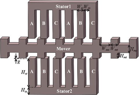
Figure 1 Structure of DSRLM.

Table 1 Key dimensions of DSRLM

Name	Parameter	Dimension (mm)
Stator tooth width	$W_{s t}$	21.5
Stator slot width	$W_{s s}$	18.5
Stator tooth length	$H_{s t}$	95.0
Stator yoke thickness	$H_{s y}$	23.5
Mover tooth width	$W_{m t}$	23.5
Mover slot width	$W_{m s}$	36.5
Mover tooth length	$H_{m t}$	17.5
Mover yoke thickness	$H_{m y}$	25.0
Air gap thickness	$g$	0.5
Laminated thickness	$L$	86.0

This paper investigates the velocity regulation control of a double-sided switched reluctance linear machine (DSRLM), shown in Fig. 1 and Table 1. A double closed-loop control algorithm is proposed, in which the acceleration loop is the inner loop, and the velocity loop is the outer loop. The PI regulator and the Fuzzy regulator are used in inner and outer loops alternately. Their regulation performances are compared with single-loop control algorithms.

2 CONTROLLER DESIGN

2.1 Design of Fuzzy regulator

The design process of a Fuzzy regulator can be divided into five steps.

(1) The first step is to determine the inputs and outputs of the regulator. In this paper, the two-dimensional Fuzzy regulator with double inputs and a single output (U) is selected to adjust the velocity or acceleration. Two inputs are the error (E) and the error variation (EC) of the variable.

(2) The second step is to determine the universe and the scale factor of every variable. In this paper, the basic universe of velocity is [ $-$ 1, 1] m/s, the basic universe of acceleration is [ $-$ 2, 2.5] m/s², and the basic universe of current reference values is [0, 6] A which always adds to a bias. The Fuzzy universe of the E, EC, and U is [ $-$ 6, 6].

(3) The third step is to determine the number of Fuzzy linguistic variables and their membership functions. In the design process of the Fuzzy regulator, what is the most important is to determine the number of Fuzzy linguistic variables and their membership functions. When the number of Fuzzy linguistic variables is large, the language rules would be more specific. Then its control effect will be more flexible and more accurate. However, sometimes the number is too large to implement and draw up its rules. Finally, under comprehensive consideration, there are 7 Fuzzy linguistic variables in total, which are sorted in terms of negative big (NB), negative medium (NM), negative small (NS), zero (ZE), positive small (PS), positive medium (PM), and positive big (PB). The frequently used membership functions are the triangular, trapezoidal, Gaussian, bell, and sigmoidal. The triangular membership function is selected in this paper owing to its concise notation and great interference immunity, which is shown in Fig. 2.

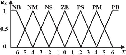
Figure 2 Triangular membership function.

Table 2 Language rules of the Fuzzy regulator

EC	E
	NB	NM	NS	ZE	PS	PM	PB
NB	NB	NB	NB	NB	NM	NS	ZE
NM	NB	NB	NB	NM	NS	ZE	PS
NS	NB	NB	NM	NS	ZE	PS	PM
ZE	NB	NM	NS	ZE	PS	PM	PB
PS	NB	NS	ZE	PS	PM	PB	PB
PM	NB	ZE	PS	PM	PB	PB	PB
PB	ZE	PS	PM	PB	PB	PB	PB

(4) The fourth step is to summarize the expert experience and express a series of language rules. The language rules of the Fuzzy regulator used in this paper are shown in Table 2. This step is the Fuzzy inference system (FIS). Some of the language rules of the Fuzzy regulator shown in Table 2 are introduced in this part briefly. For example, if E is NB, and EC is NB. It means that the value of the controlled object (velocity or acceleration) is much bigger than its reference value, and it has a trend to continue to expand this difference. Therefore, the output of the Fuzzy regulator should stop this trend and greatly reduce this difference. Related to the current acceleration reference values, they both should be reduced greatly. So, the output of the Fuzzy regulator is NB.

(5) The final step is defuzzification, which converts the Fuzzy values to the non-Fuzzy values according to a strategy. The centroid strategy is selected owing to its rationality. In the experiments, a two-dimensional decision table is established after the offline calculation according to the centroid strategy. Its curved surface is shown in Fig. 3. The fuzzification and defuzzification are expressed as

{\begin{matrix} E = i n t (e \cdot k e) \\ E C = i n t (e \cdot k e c) \\ u = U \cdot k u + c \end{matrix},

(1)

where e is the error between the controlled parameter and its reference value, ec is the error variation, u is the final output of the regulator, $k_{e}$ is the coefficient scale of e, $k_{e c}$ is the coefficient scale of ec, $k_{u}$ is the coefficient scale of u, c is a bias, and int() is a numerical function to get a numeric value down to the nearest integer.

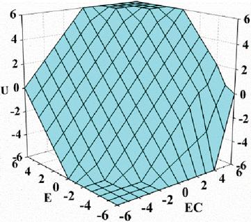
Figure 3 Offline calculation results of defuzzification.

2.2 Design of the PI regulator

The PI regulator is a widely used linear regulator. It implements the control of the object by the combination of the proportion and integral values of the deviation. The deviation is the difference between the given value and the actual value. The proportional link mainly affects the response speed and overshot value of the system. Generally, with the increase of the coefficient scale of the proportion link, the overshoot of the closed-loop system is increased, and the response speed of the system is accelerated. The integral link can help eliminate the steady state error of the system. The greater the coefficient scale of the integral link, the weaker the integral function, the smaller the overshoot of the closed-loop system and the lower the response speed of the system becomes. The equation of the principle of PI regulator can be expressed as

u = e \cdot k p + k i \cdot \int e d t,

(2)

where kp is the coefficient scale of the proportion link, ki is the coefficient scale of the integral link, and t is the time.

2.3 Single closed-loop control

The velocity single closed-loop control with PI regulator and Fuzzy regulator are investigated, respectively, whose control diagram is presented in Fig. 4. The velocity difference e is input in the PI/Fuzzy regulator which outputs the corresponding current reference value $I_{r e f}$ . The phase currents $i_{a1}, i_{a2}, i_{b1}, i_{b2}, i_{c1}$ , and $i_{c2}$ are compared with the reference current of every phase, respectively in the hysteresis comparator. An AND logic operation is conducted between its output and the output of the position judgment to control the switches on the power converter. The mover of the DSRLM runs and feeds back the real-time velocity v to the regulator, and position x to the position judgment link with the position sensor.

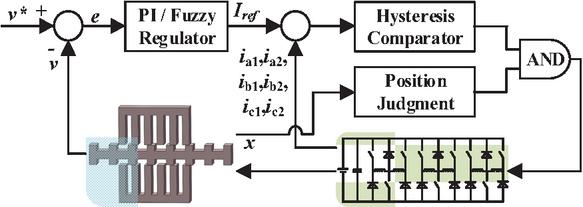
Figure 4 Diagram of velocity single closed-loop control.

2.4 Double closed-loop control

In the velocity-acceleration double closed-loop control, the PI regulator and the Fuzzy regulator are used in inner and outer loops alternately, whose diagram is presented in Fig. 5.

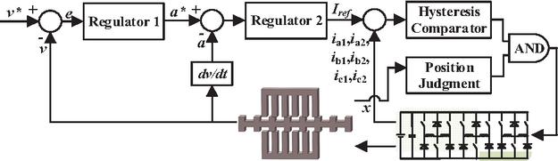
Figure 5 Diagram of velocity-acceleration double closed-loop control.

The velocity loop is the outer loop which outputs the acceleration reference values according to the velocity difference. The acceleration loop is the inner loop that outputs the current reference values according to the acceleration difference. The following process is the same as the velocity single closed-loop diagram. An AND logic operation is conducted between the hysteresis comparator’s output and the output of the position judgment to control the switches on the power converter. The deviation between real-time velocity and the given velocity is input to regulator 1, and position x to the position judgment link with the position sensor. The acceleration of the mover is achieved after the differential calculation of velocity, and it is fed back to regulator 2 in the inner loop.

3 SIMULATION RESULTS AND ANALYSIS

As shown in Fig. 5, the PI regulator and the Fuzzy regulator are used as regulator 1 and regulator 2 alternately. There are four double closed-loop controllers in total. The simulation results of four double closed-loop controllers and two single-loop controllers are conducted. Under no load and 24 V power supply, the model of the DSRLM is established by the Fourier modeling method proposed in [21]. Two simulation results of 0.4 m/s are shown in Fig. 6.

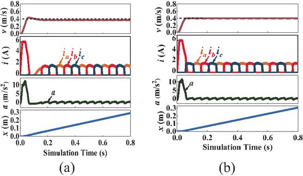
Figure 6 Simulation results under 0.4 m/s given velocity: (a) PI controller and (b) Fuzzy controller.

The simulation results of 0.6 m/s are shown in Fig. 7. In these figures, v is the mover velocity. Owing to the symmetry of double-sided currents, the currents of only one side are given, where $i_{a}$ , $i_{b}$ , and $i_{c}$ are the current values of phases A1, B1, and C1, respectively, arf is the acceleration reference output by the regulator 1, a is the simulated mover acceleration, and x is the mover position.

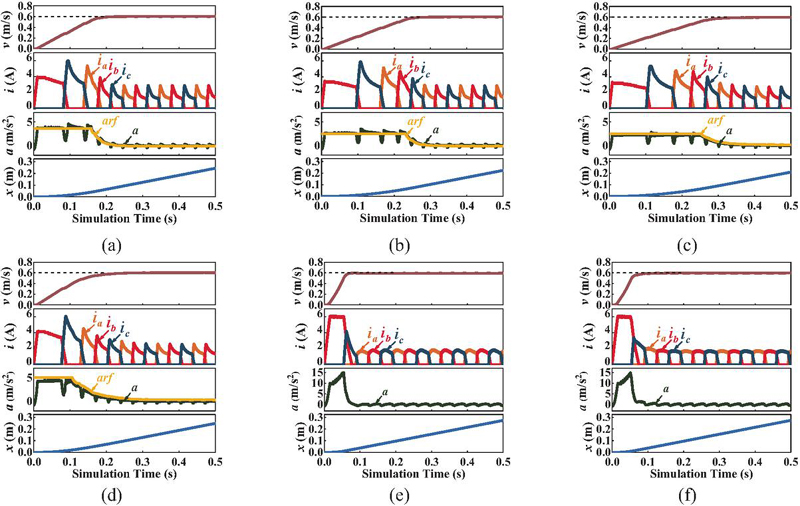
Figure 7 Simulation results under given velocity 0.6 m/s: (a) Fuzzy-Fuzzy controller, (b) PI-Fuzzy controller, (c) PI-PI controller, (d) Fuzzy-PI controller, (e) PI controller, (f) Fuzzy controller.

In the simulation results of Fuzzy-Fuzzy double closed-loop velocity regulation, there is no overshoot in the process of velocity regulation, and the arising time and steady-state error of the controller are about 0.232 s and 0.013 m/s. In the simulation results of PI-Fuzzy double closed-loop velocity regulation, there is no overshoot, and its arising time and steady-state error of the controller are about 0.300 s and 0.024 m/s. Also, there is no overshoot in the process of velocity regulation with the PI-PI controller. Its arising time and steady-state error of the controller are about 0.411 s and $-$ 0.006 m/s. The simulation results of Fuzzy-PI double closed-loop velocity regulation show that there is no overshoot in the process of velocity regulation with the Fuzzy-PI controller, and its arising time and steady-state error of the controller are about 0.268 s and 0.05 m/s. The simulation results of PI single closed-loop velocity regulation and Fuzzy single closed-loop velocity regulation are shown in Figs. 7 (e) and 7 (f), respectively. With the PI regulator, when the given velocity is 0.4 m/s, the arising time and static state error of the controller are about 0.063 s and 0.035 m/s, and there is an overshoot which is about 0.035 m/s. When the given velocity is 0.6 m/s, the arising time and steady-state error of the controller are about 0.080 s and $-$ 0.009 m/s, and there is no overshoot. With a Fuzzy regulator, it can be seen that there is no overshoot in the velocity regulation results. When the given velocity is 0.4 m/s, the arising time and static state error of the controller are about 0.056 s and $-$ 0.006 m/s. When the given velocity is 0.6 m/s, the arising time and static state error of the controller are about 0.115 s and $-$ 0.005 m/s.

The control performances of the six controllers are compared in Table 3. The overshoot, arising time, and steady-state error are quantized at two different given velocities. It can be seen that two single closed-loop controllers have a shorter arising time than four double closed-loop controllers, but the PI controller shows an overshoot when the given velocity is 0.4 m/s. In many applications, a small overshoot may cause huge damage to the whole system. Therefore, although four double closed-loop controllers have relatively longer arising time than PI controllers, they are still thought better for no overshoot. Among the four double closed-loop controllers, it is apparent that the arising times of the PI-Fuzzy controller and PI-PI controller are larger than those of the Fuzzy-Fuzzy controller and Fuzzy-PI controller. The Fuzzy-PI controller is better than the Fuzzy-Fuzzy controller in steady state error but is worse in arising time. Thus, further comparisons of the Fuzzy controller, Fuzzy-Fuzzy controller, and Fuzzy-PI controller should be conducted by variable-given velocity tests. These conclusions obtained by simulations should be verified by experiments.

Table 3 Velocity regulation performance comparisons of the six controllers in simulations

Controller	Given	Arising	Steady-	Overshoot
	Velocity	Time	State	(%)
	(m/s)	(s)	(m/s)
Fuzzy-	0.4	0.159	0.005	0
Fuzzy	0.6	0.232	0.005	0
PI-Fuzzy	0.4	0.188	0.002	0
	0.6	0.300	0.002	0
PI-PI	0.4	0.318	-0.006	0
	0.6	0.411	-0.006	0
Fuzzy-PI	0.4	0.219	0.002	0
	0.6	0.268	0.001	0
PI	0.4	0.063	0.035	8.875
	0.6	0.080	-0.009	0
Fuzzy	0.4	0.060	-0.006	0
	0.6	0.115	-0.005	0

4 EXPERIMENTAL VERIFICATIONS

4.1 Hardware platform and coefficients of controllers

The whole velocity regulation system is shown in Fig. 8, which includes a DSRLM prototype, an RT-LAB digital controller, an isolator, a drive circuit, a sampling circuit, a linear encoder, and a power converter. In experiments with different controllers, coefficients are different. There are two main control objects in this paper, which are the mover velocity and its acceleration. The basic universe of velocity is [ $-$ 1, 1] m/s, the basic universe of acceleration is [ $-$ 2, 2.5] m/s², and the basic universe of current reference values is [0, 6] A which always adds to a bias, thus some coefficients in the Fuzzy regulator and PI regulator can be determined. For example, when the Fuzzy regulator is used in the outer loop, its output u is the acceleration reference value. And the Fuzzy universe of the E, EC, and U is [ $-$ 6, 6], so the value of $k_{u}$ in Fig. 9 (a) is 2.25/6, and the bias is 0.25. The purpose is to change the universe of the output of the Fuzzy to the universe of the acceleration. Similarly, when the Fuzzy regulator is used in the inner loop, its output u is the current reference value, so the value of $k_{u}$ in Fig. 9 (a) is 3/6, and the bias is 3. When the PI regulator is used in the outer loop, its output $u$ is the acceleration reference value, so it sets $-$ 2 as the lower limit and 2.5 as the upper limit in the saturation in Fig. 9 (b). When the PI regulator is used in the inner loop, its output u is the current reference value, so it sets 0 as the lower limit and 6 as the upper limit in the saturation in Fig. 9 (b). Then detailed coefficients in different controllers used in experiments are summarized in Table 4. Besides, the flux-linkage of the DSRLM is calculated by the Fourier series modeling method, which is the same as section 3.

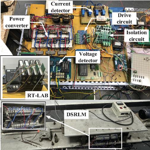
Figure 8 Prototype and hardware platform.

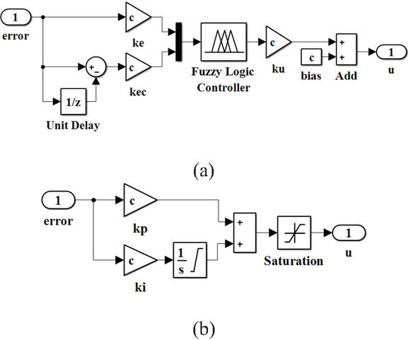
Figure 9 Regulator modules in Simulink: (a) Fuzzy regulator and (b) PI regulator.

Table 4 Detailed coefficients in different controllers

Controller	PI-PI Controller	PI-Fuzzy Controller	Fuzzy-PI Controller	Fuzzy-Fuzzy Controller
Regulator 1 in	$k_{p} = 16$	$k_{p} = 16$	$k_{e} = 20$	$k_{e} = 20$
the outer loop	$k_{i} = 0.05$	$k_{i} = 0.05$	$k_{e c} = 2.6$	$k_{e c} = 2.6$
	Lower limit $=$ $-$ 2	Lower limit $=$ $-$ 2	$k_{u} = 2.25 / 6$	$k_{u} = 2.25 / 6$
	Upper limit $=$ 2.5	Upper limit $=$ 2.5	bias $=$ 0.25	bias $=$ 0.25
Regulator 2 in	$k_{p} = 6.5$	$k_{e} = 35$	$k_{p} = 6.5$	$k_{e} = 35$
the inner loop	$k_{i} = 0.03$	$k_{e c} = 2.8$	$k_{i} = 0.03$	$k_{e c} = 2.8$
	Lower limit $=$ 0	$k_{u} = 3 / 6$	Lower limit $=$ 0	$k_{u} = 3 / 6$
	Upper limit $=$ 6	bias $=$ 3	Upper limit $=$ 6	bias $=$ 3

4.2 Experiments

The velocity regulation experiments with different controllers are conducted using the shown hardware platform. In these results, $a_{r f}$ is the acceleration reference value output by regulator 1. The results of the Fuzzy-Fuzzy double closed-loop controller are presented in Fig. 10 (a). It can be observed that there is no overshoot in the velocity regulation process with this controller. When the given velocity is 0.6 m/s, the arising time and steady-state error of the controller are approximately 0.160 s and 0.038 m/s. The results of velocity regulation experiments with the PI-Fuzzy double closed-loop controller are shown in Fig. 10 (b). There is no overshoot in the velocity regulation process. When the given velocity is 0.6 m/s, the arising time and steady-state error of the controller are about 0.266 s and $-$ 0.010 m/s. Figure 10 (c) presents the results of velocity regulation experiments with the PI-PI double closed-loop controller at a given velocity of 0.6 m/s. There is no overshoot in the velocity regulation process in the figure, and the arising time and steady-state error of the controller are approximately 0.262 s and 0.021 m/s. The results of velocity regulation experiments with the Fuzzy-PI double closed-loop controller are shown in Fig. 10 (d). It can be seen that there is no overshoot in the velocity regulation process when the given velocity is 0.6 m/s. Its arising time and steady-state error of the controller are about 0.250 s and 0.009 m/s. Velocity regulation experiments with the PI single closed-loop controller are also conducted. Their results are shown in Figs. 11 (a) and 11 (b). When the given velocity is 0.4 m/s, the arising time and steady-state error of the controller are about 0.060 s and $-$ 0.049 m/s, with approximately 14.325% overshoot. When the given velocity is 0.6 m/s, the arising time and steady-state error of the controller are about 0.096 s and $-$ 0.016 m/s, and there is no overshoot. The velocity regulation experiments with the Fuzzy single closed-loop controller are shown in Fig. 12. There is no overshoot in the velocity regulation process when the given velocity is 0.6 m/s. Its arising time and steady-state error of the controller are about 0.150 s and 0.010 m/s.

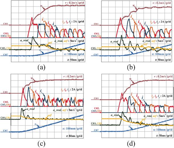
Figure 10 Experiment results of different controllers under 0.6 m/s: (a) Fuzzy-Fuzzy controller, (b) PI-Fuzzy controller, (c) PI-PI controller, (d) Fuzzy-PI controller.

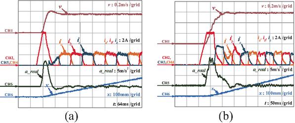
Figure 11 Experiment results of PI controller: (a) under 0.4 m/s and (b) under 0.6 m/s.

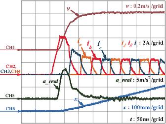
Figure 12 Experiment results of Fuzzy controller under 0.6 m/s.

On the other hand, from the invariable given velocity tests, it can be found that the single closed-loop Fuzzy controller, the double closed-loop Fuzzy-Fuzzy controller, and the double closed-loop Fuzzy-PI controller have better performances among the six controllers. To further investigate their stability and anti-disturbance ability, the given velocity is changed from 0.4 m/s to 0.6 m/s suddenly, and the velocity regulation processes of the three controllers are shown in Fig. 13.

Figure 13 (a) is the given velocity step test results of the Fuzzy controller. It is shown that the real-time velocity follows the given velocity well, and it responds quickly. The parameters in a single closed-loop controller are less than those in a double closed-loop controller, so the parameter adjustment of the Fuzzy controller is easy. Figure 13 (b) is the variable given the velocity test results of the Fuzzy-Fuzzy controller, which shows that it responds slowly, and the velocity waveform is not stable. It indicates that the Fuzzy-Fuzzy cannot work well in variable-given velocity tests. Figure 13 (c) is the variable given the velocity test results of the Fuzzy-PI controller. It can be seen that the real-time velocity follows the given velocity well with a quick response.

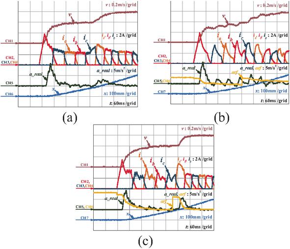
Figure 13 Variable given velocity test results: (a) Fuzzy controller, (b) Fuzzy-Fuzzy controller, (c) Fuzzy-PI controller.

Table 5 Velocity regulation performance comparisons of the six controllers in experiments

Controller	Given	Arising	Steady-State	Overshoot (%)	$α$ (%)
	Velocity (m/s)	Time (s)	Error (m/s)		Invariable	Variable
Fuzzy-	0.4	0.151	0.012	0	7.77	9.9
Fuzzy	0.6	0.160	0.038	0	7.52
PI-Fuzzy	0.4	0.213	0.028	0	7.48	–
	0.6	0.266	$-$ 0.010	0	8.11
PI-PI	0.4	0.260	0.022	0	3.79	–
	0.6	0.262	0.021	0	3.86
Fuzzy-PI	0.4	0.192	0.001	0	3.99	4.03
	0.6	0.250	0.009	0	3.94
PI	0.4	0.060	$-$ 0.049	14.325	4.56	–
	0.6	0.096	$-$ 0.016	0	4.11
Fuzzy	0.4	0.096	0.005	0	3.95	4.08
	0.6	0.150	0.010	0	3.93

4.3 Analysis

The control performances of the six controllers shown in the experiments are compared in Table 4. In the arising time column, the values of the PI controller at 0.4 m/s and 0.6 m/s are 0.060 s and 0.096 s, and those of the Fuzzy controller at 0.4 m/s and 0.6 m/s are 0.096 s and 0.150 s. They are shorter than those of four double closed-loop controllers under the same given velocity. That means that single closed-loop controllers are more flexible, and they have quicker response speeds. However, in the PI controller, experiment results appear unexpected steady-state errors and a 14.325% overshoot at a given velocity of 0.4 m/s. Among four double closed-loop controllers, the Fuzzy-Fuzzy controller has the shortest arising times. In the steady state error column, the values of the Fuzzy-PI controller can be maintained within 0.01 m/s. It is better than other controllers, including single closed-loop controllers and double closed-loop controllers. The static state errors in these experiments may be caused by the impacts of the coefficients of these controllers. DSRLM system is a nonlinear system. Its motion stroke is only 380 mm, which is a limited distance so the real-time regulation of these coefficients is difficult to realize. In general, the coefficients of these controllers are chosen to apply to a majority of situations in the SRLM velocity regulation system. Under these situations, these controllers can perform well without changing these coefficients. Nevertheless, achieving the optimal outcomes consistently is challenging, and static state errors might emerge in certain circumstances due to the coefficients. However, it can be observed from Tables 3 and 5 that significant static state errors rarely occur, indicating that the majority of the results are acceptable.

Comparing Tables 3 and 5, both the simulated results and the tested results of the PI controller appear big steady-state errors at a given velocity of 0.4 m/s. All steady-state errors of tested results are greater than those of simulated results. In addition, the arising times of tested results are different from those of simulated results. These differences between tested results and simulated results may be caused by the calculated frequency of the real-time simulator, the accuracy of flux linkage curves used in Fourier series nonlinear modeling, or the effect of mutual coupling characteristics between phase to phase.

The smaller the smoothness coefficient $α$ , the better the stability of the system. In Table 5, “Invariable” shows the smoothness coefficients $α$ of invariable given velocity tests, and “Variable” shows the smoothness coefficients $α$ of the variable given velocity tests. The $α$ values of the Fuzzy-Fuzzy controller and PI-Fuzzy controller are bigger than those of the other four controllers in invariable given velocity tests. The $α$ values of the Fuzzy-PI controller keep the same level as the Fuzzy controller. The smoothness of real-time velocity with Fuzzy-PI controller and Fuzzy controller is great, both in invariable given velocity tests or variable given tests. The smoothness of real-time velocity with a Fuzzy-PI controller is better than that with a Fuzzy controller in variable-given velocity tests. In its process of parameter adjustment, we found that the Fuzzy-PI controller is flexible and easy to adjust. Above all, in the further velocity regulation of DSRLM, the Fuzzy-PI controller can be chosen.

5 CONCLUSION

In a velocity regulation system of a DSRLM, the velocity single closed-loop control employing either the PI regulator or the Fuzzy regulator is contrasted with the velocity-acceleration double closed-loop control in this paper. The velocity regulation control is executed using an RT-LAB digital controller. The velocity regulation experiments are carried out, and corresponding simulations are established in MATLAB. Moreover, the modules in MATLAB/Simulink are presented. Another contribution of this paper lies in comparing and analyzing the performances of different velocity regulation controllers on SRLMs through simulations and experiments. The establishment processes of different controllers are introduced in detail, and their specifications are provided. Through a succession of velocity regulation tests, the conclusion can be drawn that the Fuzzy-PI controller possesses the optimal velocity regulation performance in the DSRLM. These simulated and experimental experiences can serve as a reference for velocity regulation research on other SRLMs. Although the proposed velocity–acceleration double closed-loop control strategy demonstrates satisfactory performance for DSRLM velocity regulation, several aspects warrant further investigation. First, the current controller design relies on empirically tuned PI and Fuzzy parameters, and future work will focus on developing adaptive or self-tuning mechanisms to enhance robustness under varying operating conditions. Second, the strong nonlinearities and axial end effects inherent to SRLMs are not explicitly compensated in the control law; incorporating end-effect-aware models or data-driven compensation strategies is a promising direction. In addition, performance evaluation in this study is limited to low-speed and constant-load conditions. Future experimental validation under wider speed ranges, load disturbances, and parameter uncertainties will be conducted. Finally, comparisons with more advanced control approaches, such as model predictive control or learning-based methods, will be explored to further improve dynamic performance and broaden the applicability of the proposed framework.

ACKNOWLEDGMENTS

This work is supported by the Shenzhen Collaborative Innovation Special Plan International Cooperation Research Project under Grant GJHZ2024021811 4300002.

REFERENCES

[1] J. B. Bartolo, M. Degano, J. Espina, and C. Gerada, “Design and initial testing of a high-speed 45-kW switched reluctance drive for aerospace application,” IEEE Transactions on Industrial Electronics, vol. 64, no. 2, pp. 988–997, Feb. 2017.

[2] X. Cao, H. Yang, L. Zhang, and Z. Q. Deng, “Compensation strategy of levitation forces for single-winding bearingless switched reluctance motor with one winding total short circuited,” IEEE Transactions on Industrial Electronics, vol. 63, no. 9, pp. 5534–5546, Sep. 2016.

[3] H. Chen, H. Yang, Y. X. Chen, and H. H. C. Iu, “Reliability assessment of the switched reluctance motor drive under single switch chopping strategy,” IEEE Transactions on Power Electronics, vol. 31, no. 3, pp. 2395–2408, Mar. 2016.

[4] A. Chiba, K. Kiyota, N. Hoshi, M. Takemoto, and S. Ogasawara, “Development of a rare-earth-free SR motor with high torque density for hybrid vehicles,” IEEE Transactions on Energy Conversion, vol. 30, no. 1, pp. 175–182, Mar. 2015.

[5] H. Chen, Q. L. Wang, and H. H. C. Iu, “Acceleration closed-loop control on a switched reluctance linear launcher,” IEEE Transactions on Plasma Science, vol. 41, no. 5, pp. 1131–1137, May 2013.

[6] D. H. Wang, X. F. Du, D. X. Zhang, and X. H. Wang, “Design, optimization, and prototyping of segmental-type linear switched-reluctance motor with a toroidally wound mover for vertical propulsion application,” IEEE Transactions on Industrial Electronics, vol. 65, no. 2, pp. 1865–1874, Feb. 2018.

[7] J. F. Pan, N. C. Cheung, and Y. Zou, “Design and analysis of a novel transverse-flux tubular linear machine with gear-shaped teeth structure,” IEEE Transactions on Magnetics, vol. 48, no. 11, pp. 3339–3343, Nov. 2012.

[8] Z. Zhang, N. C. Cheung, K. W. E. Cheng, X. D. Xue, and J. K. Lin, “Direct instantaneous force control with improved efficiency for four-quadrant operation of linear switched reluctance actuator in active suspension system,” IEEE Transactions on Vehicular Technology, vol. 61, no. 4, pp. 1567–1576, May 2012.

[9] J. F. Pan, Y. Zou, G. Z. Cao, N. C. Cheung, and B. Zhang, “High-precision dual-loop position control of an asymmetric bilateral linear hybrid switched reluctance motor,” IEEE Transactions on Magnetics, vol. 51, no. 11, Nov. 2015.

[10] J. H. Du, D. L. Liang, L. Y. Xu, and Q. F. Li, “Modeling of a linear switched reluctance machine and drive for wave energy conversion using matrix and tensor approach,” IEEE Transactions on Magnetics, vol. 46, no. 6, pp. 1334–1337, Jun. 2010.

[11] D. H. Wang, C. L. Shao, X. H. Wang, and C. H. Zhang, “Performance characteristics and preliminary analysis of low cost tubular linear switch reluctance generator for direct drive WEC,” IEEE Transactions on Applied Superconductivity, vol. 26, no. 7, Oct. 2016.

[12] N. Alibeji and N. Sharma, “A PID-type robust input delay compensation method for uncertain Euler-Lagrange systems,” IEEE Transactions on Control Systems Technology, vol. 25, no. 6, pp. 2235–2242, Nov. 2017.

[13] Y. D. Song, X. C. Huang, and C. Y. Wen, “Robust adaptive fault-tolerant PID control of MIMO nonlinear systems with unknown control direction,” IEEE Transactions on Industrial Electronics, vol. 64, no. 6, pp. 4876–4884, Jun. 2017.

[14] T. Mahto and V. Mukherjee, “Fractional order fuzzy PID controller for wind energy-based hybrid power system using quasi-oppositional harmony search algorithm,” IET Generation Transmission & Distribution, vol. 11, no. 13, pp. 3299–3309, Sep. 2017.

[15] X. Chen, J. Hu, M. Wu, and W. H. Cao, “T-S fuzzy logic based modeling and robust control for burning-through point in sintering process,” IEEE Transactions on Industrial Electronics, vol. 64, no. 12, pp. 9378–9388, Dec. 2017.

[16] D. Sun, Q. F. Liao, and H. L. Ren, “Type-2 fuzzy modeling and control for bilateral teleoperation system with dynamic uncertainties and time-varying delays,” IEEE Transactions on Industrial Electronics, vol. 65, no. 1, pp. 447–459, Jan. 2018.

[17] S. Demirbas, “Self-tuning fuzzy-PI-based current control algorithm for doubly fed induction generator,” IET Renewable Power Generation, vol. 11, no. 13, pp. 1714–1722, Nov. 2017.

[18] M. A. Fnaiech, “A measurement-based approach for speed control of induction machines,” IEEE Journal of Emerging and Selected Topics in Power Electronics, vol. 2, no. 2, pp. 308–318, Jun. 2014.

[19] M. H. Khooban, M. Sadeghi, T. Niknam, and F. Blaabjerg, “Analysis, control and design of speed control of electric vehicles delayed model: Multi-objective fuzzy fractional-order controller,” IET Science Measurement & Technology, vol. 11, no. 3, pp. 249–261, May 2017.

[20] A. Ashouri-Zadeh, M. Toulabi, S. Bahrami, and A. M. Ranjbar, “Modification of DFIG’s active power control loop for speed control enhancement and inertial frequency response,” IEEE Transactions on Sustainable Energy, vol. 8, no. 4, pp. 1772–1782, Oct. 2017.

[21] I. Mahmoud and H. Rehaoulia, “Nonlinear modelling improvement approach for linear actuator,” in Proc. International Conference on Control, Automation and Diagnosis (ICCAD), Hammamet, Tunisia, pp. 482–486, Jan. 2017.

BIOGRAPHIES

Hao Chen (Senior Member, IEEE) received his B.S. and Ph.D. degrees in electrical engineering from the Department of Automatic Control, Nanjing University of Aeronautics and Astronautics, Nanjing, China, in 1991 and 1996, respectively. In 1998, he became an Associate Professor at the School of Information and Electrical Engineering, China University of Mining and Technology, Xuzhou, where he has been a Professor since 2001. From 2002–2003, he was a Visiting Professor at Kyungsung University, Busan, Korea. Since 2008, he has also been an Adjunct Professor at the University of Western Australia, Perth, Australia. He is the author of one book and has authored more than 300 papers. He is a holder of 15 US patents, 23 Australian patents, one Danish patent, seven Canadian patents, three South African patents, 10 Russian patents, 86 Chinese invention patents, and six Chinese Utility Model patents.

Sergei Brovanov received the engineer degree from the Industrial Electronics Department, Novosibirsk Electrotechnical Institute in 1987. In 1999, he became an Associate Professor in the Industrial Electronics Department, Novosibirsk State Technical University, where he has been a Professor since 2013. In 2004, he was a Visiting Professor at Ulsan University, South Korea. He is the author of one book and has authored more than 150 papers. He has 17 Russian patents. His current research interests include semiconductor converters, vector PWM of multilevel NPC converters, and semiconductor converters for electrical energy storage systems. In 1996–1997, he was awarded a scholarship from the Swiss Academy of Engineering Sciences. In 2023, he was awarded the State Prize of the Novosibirsk Region for the development of intelligent power electronic systems and devices. Brovanov currently is a professor in the electronics and electrical engineering Department at Novosibirsk State Technical University.

Javokhir Toshov received the B.S. degree from Navoi State Mining Institute, Navoi, Uzbekistan, in 1999, M.S. degree from Tashkent State Technical University, Tashkent, in 2002, Dr.Sci. in 2017, and Professor of the Tashkent State Technical University since 2020. He has about 250 published and reviewed works. His current research interests include drilling control for drilling operations, as well as electrical installations and motors for mining equipment. For many years he worked as the dean of the energy faculty, and today he works as the head of the department at Tashkent State Technical University.

Jinfu Liu received the B.S. degree in Mechanical and Electrical Engineering, from Northeast Forestry University, Harbin, Heilongjiang, China, in 2017, M.S. degree from the School of Electrical Engineering, China University of Mining and Technology, Xuzhou, Jiangsu, in 2021, and is currently pursuing a Ph.D. degree in electrical engineering at the China University of Mining and Technology, Xuzhou. His research interests include switched reluctance linear motor control, ocean wave power generation, and electric vehicles.

Xing Wang received the B.S. degree from China University of Mining and Technology, Xuzhou Jiangsu, China, in 1996, and M.S. degree from China University of Mining and Technology, Xuzhou Jiangsu, in 1999. In 2007, she became an Associate Professor with China University of Mining and Technology, Xuzhou, China. She is a holder of four US Patents, nine Australian Patents, two Canadian Patents, four Russian Patents, 12 Chinese Invention Patents, three Chinese Utility Model Patents, and has authored 15 papers.

Antonino Musolino received his Ph.D. degree in electrical engineering from the University of Pisa, Pisa, Italy, in 1994. He is currently a Full Professor of electrical machines at the University of Pisa. He has co-authored more than 130 papers published in international journals/conferences. He holds three international patents in the field of magnetorheological devices. His current research activities are focused on linear electromagnetic devices, motor drives for electric traction, and the development of analytical and numerical methods in electromagnetics. Musolino was involved in the organization of several international conferences, where he has served as the session chairman and an organizer, and as a member of the editorial board.

Nurkhat Zhakiyev is a computer modeler of energy systems and physical processes. Developed modeling tools and data science for Energy and Environment economics. Climate Change Mitigation Analyst. He is now a Senior Research, Assoc. Prof., Head of the Department of Science and Innovation, Astana IT University.

Murat Shamiyev received the B.S. and M.S. degrees from Tashkent State Technical University, Tashkent, Uzbekistan, in 1999 and 2001, respectively. He served as a Professor’s Assistant at the Department of Electromechanics and Electrotechnology, Faculty of Energy, Tashkent State Technical University from 2001 to 2005. Following that, he held the position of Head Specialist at Azia Triol Joint Venture (Russia and Uzbekistan) from 2005 to 2007. Subsequently, he served as a Technical Director at “Энерготежаш” LLC from 2007 to 2010. He then took on the role of Director at Techno Energo Group LLC. Currently, he holds the position of Head Engineer at Techno Energo Group LLC.

Abror Abidovich Pulatov is the head of the Department of Electrical Machinery and Electrical Technology of Tashkent State Technical University. His main monographs include “Thermal Operating Conditions of Induction Crucible Furnaces,” “Instruction Manual for Electrical Equipment and Power Supply in Mining Enterprises,” “Guide to Laboratory Work in Electrical Technology Fundamentals,” and “Design and Operation of Electrical Technology Devices.” His main research directions include the research on inductors of smelting devices, and monitoring, control and regulation of asynchronous motor devices. He is a Member of the Academic Committee of the International Joint Research Center for New Energy Electric Vehicle Technology and Equipment in Central and Eastern European Countries of the Ministry of Science and Technology of China, member of the Academic Committee of the International Cooperation Joint Laboratory for New Energy Generation and Electric Vehicles of Jiangsu Province’s Universities, and member of the New Energy Generation and Electric Vehicles Foreign Expert Studio in Jiangsu Province.

EC	E
	NB	NM	NS	ZE	PS	PM	PB
NB	NB	NB	NB	NB	NM	NS	ZE
NM	NB	NB	NB	NM	NS	ZE	PS
NS	NB	NB	NM	NS	ZE	PS	PM
ZE	NB	NM	NS	ZE	PS	PM	PB
PS	NB	NS	ZE	PS	PM	PB	PB
PM	NB	ZE	PS	PM	PB	PB	PB
PB	ZE	PS	PM	PB	PB	PB	PB

EC	E
	NB	NM	NS	ZE	PS	PM	PB
NB	NB	NB	NB	NB	NM	NS	ZE
NM	NB	NB	NB	NM	NS	ZE	PS
NS	NB	NB	NM	NS	ZE	PS	PM
ZE	NB	NM	NS	ZE	PS	PM	PB
PS	NB	NS	ZE	PS	PM	PB	PB
PM	NB	ZE	PS	PM	PB	PB	PB
PB	ZE	PS	PM	PB	PB	PB	PB

EC	E
	NB	NM	NS	ZE	PS	PM	PB
NB	NB	NB	NB	NB	NM	NS	ZE
NM	NB	NB	NB	NM	NS	ZE	PS
NS	NB	NB	NM	NS	ZE	PS	PM
ZE	NB	NM	NS	ZE	PS	PM	PB
PS	NB	NS	ZE	PS	PM	PB	PB
PM	NB	ZE	PS	PM	PB	PB	PB
PB	ZE	PS	PM	PB	PB	PB	PB