Inversion Method of Lightning Current Distribution on a Surface Conductor Represented by Thin Lines

Zemin Duan $^{1}$ , Chen Tong $^{1}$ , Yeyuan Huang $^{2,3,4}$ , Xinping Li $^{5}$ , Shanliang Qiu $^{2,3,4}$ ,Xiaoliang Si $^{2,3,4}$ , Yan Wei $^{1}$ , and Yao Ling $^{1}$

¹School of Electrical Engineering and Automation
Hefei University of Technology, Hefei 230009, China
duanzemin@yeah.net, 2018110388@mail.hfut.edu.cn, 2020170474@mail.hfut.edu.cn, 862060425@qq.com

²National Key Laboratory of Electromagnetic Information Control and Effects
Hefei 230031, China
yeyuan_huang@outlook.com, wobenshanliang1983@163.com, sixiaoliang1985@126.com

³Key Laboratory of Strong Electromagnetic Environment Protection Technology
Hefei 230031, China

⁴Key Laboratory of Aircraft Lightning Protection of Anhui Province
Hefei 230031, China

⁵School of Mathematics
Hunan Institute of Science and Technology, Yueyang 414006, China
xpli@hnist.edu.cn

Submitted On: December 4, 2024; Accepted On: March 6, 2025

ABSTRACT

Electromagnetic simulation and pre-analysis of electromagnetic compatibility for lightning effects are important. It is difficult to estimate the surface current of surface structures represented by thin lines. In this study, we simplified the partial element equivalent circuit (PEEC) equation and deduced an equation for the magnetic field based on the thin-line representation method. An inversion method was used to determine the surface current in a frequency-domain PEEC. Parallel computing technology was used to improve the inversion efficiency. Additionally, the capacitive and inductive characteristics of the elements of Darney’s circuit method were developed for PEEC. The results were compared with calculations using the finite integration technique. The application of the thin-line representation method was broadened, and its efficiency has been improved.

Index Terms: Lightning current distribution, magnetic field distribution, partial element equivalent circuit, thin-line representation method.

I. INTRODUCTION

As the complexity and intensity of the electromagnetic environment increase, electromagnetic simulation and pre-analysis [1–5] become more important, especially in the analysis of structural surface current distributions and magnetic field distributions [6, 7–13]. The distribution of the lightning surface current andmagnetic field is important, particularly for lightning protection.

Among electromagnetic simulation methods, the thin-line representation method [14–16], proposed in 1986, is well known for its high efficiency. In recent years, it has attracted the attention of scholars because it can rapidly perform sensitivity analyses [17–20]. The thin-line representation has been applied for solving electromagnetic problems under the framework of the classical circuit [21, 22] and partial element equivalent circuit (PEEC) [23]. The framework of the classical circuit described in the previous study, also called Darney’s circuit method, has been extended for electromagnetic compatibility and electromagnetic interference (EMC/EMI) [24]. The PEEC framework described above is called the one-dimensional (1D)-PEEC.

Thin-line representation is likely to become an important preparatory step for future electromagnetic simulations[25]. It is mainly used to solve difficulties related to structures composed of lines such as high-voltage transmission towers and grounding grids[26–28]. Li analyzed the shielding effect of modern buildings with wire mesh structures in a lightning environment [29]. Ye et al. proposed an efficient full-wave PEEC equation for thin-line structures in a lossy ground for transient lightning analysis [27]. Prost et al.conducted thin-line modeling of A320 landing gear [30]. However, these studies only considered the application of the thin-line representation when the structure was a thin wire rather than surface structures.

For surface structures, the structure is represented by parallel lines, or only the cross-section is analyzed [25]. Several studies have considered the application of the thin-line representation for surface structures. Lv used thin-line representation to analyze the scattering of an aircraft [31]. Torchio used a method based on PEEC to analyze fast voltage transient and toroidal coils in a JT-60SA fusion reactor [23, 32]. This study showed that the thin-line representation could simulate full-wave electromagnetic processes using appropriate solution methods. However, there are few studies on current distribution in lightning environments.

Regarding the lightning current distribution of surface structures, Parmantier et al. analyzed the cable response in a lightning environment under a simplified two-dimensional (2D) cross-section [25]. In these studies, the current was restricted to the flow perpendicular to the cross-section [21, 22]. Although they simulated the proximity effect of the lightning current, the study of the lightning current distribution involves far more than that.

The difficulty in inverting the surface current distribution of a surface structure lies in determining the height of the magnetic field strength, which is associated with the surface current. In the finite-difference time-domain (FDTD), the surface current can be calculated using the magnetic field near the conductor [33]. Unlike the FDTD, free space is not meshed regardless of Darney’s circuit method or 1D-PEEC. Therefore, the surface current cannot be calculated directly using a magnetic field.

In this study, PEEC equations were simplified by analyzing the difference in the PEEC in a situation where the surface structure is represented by thin lines. The influences of simplification and delay on the results were also analyzed. An inversion method for the surface current distribution was proposed by calculating the average value of the magnetic field strength of all surface elements. In addition, parallel computing was used to improve the efficiency of the method. Finally, the capacitance-inductance duality characteristics in classical circuit theory were extended to PEEC.

II. PEEC METHOD

The PEEC method is an integration method that introduces the concept of partial elements and performs circuit interpretation on the electric field integral equation (EFIE) through the resistance, partial inductance, and potential coefficient [23]. Thus, the resulting equivalent circuit is studied by the Tableau analysis method or by means of Spice-like circuit solvers in both time and frequency domains [23]. It is a full-wave method based on EFIE and is widely used in EMC/EMI and other research fields.

The application of the 1D-PEEC to aircraft lightning effects differs from that of thin-wire structures such as high-voltage towers, grounding grids, and down conductors. This difference is analyzed below. If the conductors are thin-wire structures, the thin-wire representation is very simple, as shown in Figs. 1 (a) and (b). When the computational domain contains soil, the half-space of the soil [27] and air must be considered.

For surface structures such as landing gear and aircraft fuselages, the structure is simplified, or only the cross-section is discretized, as shown in Figs. 1 (e)and (f) [25, 30].

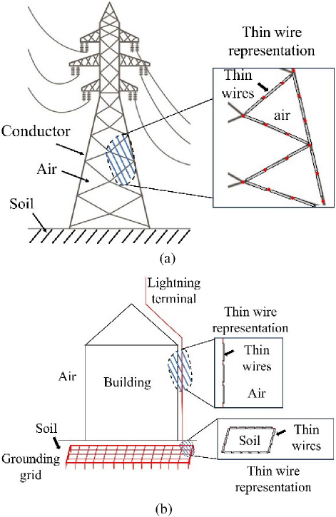
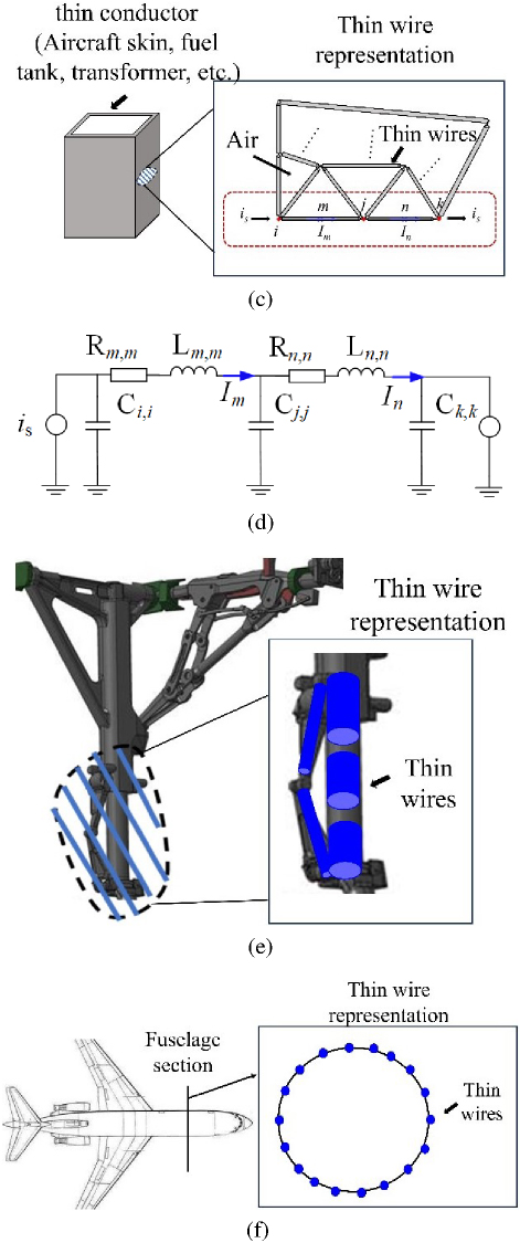
Figure 1: Power PEEC of the thin-wire model. (a) Thin-line representation process of a high-voltage tower [27, 35], (b) thin-wire representation process of a grounding grid [35], (c) structures modeled as thin lines, (d) equivalent circuit diagram of some nodes and sticks, (e) thin-wire representation process of landing gear [30], and (f) thin-wire representation process of aircraft fuselage cross-section [25].

This paper focusses on current distribution inversion, in which surface structures are represented by thin wires, when lightning strikes an aircraft. Unlike the soil medium that exists in a ground lightning strike environment, only one air medium exists when an aircraft is struck by lightning. When the aircraft is discretized using triangular surface elements, the edges of the triangle are extracted as line segments, as shown in Fig. 1 (c). The equivalent circuit model can be obtained according to the PEEC, as shown in Fig. 1 (d).

In Fig. 1 (c), the red dots represent the potential (capacitance) matrix node, which correspond to the potential matrix element C $_{i, i}$ , and the blue crosses represent the inductance (current) matrix node, which corresponds to the resistance matrix element R $_{m, m}$ and inductance matrix element L $_{m, m}$ of the sticks, where the subscripts i, j, and k represent the ith, jth, and kth points, respectively, and m and n represent the mth andnth sticks, respectively. i $_{s}$ represents the injected current of the node.

According to Fig. 1 (d), the PEEC equation can be expressed as:

[\begin{matrix} A^{T} & R + j ω L \\ j ω P^{- 1} + Y_{L} & - A \end{matrix}] [\begin{matrix} V \\ I \end{matrix}] = [\begin{matrix} - Vs \\ Is \end{matrix}],

(1)

The voltages and currents at the grid nodes can be solved by inverting the matrix. To calculate the matrix in equation (2), this study used the Gauss-Legendre quadrature formula [23].

III. SIMPLIFICATION OF PEEC AND THE INVERSION METHOD OF SURFACE CURRENT DISTRIBUTION

A. Simplification of PEEC

In PEEC for surface structures, using a finite number of sticks to represent the conductors may introduce a capacitance that does not exist. To avoid introducing a capacitor, the current flowing through it can be ignored. The PEEC equations can be simplified as:

[\begin{matrix} R + j ω L & A^{T} \\ A & 0 \end{matrix}] [\begin{matrix} I \\ V \end{matrix}] = [\begin{matrix} - Vs \\ - Is \end{matrix}] .

(3)

To analyze the influence of simplification, the results of considering and not considering the capacitor are compared in parts A and B of section IV by sweeping the frequency and injecting the time-domain lightning current, respectively.

Because lightning current is typically expressed as a function of time I(t), fast Fourier transformation (FFT) is required to obtain I( $ω$ ); thus, the current in the frequency domain can be obtained via equation (3). The current in the thin wire ${\vec{I}}_{i}$ in the time-domain can be obtained by performing an inverse FFT (IFFT) on the results. The errors caused by the FFT and IFFT are also analyzed in part C of section IV.

B. Magnetic field calculation method

According to Maxwell’s equations, the magnetic field and vector magnetic potential satisfy the following relationship:

\vec{B} = \nabla \times \vec{A} .

(4)

Thin-line currents can then be used to calculate the vector magnetic potential. The magnetic field intensity at observation point P is generated by all the line currents passing through the following:

$H$	$= \frac{\nabla \times A}{μ_{0}} = \frac{1}{4 π} \sum_{i = 1}^{l} \nabla \times \int_{l_{i}} \frac{{\vec{I}}_{i}}{\| \vec{r_{p}^{'}} - \vec{r_{i}^{'}} \|} d l_{i}$
		$= \frac{1}{4 π} \sum_{i = 1}^{l} \int_{l_{i}} \frac{{\vec{I}}_{i} \times r^{'}}{r^{', 3}} d l_{i}$	(5)

where l $_{i}$ represents the length of the ith line, ${\vec{I}}_{i}$ represents the current vector on the ith line, and $| \vec{r_{p}^{'}} - \vec{r_{i}^{'}} |$ represents the distance between the observation point and differential element. To distinguish it from r, r’ is used to represent the distance between P and the integration position point.

C. Inversion method of the surface current distribution

After obtaining H, J $_{s}$ can be expressed according to the continuity conditions at the interfaces:

J_{s} = e_{n} \times (H_{2} - H_{1}) .

(6)

The surface current density can then be derived from the magnetic field using equation (6). In FDTD or FEM, surface currents are often calculated by interpolating adjacent grids [36]. In the 1D PEEC, only the conductor is meshed, whereas free space is not (as shown in Fig. 1). In this case, the positions of H $_{1}$ and H $_{2}$ cannot be determined and, as a result, J $_{s}$ cannot be estimated using equation (6). The key to estimating J $_{s}$ lies in determining the height of the magnetic field calculation.

To determine the height, ignoring the influence of other strong magnetic field sources, for a current-carrying conductor, the closer the magnetic field observation point is to the current-carrying conductor, the stronger the magnetic field strength.

Based on the assumptions above, the magnetic field at the height at which the maximum magnetic field occurs can be used to estimate J $_{s}$ . However, when the structure is represented by thin wires, the surface element is filled with an air medium, and all thin-line currents generate a magnetic field. Therefore, it may be difficult to determine the height of the peak value of the magnetic field.

The magnetic field strength of all the surface elements is determined by taking the radius of the thin wire as the step size. The height of the magnetic field calculation point is then defined as k times the radius of the conductor, as shown in Fig. 2.

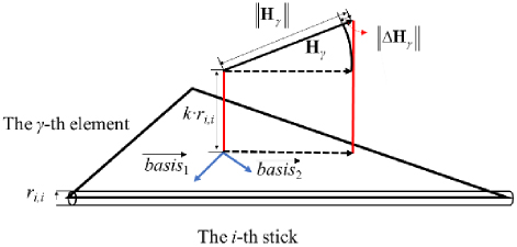
Figure 2: Inversion method of the surface current distribution.

The average value of the magnetic field strength of all surface elements is defined as:

j_{a} (k)

= \frac{\sum_{γ = 1}^{N_{element}} ∥ H_{γ} ∥}{N_{element}} .

(7)

In equation (7), H $_{γ}$ is the magnetic field strength at a height k $\cdot$ r $_{i, i}$ from the $γ$ -th element. When j $_{a}$ (k) is largest, k is defined as k $_{m a x}$ .

Because the normal vector of H $_{γ}$ is caused by the thin-line representation and k $_{m a x}$ $\cdot$ r $_{i, i}$ height, the magnitude of the magnetic field at k $_{m a x}$ is used to estimate the surface current:

J_{γ} = ∥ H_{γ} (k_{\max}) ∥ .

(8)

In equation (8), the modulus of the magnetic field strength is used to calculate the surface current, rather than the tangential component. Therefore, it is necessary to analyze the differences caused by the orthogonal decomposition.

To analyze the difference, a unit orthogonal basis, $\vec{b a s i s_{1}}$ and $\vec{b a s i s_{2}}$ , on the face element can be determined by the vertices of the face element. The direction of the face element is defined as:

\vec{n_{γ}} = \vec{b a s i s_{1}} \times \vec{b a s i s_{2}} .

(9)

$∥ Δ H_{γ} ∥$ represents the difference between the magnetic field modulus and the tangential component:

\begin{matrix} ∥ Δ H_{γ} ∥ = ∥ H_{γ} ∥ - \\ ∥ H_{γ} ∙ \vec{b a s i s_{1}} \cdot \vec{b a s i s_{1}} + H_{γ} ∙ \vec{b a s i s_{2}} \cdot \vec{b a s i s_{2}} ∥ \end{matrix} .

(10)

The subtrahend in equation (10) represents the magnitude of the tangential component of H $_{γ}$ . Thus, the average error caused by the orthogonal decomposition can be expressed as:

E r r o r_{O D} = \frac{\sum_{γ = 1}^{N_{element}} ∥ Δ H_{γ} ∥}{N_{element}} .

(11)

IV. RESULTS AND DISCUSSION

A. Analysis of the influence of P and delay on the results by sweeping frequency

We first analyzed the impact of the potential matrix and delay on the results from a frequency-domain perspective. Then, we analyzed the efficiency and accuracy of different simulation settings under lightning current excitation and compared them with the finite integration technique (FIT).

In the frequency-domain analysis, currents of different frequencies were injected into an aluminum plate with dimensions of 500 $\times$ 250 $\times$ 2 mm. The current inflow and outflow points are shown in Fig. 3 with an injected current value (I $_{i n j e c t}$ ) of 1 A. The structure was automatically divided into triangular surface elements using commercial software, and the vertex coordinates of the surface elements were extracted to form a thin-wire model constructed using triangular vertices. The number of nodes N was 689.

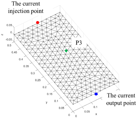
Figure 3: Current outflow and inflow points after flat plate meshing.

As described in part A of section III, the PEEC is simplified by ignoring the capacitance (P). It is necessary to analyze the effect of P on the results. If the capacitance was considered, equation (2) was used. Otherwise, without considering capacitance, equation (3) was used for the solution.

Delay is another factor that influences the results, particularly for large structures. To consider the delay, internal elements P and L in equations (2) and (3) must be modified as follows:

\begin{matrix} P_{d} = P \cdot e^{- j \cdot d \cdot 2 π f \cdot \sqrt{ε_{0} μ_{0}}} \\ L_{d} = L \cdot e^{- j \cdot d \cdot 2 π f \cdot \sqrt{ε_{0} μ_{0}}} \end{matrix} .

(12)

In the above equations, P and L are the matrix elements when the delay is not considered, and P $_{d}$ and L $_{d}$ are the matrix elements when the delay is considered. d in equation (12) is the distance between nodes, f is the frequency of the injected current, and $μ$ $_{0}$ and $ε$ $_{0}$ are the magnetic permeability and dielectric constant in vacuum, respectively. For the specific codes, refer to [36].

The effect of delay on the results was related to the relative size. The relative size is defined as follows:

S = \frac{l_{w}}{l_{p}} = \frac{c}{f \cdot l_{p}},

(13)

where S is the relative size, l $_{w}$ is the wavelength, l $_{p}$ is the physical scale, c is the speed of wave propagation, and f is the frequency.

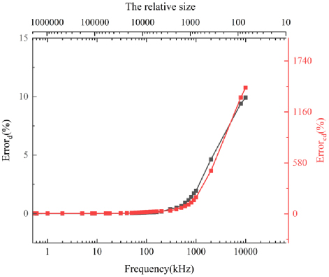
Figure 4: Error at different frequencies. Error $_{d}$ and Error $_{c d}$ calculated by equation (14) represent the differences caused by not considering delay and not considering capacitance and delay, respectively.

Results for different frequencies were compared with those obtained with and without considering P and the time delay, as shown in Fig. 4. The percentage error in Fig. 4 can be expressed as:

e r r o r = \frac{\sqrt{\sum_{j = 1}^{N} {(\hat{i_{j}} - i_{j})}^{2}}}{I_{i n j e c t}} % .

(14)

In equation (14), I $_{i n j e c t}$ is the injected current, which was set to 1 in the situation. N is the total number of current nodes, which was 689. i $_{j}$ is the current of the j-th node when considering capacitance and delay. When calculating the error caused by ignoring delay, $\hat{i_{j}}$ is the j-th node current when delay is ignored and capacitance is considered. When calculating the error caused by ignoring capacitance and delay, $\hat{i_{j}}$ is the node current without considering capacitance and delay.

As shown in Fig. 4, with an increase in the frequency, the error caused by the delay was relatively small at 1 MHz (S $>$ 600, within 2%). It exhibited a rapidly increasing trend after exceeding 1 MHz (S $<$ 600). However, the error was still small, only 9.9% at 10 MHz (S $=$ 60), compared to the results obtained when ignoring P. This is because the aluminum plate analyzed in this study was small.

Ignoring P caused a large difference in the calculation results. The error reached 22% at 100 kHz (S $=$ 6000).

B. Analysis of the influence of P and delay on the results by injecting lightning current component A

The lightning current component A in SAE-ARP-5412 with a duration of 300 μ was sampled at 1 MHz and replaced with the swept frequency current described above. The equation for the lightning current component A is defined as:

I (t) = I_{0} (e^{- α t} - e^{- β t}) {(1 - e^{- γ t})}^{2} .

(15)

In equation (15), I $_{0}$ $=$ 218810, $α$ $=$ 11354, $β$ $=$ 647265, and $γ$ $=$ 5423540. Subsequently, the signal transformed by the FFT was set to inject the current. In Fig. 5 (a), the waveform of lightning current component A is represented by the red curve. Its frequency component is shown in Fig. 5 (b). As shown in Fig. 5 (a), the coordinates of the observation point position P3 were (0.125, 0.250, 0.050) [unit: m].

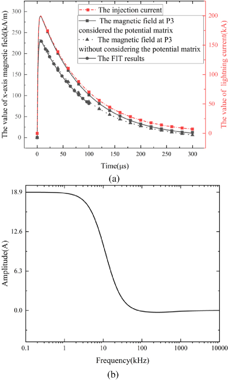
Figure 5: Injected lightning current waveform and magnetic field waveform at the observation point. (a) Magnetic field waveform at position P3 and the injected current and (b) frequency component of lightning current component A.

As shown in Fig. 5 (b), in terms of the frequency components of the lightning current component A, most of the frequency components were within 10 kHz. Therefore, errors caused by P may still be extremely small.

As shown in Fig. 5 (a), the results when the potential matrix was considered were higher than those when the potential matrix was not considered. The error between the two values was within 18%. Moreover, as the waveform slowed down, the error caused by P gradually decreased, which was caused by $ω$ in PEEC (see equation (1)). If $ω$ is small, $j ω P^{- 1}$ is small and $j ω P^{- 1} + Y_{L}$ can be set to 0. Then, equations (1) and (3) are equivalent.

From the frequency perspective, the trailing edge of the lightning current waveform corresponded to the low-frequency region, and the error in the low-frequency region was relatively low, as shown in Fig. 4.

In any case, the error at the peak moment in the time domain was considerably lower than that shown in Fig. 4 because the lightning current component A had greater energy at low frequencies.

As shown in Fig. 5 (a), the high amplitude of the magnetic field caused by P can be explained in two ways. First, in the EFIE, the scalar potential term causes the electric field to increase, which leads to an increase in the thin-line current in the solution. Second, the addition of a potential matrix considers the current in the capacitor branch. The current in the capacitor increases the amplitude of the thin-line current when it flows into the node.

However, before the actual non-thin wire conductive structure was meshed, the inside of the structure was not filled with air. The capacitance term in PEEC could not be introduced at this time. By comparing the results of PEEC and FIT, it was found that the consistency between the FIT and PEEC was higher when the capacitance term was not considered. At this point, P caused the magnetic field calculation results to be too large.

Table 1: Simulation settings and time consumption

Method	Number of Sticks	Number of Nodes	Sampling Frequency (MHz)	Time of Waveform ( $μ$ s)	Time (s)
Method 1	45	20	2	100	0.089338
Method 2	689	250	2	100	11.745
Method 3	4597	1584	2	100	1158.3
Method 4	689	250	10	300	176.47
Method 5	689	250	100	300	1818.31
Method 6	689	250	10	500	301.3620255
Method 7	689	250	500	100	3002.46
Method 8	689	250	2	500	57.7893795
	Number of Cells		Frequency Range (MHz)	Time of Waveform ( $μ$ s)
FIT	38080		0 $\sim$ 100	100	2 h 58 min

Table 2: Simulation results of different methods

Method	Peak Value of Magnetic Field Intensity of X-Axis (Ka/M)
	P1	P2	P3	P4	P5
Method 1	239.06	247.63	236.39	235.76	231.37
Method 2	239.30	240.98	236.59	241.23	238.46
Method 3	238.32	238.24	233.69	238.25	238.31
Method 4	239.46	241.18	236.79	241.43	238.62
Method 5	239.46	241.18	236.79	241.43	238.62
Method 6	239.5	241.26	236.88	241.52	238.68
Method 7	239.27	240.95	236.55	241.19	238.44
Method 8	239.52	241.25	236.87	241.50	238.67
FIT	237.9	238.4	230.9	238.4	237.9

C. Analysis of the influence of FFT and mesh density on the results

Because the accuracy of the results highly depends on the mesh density and FFT operations, the influence of the related settings of the mesh density and FFT should be analyzed.

Simulation settings are listed in Table 1. Methods 1-3 were used to compare the impact of the mesh density on the results. In addition, Methods 4-8, which involved changing the sampling frequency and duration of the source, were used to compare the impact of FFT on the results.

In the simulation, five observation points were selected to analyze the amplitude of the results. The coordinates of these points were P1 (0.075, 0.250, 0.050), P2 (0.125, 0.150, 0.050), P3 (0.125, 0.250, 0.050), P4 (0.125, 0.350, 0.050), and P5 (0.175, 0.250, 0.050) (unit: m). The results for these five points are listed in Table 2. Because P3 is above the center of the plate, P1 and P2 are symmetrical, and P4 and P5 are symmetrical. The x-axis magnetic fields at P1, P2, P4, and P5 should be equal.

Under different mesh densities (Methods 1-3), this feature became more evident as the number of thin lines increased. In Method 3, the difference in the magnetic fields between the two pairs of symmetrical positions was considerably smaller than that of the FIT, which indirectly verified the accuracy of the results. At the same time, when comparing Methods 4-8, changes in the sampling frequency and waveform duration did not cause major changes in the results.

In addition to amplitude comparison, the magnetic field at the center point was compared, as shown in Fig. 6. Because the time-domain waveforms under different simulation settings were not very different, we compared the single-sided frequency spectra of the results in Fig. 6 (a), as shown in Fig. 6 (b).

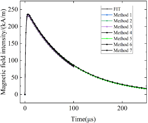
Figure 6: Results of the FIT and PEEC methods. (a) Time-domain waveforms obtained using different methods and (b) frequency-domain waveforms obtained using different methods.

Comparing the results of Methods 1-3 in Fig. 6 (b), the power spectra of different mesh densities were consistent. The duration of the excitation source and the sampling frequency affected the spectrum.

The effect of the duration on the result was small, as in Methods 4 and 6 in Fig. 6 (b). The reason for the small difference is that the FFT of the nonperiodic signal was obtained by extending the signal after truncation, and lightning current component A had less energy after 300 μ.

The sampling frequency had a greater impact on the spectrum than on the waveform time, as in Methods 4 and 5. As the sampling frequency increased, the spectrum gradually became consistent with that of the FIT. Although there were certain differences in the frequency domains between the different frequency methods, Table 2 and Fig. 6 (a) show that the peak value and time-domain waveform of the magnetic field were not significantly different. Therefore, the magnetic field results obtained using the simplified PEEC equation were accurate. In addition, the results indicated that the relevant settings and solution results of the entire FFT and IFFT processes were reliable.

From the perspective of computational time, the thin-line model under the PEEC method was considerably faster than that under the FIT. As shown in Table 1, the grid became denser and the calculation time increased; however, the time was significantly less than that taken by the FIT. Therefore, the line-network model was more efficient.

D. Surface current distribution

Next, the method for estimating the surface current distribution was verified by comparing it with the FIT. The average error caused by orthogonal decomposition (Error $_{O D}$ ) was also analyzed.

The Error $_{O D}$ values calculated using equation (11) and the average current density j $_{a}$ (k) of the surface element calculated using equation (7) at different k values at 6 μ are shown in Fig. 7.

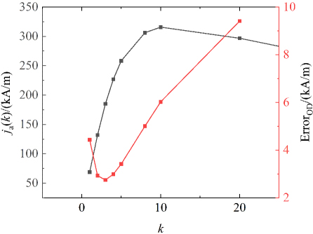
Figure 7: Results of Error $_{O D}$ and j $_{a}$ (k) at different heights.

Figure 7 shows the average current density on the surface elements, which first increased and then decreased with increasing height. The maximum surface current was observed when k reached approximately 10 (at a height of approximately 10 mm). Error $_{O D}$ first decreased and then increased with height, reaching a minimum value when k was approximately 3 (at a height of approximately 3 mm). The normal magnetic field component of the panel near this position was thesmallest.

As shown in section III, the magnitude of the magnetic field at k $_{m a x}$ can be used to estimate the surface current rather than the tangential component and minimum height of Error $_{O D}$ . We explain the reason for this estimation by presenting the results of the surface current distribution in Fig. 8. Surface currents were calculated using k $=$ 10 and k $=$ 3. FIT results were used for comparison, as shown in Fig. 9. Moreover, the maximum and minimum values of the color bars are kept consistent in Figs. 8 and 9.

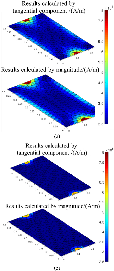
Figure 8: Results of the current distribution. (a) Surface current distribution at k $=$ 10. The height of the magnetic field calculation point for each surface element is 10 mm. (b) Surface current distribution at k $=$ 3. The height of the magnetic field calculation point for each surface element is 3 mm.

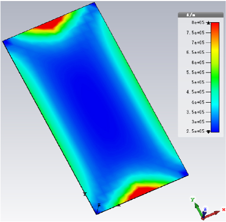
Figure 9: FIT results of the lightning current distribution of the plate at 6 μ.

As shown in Fig. 9, the lightning current flowed along the edges. In addition, results indicate that the current flowing through the edge was approximately 4.5 $\times$ 10 $^{5}$ A/m. The currents at the injection and outflow points exceeded 8 $\times$ 10 $^{5}$ A/m.

As shown in Fig. 8 (a), the tangential component may not be suitable for inverting the surface current distribution. Orthogonal decomposition of the plate-edge magnetic field would result in loss of the magnetic field in the normal direction, decreasing the current density on the edge surface.

When k $=$ 3, Error $_{O D}$ was the smallest, the surface current at the injection point was greater than 6 $\times$ 10 $^{5}$ A/m, and the edge surface current density was approximately 3 $\times$ 10 $^{5}$ A/m, as shown in Fig. 8 (b). However, the estimated results for the surface current were too small, which indicates that the minimum height of Error $_{O D}$ cannot be used to reflect the surface current distribution.

When k $=$ 10, j $_{a}$ (k) was largest, and the inversion results of the thin-wire model were closer to the FIT results. Therefore, FIT verified that the surface current density could be effectively inverted by determining the height with the maximum average current density.

According to the above analysis, the thin-line model did not exhibit a stronger magnetic field closer to the observation point of the current-carrying structure. Instead, as the distance decreased, it showed a trend of first increasing and then decreasing, as shown in Fig. 7.

E. Current distribution inversion for a real case

In part D, an inversion method for the surface current distribution of the thin-line model is introduced. Although a flat plate is the basic unit of complex structures, there are many structures with large curvatures, such as aircraft wings and vertical tails. Therefore, lightning current distribution in an elliptical barrel was analyzed.

The long semi-axis of the elliptical barrel was 90 mm, the short semi-axis was 45 mm, and its length was 1.2 m. The lightning current was injected through four points and flowed out from four points, as shown in Fig. 10. The lightning current component A injected into the structure was 200 kA. Therefore, the current injected at each point was set as 50 kA.

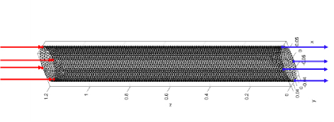
Figure 10: Schematic diagram of elliptical barrel lightning current injection.

Table 3: Simulation results of different methods

Method	Number of Sticks	Number of Nodes	Sampling Frequency (MHz)	Time of Waveform ( $μ s$ )	Calculation Time/s	Inversion Time (s)
						Without Using Parallel Computing	Using Parallel Computing
PEEC	15970	5350	1	100	14653	26481	4074
Number of Cells	Frequency Range (MHz)	Calculation Time (s)
FIT	63648	0 100	72534

The number of sticks and nodes and the calculation time for the elliptical barrel after being represented by a thin line are listed in Table 3. To avoid meshing the 1-mm-thick structure, the elliptical barrel was modeled as a 1-mm-thick surface. If the mesh step size was too small, the calculation time was very long.

According to Table 3, when the number of sticks and nodes was large, that is, when the number of surface elements was large, the inversion time was longer, which is equivalent to the calculation time. This is because the inversion process of every surface element must calculate the contribution of all line currents. The calculations of the current distribution for each element were independent of each other. Therefore, parallel computing technology was introduced with 12 workers, and the time required to invert the panel current was reduced sharply from 26481 to 4074 s.

The representation of the physical structure using the thin-wire model fixes the flow direction of the current, which may be one of the reasons for its high computational efficiency. Based on these comparisons, the use of PEEC under the thin-line model was more efficient than the use of FIT. This is possibly because magnetic field and surface current distribution of the entire calculation space were not obtained, unlike in FIT. Subsequently, magnetic field and surface current distribution results were obtained by post-processing the results. For complex models, the inversion time may be extremely long; however, as shown in Table 3, the inversion efficiency can be improved through parallel computing.

In addition, the surface current distribution at 6 μ is shown in Figs. 11 (a) and (b), and the Error $_{O D}$ calculated using equation (11) and the average current density j $_{a}$ (k) calculated using equation (7) at different k values at 6 μ of the elliptical barrel are shown in Fig. 11 (c).

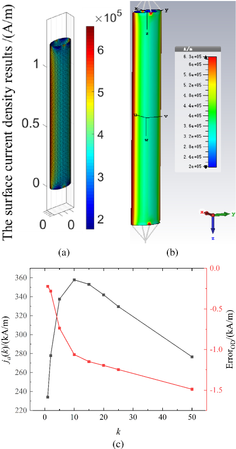
Figure 11: Lightning current distribution results for the elliptical barrel: (a) PEEC results, (b) FIT results, and (c) Error $_{O D}$ and j $_{a}$ (k) at different heights in the elliptical barrel case.

Figure 11 shows that even for a structure with a certain curvature, such as an ellipse, the surface current distribution obtained by the inversion method in this study was highly consistent with FIT. In addition, as shown in Fig. 11 (c), even when the model and structure thicknesses changed, the magnetic field calculation point position remained near k $=$ 10. The error caused by orthogonal decomposition was different from that shown in Fig. 7 and continued to increase.

V. DUAL CHARACTERISTIC ANALYSIS UNDER THE PEEC FRAMEWORK

In sections III and IV, the PEEC equation is simplified by ignoring P, and surface current distribution inversion is discussed. For high frequencies and certain situations where electric field effects are considered, such as electromagnetic wave scattering and HIRF problems, it is necessary to consider the potential matrix. For some complex structures, nonsparse P and L matrices often require large amounts of memory storage and calculation processes.

Although Darney et al. analyzed the P and L characteristics of a 2D cross-section [21], the equation in three-dimensional (3D) space was not given. Therefore, the equation for the 3D thin lines was derived as follows:

\begin{matrix} L_{i, j} \cdot C_{i, j} & = & L_{i, j} / p_{i, j} \end{matrix} .

(16)

However, equation (16) is not completely equal and cannot be established even at certain positions.

For some edge points, the length of the sticks when calculating the potential node was inconsistent with the length of the inductance sticks, such as the starting point of a long straight wire. Second, because the inductance matrix is defined based on sticks, its dimensions are l $\times$ l, whereas the potential matrix is defined based on nodes, and its dimensions are n $\times$ n. For a set of L $_{i}$ $_{,}$ $_{j}$ and C $_{i}$ $_{,}$ $_{j}$ with the same subscript, there may be no correspondence between the points and lines.

Simple mathematical operations were performed on the above equation to present it in graphical form:

\frac{L_{i, j} \cdot C_{i, j}}{μ_{0} \cdot μ_{r} \cdot ε_{0} \cdot ε_{r} \cdot < \vec{l_{i}}, \vec{l_{j}} >} \approx 1 .

(17)

In particular, when l $_{i}$ and l $_{j}$ are perpendicular, the denominator of the above equation is zero and the equation does not hold.

To verify equation (17), a finite-length straight wire was used as a simple example. The wire was divided into several segments. The first 10 rows and first 10 columns of the P and L matrices were substituted into the above formula, and the results were compared when the numbers of Gaussian calculation points were different, as shown in Fig. 12.

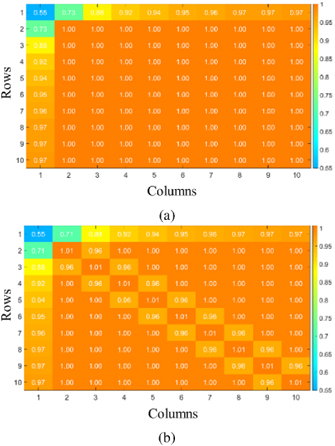
Figure 12: Relationship between the P and L matrices: (a) number of Gaussian calculation points is 100 and (b) number of Gaussian calculation points is 2.

Because P and L are symmetric matrices, and the nodes and sticks correspond exactly for long straight wires, the matrix shown in Fig. 12 was also symmetric. In addition, Gaussian calculations for the number of points can strengthen the relationship in equation (17). This is because the calculation results became more accurate as the number of calculation points increased. For Row 1 and Column 1, the addition of Gaussian calculation points did not significantly change the results. In addition, the first point in Row 1 and Column 1 did not satisfy equation (17). This is because P $_{1, 1}$ or C $_{1, 1}$ is an isolated point. When the point is calculated, it is only half the integral pathof len $_{1}$ .

In addition, the matrix elements of the first 10 rows and columns of the P and L matrices in Method 2 shown in part B of section IV and in the literature [36] were compared. The plate in [36] was divided into a rectangular grid using equation (17), and the calculation results are shown in Fig. 13.

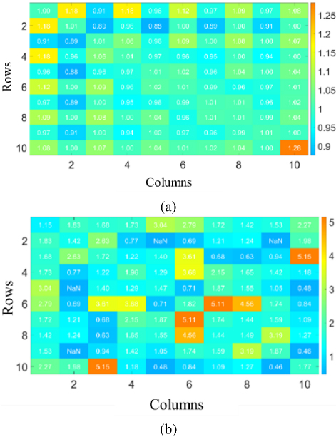
Figure 13: Relationship between the P and L matrices of different grids: (a) rectangular grid and (b) triangular grid.

The rectangular mesh had more positions that complied with equation (17) because there were more finite-length straight-wire structures [36]. Compared to rectangular grids, triangular grids had fewer positions that satisfy equation (17). This is because a set of L $_{i, j}$ and C $_{i, j}$ with the same subscript mentioned above may not correspond to nodes and sticks. In addition, the NaN symbol in Fig. 13 indicates that the angle between l $_{i}$ and l $_{j}$ was 90 $^{\circ}$ .

The P-L relationship may help researchers understand the relationship between P and L while reducing memory storage. Because the matrix constructed using equation (17) has a large number, 1, as shown in Fig. 12, it is only necessary to construct a dense P or L and construct a sparse P-L relationship matrix by setting 1 to 0 in the matrix, thereby establishing another dense matrix based on the sparse P-L relationship matrix. This operation can reduce the storage space of a dense matrix, thereby improving its performance.

VI. CONCLUSION

To address the question of lightning current distribution when a non-thin wire structure is equivalent to a thin-line model, this study developed the PEEC method and performed it in the frequency domain. A magnetic field calculation equation was derived, which is more convenient for experimental verification. An inversion method for the surface current density was then established. In addition, parallel computing technology was used to increase inversion efficiency. The method in this study is extremely efficient and can be extended to simulate lightning current distribution in complex structures. The accuracy of the results was close to that of the FIT. The main conclusions are as follows.

(1) Calculation efficiency of the thin-line model was considerably greater than that of the FIT. For flat and elliptical structures, the calculation results were highly consistent with those of the FIT.

(2) Influence of time delay and potential matrix on the solution results was analyzed. It was found that these influences depended on the frequency. The error gradually increased with an increase in frequency. When the scale of the problem was within $S = 60$ , the error caused by the time delay was within 10%. Although there was a large difference in the results caused by the potential matrix, the results obtained by ignoring the potential matrix for non-thin conductor structures were more accurate when compared with the FIT.

(3) Surface current density of the thin-line model was effectively obtained by inverting the surface current through the maximum magnetic field position.

(4) For the thin-line model, as the height increased, the magnetic field first increased and then decreased. Even when the height was approximately 10 times the radius of the thin sticks, the magnetic field intensity was maximized for a flat plate or ellipticalbarrel.

ACKNOWLEDGMENTS

This study was supported by the National Key Laboratory of Electromagnetic Information Control and Effects (grant number 20240404 MJZ5-2N22 and 50909030401). We would like to thank the reviewers for their professional comments, which helped us improve the quality of the manuscript, as well as the editors.

REFERENCES

[1] Roger F. Harrington, Field Computation by Moment Methods. Oxford: Oxford University Press, 1996.

[2] J.-M. Jin, The Finite Element Method in Electromagnetics. Hoboken, NJ: John Wiley & Sons, 2015.

[3] T. Weiland, “A discretization model for the solution of Maxwell’s equations for six-component fields,” Archiv Elektronik und Uebertragungstechnik, vol. 31, pp. 116-120, Apr. 1977.

[4] A. E. Ruehli, “Inductance calculations in a complex integrated circuit environment,” IBM Journal of Research and Development, vol. 16, no. 5, pp. 470-481, 1972.

[5] Y. Kane, “Numerical solution of initial boundary value problems involving Maxwell’s equations in isotropic media,” IEEE Transactions on Antennas and Propagation, vol. 14, no. 3, pp. 302-307, 1966.

[6] C. Tong, S. Qiu, X. Si, Z. Duan, Z. Li, and Y. Li, “Research on the lightning current distribution simulation and lightning test of a passenger aircraft’s vertical tail,” Fiber Composites, vol. 3, p. 5, 2021.

[7] K. Sun, X. Zhao, G. Zhang, and H. Zhang, “Numerical simulations of the lightning attachment points on airplane based on the fractal theory,” Acta Phys. Sin., vol. 63, no. 2, pp. 1-7, 2014.

[8] J. Yang, X. Qie, J. Wang, Y. Zhao, Q. Zhang, T. Yuan, Y. Zhou, and G. Feng, “Observation of the lightning induced voltage in the horizontal conductor and its simulation,” Acta Phys. Sin., vol. 57, p. 8, 2008.

[9] G. A. Rasek and S. E. Loos, “Correlation of direct current injection (DCI) and free-field illumination for HIRF Certification,” IEEE Transactions on Electromagnetic Compatibility, vol. 50, no. 3, pp. 499-503, 2008.

[10] Y. Liu, Z. Fu, A. Jiang, Q. Liu, and B. Liu, “FDTD analysis of the effects of indirect lightning on large floating roof oil tanks,” Electric Power Systems Research, vol. 139, pp. 81-86, 2016.

[11] M. R. Alemi, S. H. H. Sadeghi, and H. Askarian-Abyaneh, “A marching-on-in-time method of moments for transient modeling of a vertical electrode buried in a lossy medium,” IEEE Transactions on Electromagnetic Compatibility, vol. 64, no. 6, pp. 2170-2178, 2022.

[12] C. Tong, Z. Duan, Y. Huang, S. Qiu, X. Si, Z. Li, and Z. Yuan, “Study of the B-dot sensor for aircraft surface current measurement,” Sensors, vol. 22, no. 19, p. 7499, 2022.

[13] G. Gutiérrez, R. M. Castejón, H. Tavares, H. Galindo, E. P. Gil, M. R. Cabello, and S. G. García, “Validation of lightning simulation compared with measurements using DCI technique post-processed to be applied to a lightning threat,” IEEE Transactions on Electromagnetic Compatibility, vol. 65, no. 1, pp. 281-291, 2023.

[14] K. S. H. Lee, EMP Interaction: Principles, Techniques, and Reference Data: A Handbook of Technology from the EMP Interaction Notes. London: Hemisphere Publishing Corporation,1986.

[15] R. Mittra, Numerical and Asymptotic Techniques in Electromagnetics. New York: Springer, 1975.

[16] G. E. Bridges and L. Shafai, “Validity of the thin-wire approximation for conductors near a material half-space,” Digest on Antennas and Propagation Society International Symposium, pp. 232-235, 1989.

[17] T. Bauernfeind, P. Baumgartner, O. Bíró, A. Hackl, C. Magele, W. Renhart, and R. Torchio, “Multi-objective synthesis of NFC-transponder systems based on PEEC method,” IEEE Transactions on Magnetics, vol. 54, no. 3, pp. 1-4, 2018.

[18] P. Baumgartner, T. Bauernfeind, O. Bíró, A. Hackl, C. Magele, W. Renhart, and R. Torchio, “Multi-objective optimization of Yagi-Uda antenna applying enhanced firefly algorithm with adaptive cost function,” IEEE Transactions on Magnetics, vol. 54, no. 3, pp. 1-4, 2018.

[19] R. Torchio, P. Alotto, P. Bettini, D. Voltolina, and F. Moro, “A 3-D PEEC formulation based on the cell method for full-wave analyses with conductive, dielectric, and magnetic media,” IEEE Transactions on Magnetics, vol. 54, no. 3, pp. 1-4, 2018.

[20] G. Antonini, A. E. Ruehli, D. Romano, and F. Loreto, “The partial elements equivalent circuit method: The state of the art,” IEEE Transactions on Electromagnetic Compatibility, vol. 65, no. 6, pp. 1695-1714, 2023.

[21] I. B. Darney, Circuit Modelling for Electromagnetic Compatibility. Raleigh, NC: Scitech Publishing, pp. 15-20, 2013.

[22] I. B. Darney, “Grounding, floating and screening,” in IET Conference Proceedings, London, UK, 2000.

[23] R. Torchio, “PEEC modelling of large-scale fusion reactor magnets,” thesis, Universita’ Degli Studi Di Padova, 2016.

[24] I. B. Darney and C. M. Hewitt, Darney’s Circuit Theory and Modelling: Updated and Extended for EMC/EMI. Raleigh, NC: Scitech Publishing, 2023.

[25] J. Parmantier, F. Issac, and V. Gobin, “Indirect effects of lightning on aircraft and rotorcraft,” Journal Aerospace Lab., vol. 5, no. 5, pp. 1-27, 2012.

[26] W. Ye, W. Liu, N. Xiang, K. Li, and W. Chen, “Analytical evaluation of partial elements in the full-wave PEEC formulation for thin-wire structure,” IEEE Transactions on Electromagnetic Compatibility, vol. 65, no. 5, pp. 1410-1421, 2023.

[27] W. Ye, W. Liu, N. Xiang, K. Li, and W. Chen, “A full-wave PEEC model for thin-wire structure in the air and homogeneous lossy ground,” IEEE Transactions on Electromagnetic Compatibility, vol. 65, no. 2, pp. 518-527, 2023.

[28] W. Ye, W. Liu, N. Xiang, K. Li, L. Cheng, B. Hu, Y. Zhou, and W. Chen, “A low-frequency approximation PEEC model for thin-wire grounding systems in half-space,” IEEE Transactions on Power Delivery, vol. 38, no. 2, pp. 1297-1307, 2023.

[29] B. Li, Z. Du, Y. Du, Y Ding, Y Zhang, J. Cao, L. Zhao, and J. Chen, “An advanced wire-mesh model with the three-dimensional FDTD method for transient analysis,” IEEE Transactions on Electromagnetic Compatibility, pp. 1-10, 2023.

[30] D. Prost, F. Issac, T. Volpert, W. Quenum, and J. P. Parmantier, “Lightning-induced current simulation using RL equivalent circuit: Application to an aircraft subsystem design,” IEEE Transactions on Electromagnetic Compatibility, vol. 55, no. 2, pp. 378-384, 2013.

[31] Yinghua Lv, Numerical Methods for Computing Electromagnetism. Beijing: Tsinghua University Press, 2006.

[32] R. Torchio, P. Bettini, and P. Alotto, “PEEC-based analysis of complex fusion magnets during fast voltage transients with H-matrix compression,” IEEE Transactions on Magnetics, vol. 53, no. 6, pp. 1-4, 2017.

[33] Z. Xiongfei, B. Shirong, L. Zhengxiang, N. Junsong, Z. Cheng, and C. Liu, “FDTD calculation of the current distribution of microstrip transmission line circuits,” in 2012 International Conference on Computational Problem-Solving (ICCP), Leshan, pp. 245-247, 2012.

[34] J. Cao, Y. Du, Y. Ding, B. Li, R. Qi, Y. Zhang, and Z. Li, “Lightning surge analysis of transmission line towers with a hybrid FDTD-PEEC method,” IEEE Transactions on Power Delivery, vol. 37, no. 2, pp. 1275-1284, 2022.

[35] Y. Zhang, H. Chen, Y. Du, Z. Li, and Y. Wu, “Lightning transient analysis of main and submain circuits in commercial buildings using PEEC method,” IEEE Transactions on Industry Applications, vol. 56, no. 1, pp. 106-116, Jan.-Feb. 2020.

[36] https://github.com/UniPD-DII-ETCOMP/PEEC-1D

BIOGRAPHIES

Zemin Duan was born in Hefei, China, in 1955. He received a B.Sc. from Hefei University of Technology in 1982, and M.Sc. and Ph.D. from the Institute of Plasma Physics, Chinese Academy of Sciences, in 1990 and 1994, respectively. He is a professor at the School of Electrical Engineering, Hefei University of Technology, Chief Specialist of the AVIC Technology Foundation Establishment in Lightning Protection of Airplanes, member of the National Technical Committee for Standardization of Lightning Protection, China, and member of AAAF and SAE. He has been engaged in professional research on pulse power technology and lightning protection of aircraft for more than 20 years.

Chen Tong was born in Yangzhou, Jiangsu, China, in 1995. He received a B.S. in engineering from Hunan Institute of Technology in 2018. Since 2018, he has been studying for a doctorate at the School of Electrical Engineering and Automation, Hefei University of Technology. From 2019 to 2023, he was engaged in research related to aircraft lightning protection and surface lightning current calculation and measurement.

Yeyuan Huang was born in Hefei, Anhui, China, in 1989. He received a B.S. from Anhui University of Science and Technology. He received a Ph.D. from University of Science and Technology of China in 2021. From 2022 to 2023, he worked at the Anhui Provincial Key Laboratory of Aircraft Lightning Protection and the Aerospace Science and Technology Key Laboratory of Strong Electromagnetic Environment Protection Technology. During this time, he conducted research related to the protection of aircraft from high-intensity radiation fields.

Xinping Li was born in Ningyuan County, Hunan Province, in 1980. He received a Bachelor of Science degree in Mathematics and Applied Mathematics from Hunan Institute of Technology in 2004, a Master of Science degree in Probability Theory and Mathematical Statistics from Central South University in 2012, and a Master of Science degree in Computational Mathematics from Hunan University in 2021. Doctor of Science degree. He has been working in the School of Mathematics of Hunan University of Technology since 2004. He was hired as a lecturer in 2010 and an associate professor in 2023. He has published in IEEE Geoscience and Remote Sensing Letters, Remote Sensing, Journal of Computational Physics, Journal of Function Space, Applied Mathematics Letters, and Statistics & Probability Letters. Li is a director of the Hunan Provincial Operations Research Society and a member of the Chinese Society of Industrial and Applied Mathematics.

Shanliang Qiu was born in Hefei, Anhui, China, in 1983. He received the B.S. degree from Hefei University of Technology in 2005. In 2010, he received his Ph.D. from University of Science and Technology of China. He has been working at Anhui Provincial Key Laboratory of Aircraft Lightning Protection and Aerospace Science and Technology Key Laboratory of Strong Electromagnetic Environment Protection Technology since 2011. In the laboratory, he is mainly engaged in aircraft electrostatic discharge brushes and aircraft deposition electrostatic protection related work.

Xiaoliang Si was born in 1985 in Changchun, Jilin Province. He is a Ph.D. and an associate researcher. His main research direction is the strong electromagnetic environment protection technology for aircraft.

Yan Wei is currently studying for his Ph.D. in the Lightning Protection Laboratory of Aircraft at Hefei University of Technology. His main research interests are lightning discharge and electrostatic electromagnetic environmental effects. He is engaged in aircraft electrostatic discharge brushes and aircraft deposition electrostatic protection related work.

Yao Ling was born in Anqing, Anhui, China, in 1996. She received a B.S. in engineering from Qingdao University of Science and Technology in 2018. Since 2018, she has been studying for a doctorate in School of Electrical Engineering and Automation, Hefei University of Technology. From 2019 to 2023, she has been engaged in research related to aircraft lightning protection.