Advanced Physical Optics-inspired Support Vector Regression for Efficient Modeling of Target RCS

Chenge Shi${}^{\mathbf{\text{1}}}$, Rui Cai${}^{\mathbf{\text{1}}}$, Wei Dong${}^{\mathbf{\text{1}}}$, and Donghai Xiao${}^{\mathbf{\text{2}}}$

¹AVIC Xi’an Aircraft Industry Group Company Ltd.
Xi’an, Shaanxi 710089, China
Chen_geShi7@126.com, cairui1201@126.com, 983683251@qq.com

²Xidian University
Xi’an, Shaanxi 710071, China
xiaodonghai@xidian.edu.cn

Submitted On: December 9, 2024; Accepted On: April 17, 2025

ABSTRACT

This paper proposes an advanced physical optics-inspired support vector regression (APOI-SVR) for efficiently modeling the radar cross section (RCS) of conducting targets. Specifically, an improved physical optics-inspired kernel function is newly proposed by introducing two angular frequency parameters, thereby enhancing the capability of characterizing the various fluctuation patterns in RCS with respect to observation angles. Furthermore, considering the critical role of data preprocessing in facilitating the model’s ability to learn the underlying RCS patterns accurately, a physics-based data preprocessing method is introduced. Numerical validations based on two exemplary targets demonstrate that APOI-SVR effectively reduces the predictive root mean square error (RMSE) by over 24.7% compared with the benchmark model. Afterward, APOI-SVR is adopted to quickly establish the RCS feature map of an aircraft model, the results show that it is comparable to numerical simulations in accuracy but less than one-tenth in time cost, indicating the practicality of APOI-SVR for efficiently analyzing the RCS characteristics of targets.

Index Terms: Angular frequency parameter, data preprocessing, physical optics, radar cross section, support vector regression.

I. INTRODUCTION

In the domain of electromagnetic scattering research, the accurate prediction of the radar cross section (RCS) of a target is essential for target recognition and tracking [1, 2], and also exerts a profound influence on a variety of modern applications across aerospace and civilian domains [3–5]. Computational electromagnetic (CEM) methods, such as the finite element method (FEM) [6, 7] and the finite difference time domain (FDTD) [8, 9], have demonstrated remarkable accuracy in simulating the interactions between electromagnetic waves and objects. However, when tasked with modeling complex and electrically-large targets, these methods encounter significant challenges such as the high computational resource demands and extensive time costs for matrix inversion $O(N^3)$, thereby revealing notable limitations in practical application. Researchers have been exploring methods to surmount these computational challenges, such as developing domain decomposition algorithms and acceleration techniques leveraging multi-CPU/GPU architectures [10–12]. These efforts have led to some improvements, but do not constitute a definitive solution. Innovative and potential solutions are still a pressing need to be explored.

In recent years, the rapid advancement of machine learning (ML) has introduced many innovative technical approaches for the modeling and analysis of target’s RCS. For instance, artificial neural networks (ANNs) have been effectively utilized for the real-time prediction of 2D scattered fields [13] and the efficient computation of broadband monostatic RCS of morphing S-shaped cavities [14]. In addition, a hybrid model combining the autoregressive integrated moving average algorithm and the long short-term memory (LSTM) algorithm has been employed for the RCS sequence prediction [15]. Although these methods can model complex nonlinear relationships, they often require a large amount of data for training and can be prone to overfitting on small datasets.

Support vector regression (SVR), a robust machine learning model known for its exceptional nonlinear representation and generalization capabilities, and is less prone to overfitting on small datasets [16–18], has been increasingly incorporated into the field of CEM. Examples include modeling the target’s RCS [19, 20] and the backscattering coefficient of the 3D sea surface [21]. To improve the RCS prediction accuracy of SVR, a physical optics-inspired (POI) kernel function, which is a composite kernel function composed of the cosine function and the Gaussian kernel function, has been proposed [22]. Besides, a comprehensive analysis of the impact of various sampling schemes on the modeling of RCS using the POI kernel-based SVR (termed POI-SVR) has also been conducted. Results show that, compared to the centrally-located sampling (CLS), simple random sampling (SRS), and Latin hypercube sampling (LHS), uniform design (UD) and uniform design sampling (UDS) yield more representative training datasets, which can further improve the RCS modeling precision of POI-SVR. However, the cosine components in the POI kernel function are fixed without adjustable parameters, which limits the ability of POI-SVR to characterize the local fluctuation patterns of RCS. Moreover, the impact of data preprocessing on the modeling accuracy of SVR has not been explored yet.

In this paper, we introduce two angular frequency parameters into the cosine components of the POI kernel function, thereby augmenting the capacity of POI-SVR to characterize the local fluctuation characteristics of the target’s RCS. Also, a physics-based data preprocessing method is proposed to further improve the accuracy of SVR in the modeling of the target’s RCS. To facilitate the follow-up comparative analyses, the advanced POI-SVR presented herein is abbreviated asAPOI-SVR.

The rest of this paper is organized as follows. Section II introduces the proposed APOI-SVR, including the improved POI kernel function, the physics-based data preprocessing method, and the training procedure of APOI-SVR. Several numerical validations for the proposed APOI-SVR are presented in section III. Finally, the conclusion is summarized in section IV.

II. THE PROPOSED APOI-SVR

APOI-SVR mainly improves the kernel function and the data preprocessing method on the basis of POI-SVR. Therefore, in this section, a detailed introduction is mainly given to the improved POI kernel function and the proposed data preprocessing method. The procedure of training APOI-SVR is illustrated at the end of this section as well.

A. Improved POI kernel

It is well accepted that kernel function is crucial for the performance of SVR. For linear problems, a linear kernel function is typically used; for periodic or quasi-periodic issues, a periodic kernel function is often chosen; and to enhance the local representation capability of SVR, a Gaussian kernel function is frequently selected. However, when it comes to complex problems, such as predicting the RCS of complex targets, a suitable kernel function needs to be carefully designed, which demands a deep understanding of the problem (i.e., prior knowledge).

In [22], the backscattered electric field ${\mathit{\text{E}}}_{\mathrm{sca}}(\theta ,\phi ,r)$ is approximated by:

	${\mathit{\text{E}}}_{\text{sca}}(\theta ,\phi ,r)=\mathrm{j}k\eta {\displaystyle \frac{\exp (-jkr)}{4\pi r}}$
	$\mathrm{\hspace{1em}\hspace{1em}}\times {\displaystyle \sum _{i=1}^N}{A}_i\left[\widehat{\mathit{\text{k}}}\times (\widehat{\mathit{\text{k}}}\times {\mathit{\text{J}}}_i^{\prime })\right]\exp [-\mathrm{j2}\mathit{\text{k}}\cdot {\mathit{\text{r}}}_{i\vartheta }^{\prime }],$		(1)

where $(\theta ,\phi )$ is the incident angle of the electromagnetic wave, $r$ is the distance from the origin to the observation point r, k is the incident wave vector, $\widehat{\mathit{\text{k}}}=\mathit{\text{k}}\mathrm{/}k$, $k$ and $\eta$ represent the wave number and the wave impedance, $\mathit{\text{J}}({\mathit{\text{r}}}^{\prime })$ denotes the induced current at the source point ${\mathit{\text{r}}}^{\prime }$, $A_i$ is the area of the facet $S_i^{\prime }$, and ${\mathit{\text{r}}}_{i\vartheta }^{\prime }$ is a point on the facet $S_i^{\prime }$. Under far-field conditions, (A.) can be further simplified to a function of $(\theta ,\phi )$:

$${\mathit{\text{E}}}_{\mathrm{sca}}(\theta ,\phi )=\sum _{i=1}^N{a}_i{\mathit{\text{g}}}_i(\theta ,\phi ),$$

(2)

with:

$$\{\begin{array}{c}{a}_i=\mathrm{j}k\eta A_i\exp (-\mathrm{j}kr)/4\pi r\hfill \\ {\mathit{\text{g}}}_i(\theta ,\phi )=\left[\widehat{\mathit{\text{k}}}\times \left(\widehat{\mathit{\text{k}}}\times {\mathit{\text{J}}}_i^{\prime }\right)\right]\exp \left[-\mathrm{j2}\mathit{\text{k}}\cdot {\mathit{\text{r}}}_{i\vartheta }^{\prime }\right]\hfill \end{array},$$

(3)

where $r$ is set to a sufficiently large constant (i.e., ${10}^9\mathrm{m}$). Notably, ${\mathit{\text{g}}}_i(\theta ,\phi )$ contains the phase term:

	$\exp \left[-\mathrm{j2}\mathit{\text{k}}\cdot {\mathit{\text{r}}}_{i\vartheta }^{\prime }\right]=$	$\exp [-\mathrm{j2}k(\sin \theta \cos \phi \cdot x_{i\vartheta }$		(4)
		$+\sin \theta \sin \phi \cdot y_{i\vartheta }+\cos \theta \cdot z_{i\vartheta })],$

where $(x_{i\vartheta },y_{i\vartheta },z_{i\vartheta })$ are the coordinates of ${\mathit{\text{r}}}_{i\vartheta }^{\prime }$. The phase difference between facets introduces interference effects, leading to angular-dependent fluctuations of ${\mathit{\text{E}}}_{\mathrm{sca}}(\theta ,\phi )$. To account for the fluctuation characteristics of the target’s RCS and to maintain local representation capability of SVR, the following kernel function was proposed [22]:

$$K_P(x,x^{\prime })=\prod _{i=1}^2\cos (x_i-x_i^{\prime })\exp [-\frac{{(x_i-x_i^{\prime })}^2}{2l_i^2}],$$

(5)

where $\mathit{\text{x}}=(\theta ,\phi )$, $l_1$ and $l_2$ are scaling parameters. As inspired by physical optics (PO), the kernel function in (5) was termed POI kernel function. It should be noted that, the cosine components of $K_P(\mathit{\text{x}},{\mathit{\text{x}}}^{\prime })$ are to characterize the fluctuation patterns of the target’s RCS, the Gaussian components are to maintain good local representation capability.

However, for complex targets, their RCS responses often contain multiple harmonics due to the interactions among surfaces of varying sizes and orientations:

$$\sigma (\theta ,\phi )\approx {\sigma }_0+\sum _{m,n}{C}_{mn}\cos \left({\omega }_{1m}\theta +{\omega }_{2n}\phi +{\psi }_{mn}\right),$$

(6)

where ${\sigma }_0$ is the baseline RCS of the target, $C_{mn}$ is the amplitude coefficient, ${\omega }_{1m}$ and ${\omega }_{2n}$ are angular frequencies, and ${\psi }_{mn}$ is the initial phase offset of the $(m,n)-\mathrm{th}$ harmonic component. This decomposition highlights the multi-scale nature of RCS fluctuations. The cosine parts of $K_P(\mathit{\text{x}},{\mathit{\text{x}}}^{\prime })$ are fixed and devoid of adjustable parameters, assuming a single dominant frequency in the RCS spectrum. Thus, its capacity to accurately capture the various fluctuation patterns of RCS is inherently constrained. To tackle this issue, we introduce two angle frequency parameters (i.e.,${\omega }_1$ and ${\omega }_2$), and proposed the following improved POI kernel function:

$$K_P^{\prime }(\mathit{\text{x}},{\mathit{\text{x}}}^{\prime })=\prod _{i=1}^2\cos [{\omega }_i(x_i-x_i^{\prime })]\exp [-\frac{{(x_i-x_i^{\prime })}^2}{2l_i^2}].$$

(7)

It is clear that $K_P(\mathit{\text{x}},{\mathit{\text{x}}}^{\prime })$ is a special case of $K_P^{\prime }(\mathit{\text{x}},{\mathit{\text{x}}}^{\prime })$ when ${\omega }_1={\omega }_2=1$. Figure 1 depicts the obvious variation in fluctuation patterns that arise from the introduction of the two angular frequency parameters ${\omega }_1$ and ${\omega }_2$. This demonstrates the potential of $K_P^{\prime }(\mathit{\text{x}},{\mathit{\text{x}}}^{\prime })$ in capturing the complex fluctuation patterns of the target’s RCS.

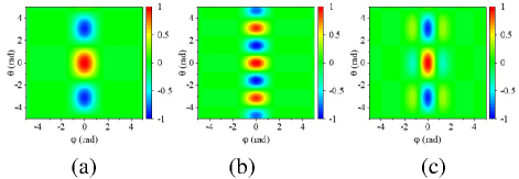
Figure 1: Instances of the fluctuation patterns attributed to the varied angular frequency parameters ${\omega }_1$ and ${\omega }_2$. (a) $l_1=1,l_2=7,{\omega }_1={\omega }_2=1$, (b) $l_1=1,l_2=7,{\omega }_1=1,{\omega }_2=2$, (c) $l_1=1,l_2=7,{\omega }_1=2,{\omega }_2=1$.

To further illustrate the adaptability of the improved POI kernel function to the RCS patterns of complex targets, we analyzed the spectral properties of these two kernel functions.

First, consider the 1D case ($\theta$-direction):

$$K_p^{\prime }(\mathit{\text{x}},{\mathit{\text{x}}}^{\prime })=\cos [\omega (x-x^{\prime })]\exp \left(-\frac{{(x-x^{\prime })}^2}{2l^2}\right).$$

(8)

The Fourier transform of this kernel is derived as follows:

This result shows that the improved POI kernel acts as dual Gaussian bandpass filters centered at ${\omega }^{\prime }=\pm \omega$, with bandwidth controlled by $l$.

For 2D RCS modeling, we have:

$$ℱ\{K_p^{\prime }\}({\omega }_1^{\prime },{\omega }_2^{\prime })\propto \prod _{i=1}^2\left[\begin{array}{c}\exp \left(-\frac{l_i^2{({\omega }_i^{\prime }-{\omega }_i)}^2}{2}\right)\hfill \\ +\exp \left(-\frac{l_i^2{({\omega }_i^{\prime }+{\omega }_i)}^2}{2}\right)\hfill \end{array}\right].$$

(10)

This structure allows the improved POI kernel function to adaptively amplify frequency components near $(\pm {\omega }_1,\pm {\omega }_2)$. However, the POI kernel only amplifies frequency components near $(\pm 1,\pm 1)$.

The improved POI kernel function introduces angular frequency parameters ${\omega }_1$ and ${\omega }_2$, which can automatically adjust the center frequency of the filter according to the actual fluctuation frequency of the target’s RCS (matching the multi-harmonic RCS spectrum). In this way, whether for simple or complex targets, the SVR model can find the most matching frequency to capture the RCS fluctuations. In contrast, the center frequency of the filter corresponding to the POI kernel function is fixed, easily lead to underfitting.

B. Proposed data preprocessing method

In the IEEE dictionary of electrical and electronics terms, the definition of RCS is given by the following expression:

$$\sigma =\underset{r\to \mathrm{\infty }}{lim}4\pi r^2\frac{{\left|{\mathit{\text{E}}}_{\mathrm{scat}}\right|}^2}{{\left|{\mathit{\text{E}}}_{\mathrm{inc}}\right|}^2},$$

(11)

where ${\mathit{\text{E}}}_{\mathrm{inc}}$ is the incident field. The unit of $\sigma$ is ${\mathrm{m}}^2$. Assuming $\left|{\mathit{\text{E}}}_{\mathrm{inc}}\right|=1\mathrm{V}/\mathrm{m}$, then (11) can be simplified to:

$$\sigma =\underset{r\to \mathrm{\infty }}{lim}4\pi r^2{\left|{\mathit{\text{E}}}_{\mathrm{scat}}\right|}^2.$$

(12)

In the academic and industrial communities, it is also customary to use the following notation:

$${\sigma }_{\mathrm{dB}}=10\lg (\sigma ),$$

(13)

where the unit of ${\sigma }_{\mathrm{dB}}$ is dBsm.

It is noteworthy that $K_P^{\prime }(\mathit{\text{x}},{\mathit{\text{x}}}^{\prime })$ is derived from the scattered field formula presented in (2) and, thus, it is more apt for modeling the scattered field rather than modeling the target’s RCS directly. Hence, we propose transforming the target’s RCS into the magnitude of the scattered field $\left|{\mathit{\text{E}}}_{\mathrm{scat}}\right|$. Therefore, according to (12) and (13), we have:

$$\left|{\mathit{\text{E}}}_{\mathrm{scat}}\right|=\sqrt{\frac{\sigma }{4\pi r^2}}=\sqrt{\frac{{10}^{{\sigma }_{\mathrm{dB}}/10}}{4\pi r^2}}.$$

(14)

Then, convert it into normalized scattered field strength:

$${\tilde{E}}_{\mathrm{scat}}=\frac{\left|{\mathit{\text{E}}}_{\mathrm{scat}}\right|-\left|{\mathit{\text{E}}}_{\mathrm{scat}}^{\min }\right|}{\left|{\mathit{\text{E}}}_{\mathrm{scat}}^{\max }\right|-\left|{\mathit{\text{E}}}_{\mathrm{scat}}^{\min }\right|},$$

(15)

where $\left|{\mathit{\text{E}}}_{\mathrm{scat}}^{\max }\right|$ and $\left|{\mathit{\text{E}}}_{\mathrm{scat}}^{\max }\right|$ denote the maximum and the minimum scattered field strengths, respectively.

C. Training of APOI-SVR

This subsection primarily outlines the methodology for constructing APOI-SVR on previous derivations to model the target’s RCS characteristics. The core focus is training APOI-SVR with sampled RCS data. Training APOI-SVR is essentially solving an optimization problem with constrains, that is:

$$\begin{array}{c}\underset{\alpha ,\widehat{\alpha }}{max}\sum _{i=1}^n{y}_i({\alpha }_i-{\widehat{\alpha }}_i)-\epsilon ({\alpha }_i+{\widehat{\alpha }}_i)\hfill \\ -\frac{1}{2}\sum _{i=1}^n\sum _{j=1}^n({\alpha }_i-{\widehat{\alpha }}_i)({\alpha }_j-{\widehat{\alpha }}_j)K_P^{\prime }({\mathit{\text{x}}}_i,{\mathit{\text{x}}}_j)\hfill \\ \mathrm{s}.\mathrm{t}.\sum _{i=1}^n({\alpha }_i-{\widehat{\alpha }}_i)=0,{\alpha }_i,{\widehat{\alpha }}_i\in [0,𝒞]\hfill \end{array},$$

(16)

where $\epsilon$ represents the width of the insensitive tube, and $𝒞$ is the penalty parameter. Assuming that $n$ RCS data of the target, denoted as $\{({\theta }_i,{\phi }_i,{\sigma }_i)|i=1,\mathrm{\dots },n\}$, have been collected, the steps are as follows:

1. Data preprocessing: Apply (14) and (15) to preprocess the RCS data for training APOI-SVR.

2. Hyperparameter optimization: Adopt the Bayesian optimization method [23, 24] to obtain optimal values of hyperparameter l1, l2, ω1, ω2, and C . In this work, an open-source Python library called “BayesO” is adopted.

3. Model establishment: Retrain APOI-SVR with these optimal hyperparameters to establish the approximation model for ˜Escat(θ,ϕ): where αi, αˆ i and b are obtained by solving (16) with the sequential minimal optimization (SMO) [25].

4. RCS modeling: Based on (14), (15) and (17), establish the following surrogate model for modeling the target’s RCS:

The overall flowchart of applying APOI-SVR for efficient modeling of the target’s RCS is illustrated in Fig. 2. The improvements compared with POI-SVR [22] are marked with cyan.

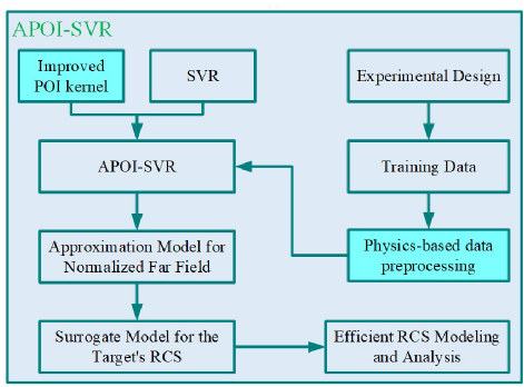
Fig. 2. Flowchart illustrating the application of APOISVR for efficient RCS modeling of a target.

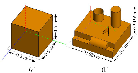
Fig. 3. Two exemplary targets for the validation of the proposed APOI-SVR. (a) Conducting Cube with the side length of 0.5 m and (b) full-sized conducting SLICY model with dimensions of 0.5625 m × 0.5 m × 0.3436 m.

III. VALIDATION RESULTS

A. Accuracy of APOI-SVR

In this section, we evaluate the performance of the proposed APOI-SVR across three critical dimensions: the accuracy of APOI-SVR in predicting the target’s RCS, the efficiency of APOI-SVR in terms of model construction and prediction, and the applicability of APOI-SVR in rapidly modeling and analyzing the RCS of real-world targets.

In this subsection, we assess the modeling accuracy of APOI-SVR utilizing the training datasets CVtrain and SHtrain, which correspond to the simple Cube model and the complex SLICY model, respectively. Equal training and hyperparameter optimization procedures are applied to both datasets, followed by numerical validations on the corresponding test datasets, CVtest and SHtest. The results are shown in Figs. 4 and 5, offering a comparative analysis between the RCS prediction accuracy of POI-SVR and APOI-SVR.

Figure 4 details the test results for the simple Cube model. Figure 4 (a) presents the performance of POI-SVR, with a root mean square error (RMSE) of 1.056926 and a coefficient of determination (R${}^{\mathrm{2}}$) of 0.987702. In contrast, Fig. 4 (b) displays the superior performance of APOI-SVR, with a reduced RMSE of 0.795794 and a higher R${}^{\mathrm{2}}$ of 0.993028. Figure 5 showcases the results for the complex SLICY model. Similar to the Cube model, APOI-SVR exhibits a higher precision in predicting the RCS of the complex SLICY model, as evidenced by a lower RMSE of 0.448094 and a higher R${}^{\mathrm{2}}$ of 0.994632 shown in Fig. 5 (b). As a competitor, POI-SVR obtains RMSE and R${}^{\mathrm{2}}$ of 0.651156 and 0.994097, respectively. Table 2 enumerates the RMSE reduction ratios of APOI-SVR compared with POI-SVR. Specifically, APOI-SVR reduces the predictive RMSE by 24.71% for the Cube model and by 31.18% for the SLICY model.

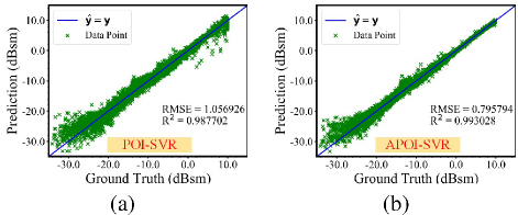
Figure 4: Test results for the simple Cube model: (a) POI-SVR and (b) APOI-SVR.

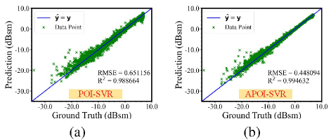
Figure 5: Test results for the complex SLICY model: (a) POI-SVR and (b) APOI-SVR.

Table 2: Predictive RMSE reduction ratios of APOI-SVR compared with POI-SVR

Target	Predictive RMSE	Reduction
	POI-SVR	APOI-SVR
Cube	1.056926	0.795794	24.71%
SLICY	0.651156	0.448094	31.18%

Additionally, the absolute error distributions of POI-SVR and APOI-SVR are analyzed. Figure 6 presents the comparisons between the absolute error distributions of POI-SVR and APOI-SVR across both the Cube model and the SLICY model. In the case of the Cube model, the absolute errors of APOI-SVR are primarily within the range of 0.0 to 2.0 dBsm, whereas POI-SVR displays a broader spread up to 3.0 dBsm. Similarly, in the case of the SLICY model, APOI-SVR maintains a tighter error range of 0.0 to 1.0 dBsm. demonstrating its robustness in handling complex targets.

On the whole, whether for the simple Cube model or the complex SLICY model, APOI-SVR achieves lower RCS prediction errors compared with POI-SVR. This indicates the effectiveness of the improved POI kernel function (see section IIA) and the physics-based data preprocessing method (see section IIB) in enhancing the RCS prediction accuracy of SVR, thereby offering a reliable and accurate modeling tool that facilitates the efficient analysis of the target’s RCScharacteristics.

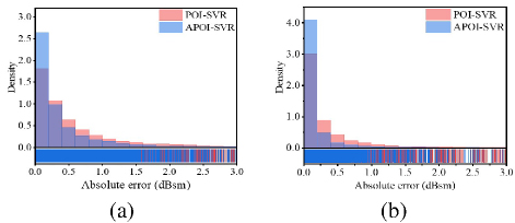
Figure 6: Comparisons of absolute error distributions: (a) Cube and (b) SLICY.

B. Efficiency of APOI-SVR

In practical applications, the efficacy of an ML model is not solely appreciated by its prediction accuracy but also significantly by its implementation efficiency, including the time costs of optimizing hyperparameters with Bayesian optimization method and subsequent model retraining with the determined optimal hyperparameters, as well as the efficiency of the prediction process. Although the introduction of hyperparameters ${\omega }_1$ and ${\omega }_2$ into the improved POI kernel function significantly boosts the representation capability of APOI-SVR, it is essential to investigate any potential trade-offs in efficiency. Hence, a comprehensive analysis of both the implementation and prediction efficiency of APOI-SVR is warranted. It should be noted that, to ensure a compelling comparison, all time costs presented in this paper are obtained under single-core operation with an Intel Core 2 Duo CPU T6670.

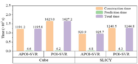
Figure 7: Time cost comparison between POI-SVR and APOI-SVR.

Table 3: Time costs and optimization iterations of hyperparameter optimization in the model implementation stage

Target	APOI-SVR	POI-SVR
	Optimization Time Cost (s)	Optimization Iteration	Time Cost per Iteration (s)	Optimization Time Cost (s)	Optimization Iteration	Time Cost per Iteration (s)
Cube	1171.6	60	19.5	1617.6	100	16.2
SLICY	920.9	50	18.1	1224.7	80	15.3

Figure 7 illustrates the time costs of APOI-SVR and POI-SVR, including implementation, prediction, and total times for both the Cube and SLICY models. It can be seen that in terms of implementation time, APOI-SVR takes less than POI-SVR. This reduction is attributed to the fact that, although the training time per iteration of APOI-SVR is slightly increased, the proposed physics-based data preprocessing method results in fewer optimization iterations necessary to reach convergence to the optimal solution (see Table 3). Consequently, the implementation time for APOI-SVR is shorter than that for POI-SVR. Regarding prediction time, the well-trained APOI-SVR and POI-SVR show negligible differences (less than 1.0 second). Finally, in terms of total time cost, APOI-SVR is less expensive than POI-SVR. Therefore, APOI-SVR surpasses POI-SVR in terms of overall efficiency.

C. Application of APOI-SVR

Having established the superior accuracy and efficiency of APOI-SVR in the previous subsections, we now apply APOI-SVR to analyze the RCS characteristics of a real-world target. Figure 8 depicts the aircraft model under consideration. Given its geometric symmetry, training data are sampled within the region where $\theta$ is in $[0^{\circ },{90}^{\circ }]$ and $\phi$ is in $[0^{\circ },{180}^{\circ }]$. In total, 1296 training samples are collected, preprocessed and subsequently used to train APOI-SVR. The well-trained APOI-SVR is ultimately applied to analyze the aircraft’s RCS characteristics in the upper half space.

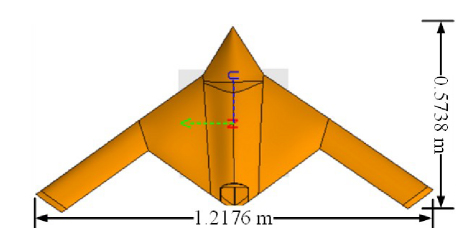
Figure 8: Aircraft model for the illustration of efficient RCS modeling and analysis applying APOI-SVR.

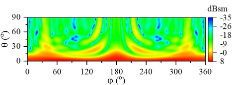
Figure 9: RCS feature map of the aircraft obtained by APOI-SVR.

The frequency of the incident electromagnetic wave is set to 1.0 GHz. Figure 9 depicts the aircraft’s RCS feature map, a 91$\times$361 matrix, obtained by APOI-SVR. For comparison, the results acquired by MLFMA are given in Fig. 10. It can be observed that the results obtained by the two methods are highly consistent, indicating the reliability of APOI-SVR. However, it is worth noting that there is a significant difference in time cost (see Table 4). The total time cost of our APOI-SVR, containing data sampling, hyperparameter optimization, model training, and RCS prediction, is one-twelfth of that demanded by using MLFMA. This demonstrates the practicality of APOI-SVR for efficient RCS modeling of real-world targets.

Table 4: Time costs of acquiring the RCS feature map by APOI-SVR and MLFMA

Method	Sampling/Simulation Time Cost (s)	Optimization Time Cost (s)	Training Time Cost (s)	Prediction Time Cost (s)	Total Time Cost (s)
APOI-SVR	92738.9	1124.8	18.7	1.5	95509.6
MLFMA	1178628.5	—	—	—	1178628.5

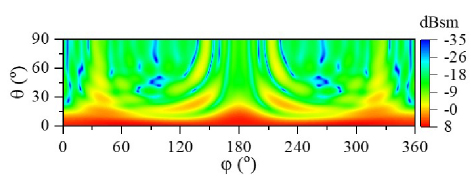
Figure 10: RCS feature map of the aircraft acquired by MLFMA.

IV. CONCLUSION

This paper proposes an advanced physical optics-inspired support vector regression (APOI-SVR) for the efficient modeling of a complex target’s RCS. Two angular frequency parameters are introduced into the physical optics-inspired kernel function to address the various fluctuation patterns of RCS for complex targets, and a physics-based data preprocessing method is proposed to enable the model to efficiently learn the directly related physical quantity, i.e., the normalized electric field. Numerical validations conducted on both a simple Cube model and a complex SLICY model have confirmed that, compared with POI-SVR, the new-proposed APOI-SVR effectively reduces the RMSE in RCS prediction by over 24.7%. Moreover, it maintains high predictive efficiency, capable of completing the prediction of 10,000 samples in the test dataset within 5.0 seconds. Notably, although the introduction of two angular frequency parameters slightly increases the training time for each iteration in the hyperparameter optimization process, the proposed physics-based data preprocessing method reduces the required number of optimization iterations. As a result, in terms of overall efficiency, APOI-SVR outperforms POI-SVR.

Additionally, the application of APOI-SVR to an aircraft model has illustrated its practical efficacy in generating RCS feature maps with high precision and efficiency compared to the well-known MLFMA. This practical application indicates that APOI-SVR may be a valuable tool in the field of electromagnetic scattering analysis. Future research will commit to expanding the applicability of APOI-SVR, including the enhancements tailored for complex targets with coatings.

ACKNOWLEDGMENT

This work is based on the research supported in part by the Postdoctoral Fellowship Program (Grade C) of China Postdoctoral Science Foundation under Grant Number GZC20241307, and in part by the National Natural Science Foundation of China under Grant 62231021, Grant 62071347, and Grant 62171335.Corresponding author: Donghai Xiao.

REFERENCES

[1] M. I. Skolnik, Radar Handbook, 3rd ed. New York, NY: McGraw-Hill, 2008.

[2] E. F. Knott, J. F. Schaeffer, and M. T. Tulley, Radar Cross Section, 2nd ed. Rayleigh, NC: SciTech, 2004.

[3] M. Cavagnaro, E. Pittella, and S. Pisa, “Numerical evaluation of the radar cross section of human breathing models,” Applied Computational Electromagnetics Society (ACES) Journal, vol. 30, no. 12, pp. 1354-1359, Aug. 2015.

[4] R. Haupt, S. Haupt, and D. Aten, “Evaluating the radar cross section of maritime radar reflectors using computational electromagnetics,” Applied Computational Electromagnetics Society (ACES) Journal, vol. 24, no. 4, pp. 403-406, Aug. 2009.

[5] M. M. Sheikh, “Analysis of reader orientation on detection performance of Hilbert curve-based fractal chipless RFID tags,” Applied Computational Electromagnetics Society (ACES) Journal, vol. 39, no. 6, pp. 490-504, June 2024.

[6] J.-M. Jin, The Finite Element Method in Electromagnetics. Hoboken, NJ: Wiley-IEEE Press, 2014.

[7] C. Qin, X. Wang, and N. Zhao, “EMFEM: A parallel 3D modeling code for frequency-domain electromagnetic method using goal-oriented adaptive finite element method,” Comput. Geosci., vol. 178, Art. no. 105403, Sep. 2023.

[8] F. L. Teixeira, C. Sarris, Y. Zhang, D.-Y. Na, J.-P. Berenger, Y. Su, M. Okoniewski, W. C. Chew, V. Backman, and J. J. Simpson, “Finite-difference time-domain methods,” Nature Rev. Methods Primers, vol. 3, p. 75, 2023.

[9] A. Taflove and S. C. Hagness, Computational Electromagnetics: The Finite-Difference Time-Domain Method, 2nd ed. Norwood, MA: Artech House, 2000.

[10] P. D. Cannon and F. Honary, “A GPU-accelerated finite-difference time-domain scheme for electromagnetic wave interaction with plasma,” IEEE Trans. Antennas Propagat., vol. 63, no. 7, pp. 3042-3054, July 2015.

[11] T. Maceina, P. Bettini, G. Manduchi, and M. Passarotto, “Fast and efficient algorithms for computational electromagnetics on GPU architecture,” IEEE Trans. Nucl. Sci., vol. 64, no. 7, pp. 1983-1987, July 2017.

[12] Y. Xu, H. Ma, and R. Jiang, “Collaborating CPU and GPU for the electromagnetic simulations with the FDTD algorithm,” Concurrency Comput., Pract. Exper., vol. 29, no. 4, p. e3859, Feb.2017.

[13] W.-W. Zhang, D.-H. Kong, X.-Y. He, and M.-Y. Xia, “A machine learning method for 2-D scattered far-field prediction based on wave coefficients,” IEEE Antennas Wireless Propag. Lett., vol. 22, no. 5, pp. 1174-1178, May 2023.

[14] R. Weng, D. Sun, W. Yang, X. Chen, and W. Lu, “Efficient broadband monostatic RCS computation of morphing S-Shape cavity using artificial neural networks,” IEEE Antennas Wireless Propag. Lett., vol. 22, no. 2, pp. 263-267, Feb. 2022.

[15] J. Wu, C. Liu, L. Yang, and L. Tang, “Research on RCS sequence prediction based on ARIMA-TPA-LSTM algorithm,” in 2023 China Automation Congress (CAC), Chongqing, China, pp. 1887-1892, Nov. 2023.

[16] H. Drucker, C. J. Burges, L. Kaufman, A. Smola, and V. Vapnik, “Support vector regression machines,” in Proc. Int. Conf. Neural Inf. Process. Syst., pp. 155-161, 1997.

[17] D. Basak, S. Pal, and D. C. Patranabis, “Support vector regression,” in Proc. Neural Inf. Process. Lett. Rev., vol. 11, no. 10, pp. 203-224, 2007.

[18] M. Awad and R. Khanna, “Support vector regression,” in Efficient Learning Machines, Mariette Awad and Rahul Khanna, Eds. Berlin, Germany: Springer, 2015, pp. 67-80.

[19] Z. Zhang, P. Wang, and M. He, “Wideband monostatic RCS prediction of complex objects using support vector regression and grey-wolf optimizer,” Applied Computational Electromagnetics Society (ACES) Journal, vol. 38, no.8, pp. 609-615, Aug. 2023.

[20] Z. Zhang and M. He, “Fast prediction of electromagnetic scattering fields based on machine learning and PSO algorithm,” in 2022 IEEE 10th Asia-Pacific Conference on Antennas and Propagation (APCAP), Xiamen, China, pp. 1-2, 2022.

[21] C. Dong, X. Meng, L. Guo, and J. Hu, “3D sea surface electromagnetic scattering prediction model based on IPSO-SVR,” Remote Sens., vol. 14, no. 18, p. 4657, Sep. 2022.

[22] D. Xiao, L. Guo, W. Liu, and M. Hou, “Efficient RCS prediction of the conducting target based on physics-inspired machine learning and experimental design,” IEEE Trans. Antennas Propag., vol. 69, no. 4, pp. 2274-2289, Apr. 2021.

[23] J. Snoek, H. Larochelle, and R. P. Adams, “Practical Bayesian optimization of machine learning algorithms,” in Proc. Adv. Neural Inf. Process. Syst., pp. 2951-2959, 2012.

[24] J. Kim and S. Choi, “BayesO: A Bayesian optimization framework in Python,” J. Open Source Softw., vol. 8, no. 90, p. 5320, Oct. 2023.

[25] G. W. Flake and S. Lawrence, “Efficient SVM regression training with SMO,” Mach. Learn., vol. 46, nos. 1-3, pp. 271-290, 2002.

BIOGRAPHIES

Chenge Shi received her M.S. and Ph.D. degrees in Radio Physics from Xidian University, Xi’an, Shaanxi, China, in 2017 and 2023, respectively. She is currently a Researcher with AVIC Xi’an Aircraft Industry Group Company Ltd., primarily interested in aircraft manufacturing and testing.

Rui Cai received his B.S. degree from Xidian University in 2011, and has been enthusiastically contributing to AVIC Xi’an Aircraft Industry Group Company Ltd. He is a Senior Engineer, mainly engaged in the demonstration of test scheme and system simulation.

Wei Dong is the Chief Engineer of AVIC Xi’an Aircraft Industry Group Company Ltd. He is mainly engaged in the testing of modern airborne systems, which include electromechanical components, avionics, and flight control systems.

Donghai Xiao received the B.S. degree in Applied Physics and the Ph.D. degree in Radio Physics from Xidian University, Xi’an, China, in 2014 and 2023, respectively. He is currently a Postdoctoral Researcher with Hangzhou Institute of Technology, Xidian University, Hangzhou, China. His research interests include the areas of computational electromagnetics, radar signal processing and machine learning.

ACES JOURNAL, Vol. 40, No. 4, 309–316
doi: 10.13052/2024.ACES.J.400404
© 2025 River Publishers