Fast Direct LDL${}^{\mathrm{\prime }}$ Solver for Method of Moments Electric Field Integral Equation Solution

Yoginder Kumar Negi${}^{\mathbf{\text{1}}}$, N. Balakrishnan${}^{\mathbf{\text{1}}}$, and Sadasiva M. Rao${}^{\mathbf{\text{2}}}$

¹Supercomputer Education and Research Center
Indian Institute of Science, Bangalore 560012, India
yknegi@gmail.com, balki@iisc.ac.in

²Naval Research Laboratory
Washington DC 20375, USA
sadasiva.rao@nrl.navy.mil

Submitted On: December 16, 2024; Accepted On: March 26, 2025

ABSTRACT

This paper proposes a new fast direct solver using the block diagonalization method. In our proposed method, the symmetric half single-level compressed block matrix is factorized using the diagonalization method into block diagonal and upper triangle block ${\mathit{\text{LDL}}}^{\prime }$ format where, due to symmetric property, L is a transpose of ${\mathit{\text{L}}}^{\prime }$. The far-field blocks in the upper triangle row block are merged and compressed using Adaptive Cross Approximation (ACA) and QR factorization. The solution consists of solving the diagonal block matrix and matrix-vector multiplication of the compressed row blocks of the upper triangle matrices. Our results show that the factorization cost and memory scales to $O(N^{1.5})$ and the solution process scales to $O(N)$. The method generates an efficient solution process for solving large-scale electromagnetics problems.

Index Terms: Adaptive Cross Approximation (ACA), Electric Field Integral Equation (EFIE), electromagnetics scattering, fast direct solver, matrix compression, Method of Moments (MoM).

I. INTRODUCTION

Method of Moments (MoM) is a well-known integral equation-based Computational Electromagnetics (CEM) [1] method for solving complex electromagnetic radiation and scattering problems numerically in the frequency domain. Compared to differential equation-based methods like Finite Element Method (FEM) [2] and Finite Difference Time Domain (FDTD) [3] methods, MoM is free from grid dispersion error and leads to a smaller matrix size than FEM. The MoM application for solving large-scale electromagnetics problems is limited by dense matrix computation property with the matrix computation and storage cost of $O(N^2)$ for N number of unknowns. Solving the MoM dense matrix with a direct solver leads to $O(N^3)$ computation cost and with iterative solver leads to $N_{itr}O(N^2)$ cost for $N_{itr}$ iteration count with $O(N^2)$ matrix-vector product cost. The high matrix computation, storage, and solution cost is mitigated by various matrix compression-based fast solver algorithms proposed by various researchers. The matrix compression for fast solvers may be of two categories: analytical-based compression and algebraic matrix compression. Examples of analytic-based compression methods are Multilevel Fast Multipole Algorithm (MLFMA) [4], Adaptive Integral Method (AIM) [5], and pre-corrected FFT [6]. Similarly, we have algebraic matrix compressed methods like Adaptive Cross Approximation (ACA) [7, 8], IE-QR [9], and H-Matrix [10, 11, 12]. Analytical fast solvers are kernel-dependent, whereas algebraic fast solvers are kernel-independent and easy to implement. All the fast solvers work on reducing matrix filling, solution, and storage time. Full wave fast solver in CEM reduces matrix filling and storage time to $O(NlogN$). However, the matrix solution time depends on the method of solution and whether the algorithm adopts an iterative approach or a direct approach. For the iterative solution, the solution time scales as $N_{itr}O(NlogN$) for $O(NlogN)$ compressed matrix-vector product cost. The solution of these methods relies on the compressed matrix’s iterative solution. The iterative solution process is a convergence-dependent method for each matrix-vector product iteration. Furthermore, the convergence for each iteration depends on the condition number of the matrix computed. It is well-known that the Electric Field Integral Equation (EFIE) [13] gives an ill-conditioned MoM matrix. This ill-conditioning due to the closed geometry structure can be overcome by using a Magnetic Field Integral Equation (MFIE) [14] and a Combined Field Integral Equation (CFIE) [15]. Also, the ill-conditioning may be due to structural geometry or mesh quality. The ill-conditioning leads to a high iteration count when solved with an iterative solver. The high iteration is mitigated by using various matrix preconditioners [16, 17, 18]. The preconditioner computation comes with the extra precondition computation cost and precondition solution cost during the iterative solution process.

Solving multiple right-hand side (RHS) electromagnetics problems like in monostatic radar cross section (RCS) computation or multiport microwave network system analysis with a fast iterative solver may lead to high solution time. The overall solution time will scale to $N_{rhs}{N}_{itr}O(NlogN)$ for $N_{rhs}$ RHS. Also, for a multi-RHS or single-RHS system, the number of unknowns increases with the increase in simulation frequency or geometry size. With the increase in the number of unknowns, solving the linear system of equations with an iterative, fast solver will lead to a further increase in the number of iterations ($N_{itr}$) for the solution process.

The lacuna of the iterative solver for solving linear systems of equations is overcome by using direct matrix solution methods. Direct solvers are the most reliable method for solving any linear system of equations, with a guaranteed solution for the system. However, the high factorization and solution costs hinder the application of direct solvers for significant electromagnetic problems. In the past decade, there has been an inclination among the fast solver research community to develop direct solution-based fast solvers. MLFMA-based analytical fast direct solvers proposed in [19, 20] are kernel-dependent. Algebraic fast direct solvers built upon extended matrix [21] and $H^2$-Matrix [22] does not scale well for significant problems. A power series-based fast direct solver is proposed in [23, 24], where the solution convergence depends on the matrix’s condition number. Sherman-Morrison-Woodbury based fast direct solvers [25, 26] have high factorization and solution time. A LU-based fast direct solver is proposed in [27, 28, 29], and factorization is applied to a single-level compressed MoM matrix. LU matrix factorization and solutions are serial and difficult to parallelize.

This work proposes a new fast direct solver based on the diagonalization applied on a symmetric half single-level compressed block MoM matrix. The factorization cost is reduced by applying low-rank block matrix operation, and the linear cost of the matrix solution is achieved by merging the compressed far-field matrix blocks into a single compressed matrix block. The solution process consists of block diagonal matrix solution and matrix-vector product of the row block compress matrices. The paper is organized as follows: section II presents a brief description of EFIE MoM with block matrix compression. In section III, we present the proposed block diagonalized fast direct solver. Section III also presents the low-rank matrix operation performed on the compressed matrices to reduce the factorization and solution time. In section IV, the efficiency and accuracy of the proposed fast direct solver is presented. Section V concludes the paper.

II. BRIEF DESCRIPTION OF EFIE-MOM

The MoM matrix is computed for 3D surfaces using EFIE, MFIE, or CFIE formulations. Selection of the integral equation method is essential when solving the matrix with a regular iterative solver. MFIE is only applicable for closed-body geometries. CFIE is a combination of EFIE and MFIE, which further increases matrix computation time. For the sake of clarity, this work uses only EFIE for MoM matrix computation to solve 3D Perfect Electric Conductor (PEC) geometry and can be easily extended to MFIE and CFIE. The governing equation for EFIE is:

$$E_{total}=E_{inc}+E_{scatt},$$

(1)

where $E_{total}$ is the total electric field equal to the sum of the incident electric field ($E_{inc}$ ) and the scattered electric field ($E_{scatt}$). Applying the boundary condition, expanding current density ($J(r^{\prime })$) and charge density ($\rho (r^{\prime })$) for the electric field vector potential and scalar potential with the RWG [30] basis functions ($f_i$), and performing Galerkin testing, the elements of the MOM matrix are:

	$\mathit{\text{Z}}(i,j)$	$={\displaystyle \frac{j\omega \mu }{4\pi }}{\displaystyle \iint f_i\cdot f_j\frac{e^{-jk\left|r-r^{\prime }\right|}}{r-r^{\prime }}\mathit{d}s\mathit{d}t}+{\displaystyle \frac{1}{j\omega 4\pi \epsilon }}{\displaystyle \iint \nabla }$
		$\mathrm{\hspace{1em}\hspace{1em}}{f}_i{\displaystyle \frac{e^{-jk\left|r-r^{\prime }\right|}}{r-r^{\prime }}}\nabla \cdot f_{j}dsdt.$		(2)

In the above equation, the MoM matrix element is computed for the $i^{th}$ test $j^{th}$ source basis. In equation (II.), $k$ is the wavenumber, $r$ and $r^{\prime }$ represent the observer and source points, and $\mu$ and $\epsilon$ are the permeability and permittivity of the background material. Integration is performed over the RWG source and testing domains. MoM matrix computation using equation (II.) leads to a linear system of equations. The system of equations can be written as a combination of a near-field interaction matrix ${\mathit{\text{Z}}}_{\mathit{\text{N}}}$and a far-field interaction matrix ${\mathit{\text{Z}}}_{\mathit{\text{F}}}$ given by:

$$\left[{\mathit{\text{Z}}}_{\mathit{\text{N}}}+{\mathit{\text{Z}}}_{\mathit{\text{F}}}\right]\mathit{\text{x}}=\mathit{\text{b}}.$$

(3)

Solving equation (3) for x presents computation time and memory limitations, which can be overcome by applying various fast solver methods. These methods work on the compressibility of the far-field matrix.

For the computation of a fast solver, the mesh of the 3D geometry is divided into small blocks using the multilevel binary-tree or oct-tree partition method [12]. The fast solver is the single level when the far-field matrix compression is carried out at the lowest level, and the multilevel is when the matrix compression is done at all levels. Single-level fast solver reduces matrix filling and solution time to $O(N^{1.5})$ whereas multilevel reduces the time complexity to $O(NlogN)$. This work uses a single-level compressed MoM block matrix fast solver to ease block matrix operation. For the single-level fast solver matrix construction, matrix compression is applied at the lowest level of binary-tree-based 3D geometry decomposition, and the interaction is computed for the mesh block satisfying the admissibility condition [12]. At the leaf level, the block interaction that does not satisfy the admissibility condition is considered a near-field interaction. Further, this work employs the re-compressed ACA method [31] to compute a symmetric single-level compressed block matrix. The compressed matrix is made symmetric by averaging the upper diagonal and lower diagonal values and replacing the upper diagonal and lower diagonal values with the average value. Using the symmetric property, we can reuse the upper diagonal value for matrix-vector product and matrix factorization. Exploiting the symmetric property, we compute and save the diagonal and upper diagonal matrix in the compressed far-field and dense near-field blocks [12]. The single-level symmetric half-compressed block matrix is used for factorization and solution process. The formulation for the new fast direct solver with reduced factorization and solution time is discussed in the next section.

III. FAST DIRECT SOLVER

This section discusses the factorization and solution process for developing a fast direct solver applied on a single-level compressed block matrix. The matrix diagonalization process has previously been used to solve the linear system of equations for sparse and dense matrices [32, 33, 34]. However, these methods lead to a high cost of factorization and solution. In our previous work [18, 23, 24], the diagonalization of the near-field block matrix is discussed in detail. There, the computation is performed on the dense near-field block matrices. Due to the dense nature of the near-field matrix, the cost of computation and storage is kept low. Extending the diagonalization method to a fast solver-based full matrix is limited by the far-field matrix blocks. In this work, we diagonalize the full MoM compressed matrix. To understand the complete implementation of the factorization process, we will discuss the factorization process for the whole matrix in detail. The far-field matrix operation cost is reduced by performing low-rank block matrix operation. The method is applied to the MoM matrix to factorize it to ${\mathit{\text{LDL}}}^{\prime }$ format, where D is a diagonal block matrix and L and ${\mathit{\text{L}}}^{\prime }$ are lower and upper triangle block matrices. The lower triangle block matrix L is the transpose of the upper triangle block matrix, leading to computation and memory savings. In the following subsection, details of the diagonalization process, along with the ways to make it faster for set-up and solution matrix-vector product, are presented.

A. Block matrix factorization

Gaussian Elimination is a well-known method for diagonalizing dense or sparse block matrices. The Gaussian Elimination is performed over the single-level symmetric compressed block matrix. An asymmetric compressed block matrix is computed for the mesh geometry divided into mesh element clusters based on the multilevel binary-tree division. The single-level compressed block matrix near-field and far-field matrix interaction is computed for binary-tree mesh blocks at the lowest level. The symmetric half-block matrix $[\mathit{\text{Z}}]$ for factorization is shown below:

$$[\mathit{\text{Z}}]=\left[\begin{array}{ccc}\hfill {\mathit{\text{Z}}}_{11}\hfill & \hfill {\mathit{\text{Z}}}_{12}\hfill & \hfill \begin{array}{cc}\hfill {\mathit{\text{Z}}}_{13}\hfill & \hfill {\mathit{\text{Z}}}_{14}\hfill \end{array}\hfill \\ \hfill 0\hfill & \hfill {\mathit{\text{Z}}}_{22}\hfill & \hfill \begin{array}{cc}\hfill {\mathit{\text{Z}}}_{23}\hfill & \hfill {\mathit{\text{Z}}}_{24}\hfill \end{array}\hfill \\ \hfill \begin{array}{c}\hfill 0\hfill \\ \hfill 0\hfill \end{array}\hfill & \hfill \begin{array}{c}\hfill 0\hfill \\ \hfill 0\hfill \end{array}\hfill & \hfill \begin{array}{cc}\hfill \begin{array}{c}\hfill {\mathit{\text{Z}}}_{33}\hfill \\ \hfill 0\hfill \end{array}\hfill & \hfill \begin{array}{c}\hfill {\mathit{\text{Z}}}_{34}\hfill \\ \hfill {\mathit{\text{Z}}}_{44}\hfill \end{array}\hfill \end{array}\hfill \end{array}\right].$$

(4)

The above block matrix consists of near- and far-field matrix blocks. The factorization process consists of diagonalizing the above matrix by multiplying it with the right sparse block matrix. The right scaling matrix nullifies the row blocks of the matrix, leaving a diagonal block matrix. Right scaling matrix $[{\mathit{\alpha }}_{\mathbf{1}}]$ for first row blocks is given as:

$$[{\mathit{\alpha }}_1]=\left[\begin{array}{cc}\hfill \begin{array}{cc}\hfill \begin{array}{c}\hfill \begin{array}{c}\hfill {\mathit{\text{I}}}_{11}\hfill \\ \hfill 0\hfill \end{array}\hfill \\ \hfill \begin{array}{c}\hfill 0\hfill \\ \hfill 0\hfill \end{array}\hfill \end{array}\hfill & \hfill \begin{array}{c}\hfill \begin{array}{c}\hfill -{\mathit{\text{Z}}}_{11}^{-1}{\mathit{\text{Z}}}_{12}\hfill \\ \hfill {\mathit{\text{I}}}_{22}\hfill \end{array}\hfill \\ \hfill \begin{array}{c}\hfill 0\hfill \\ \hfill 0\hfill \end{array}\hfill \end{array}\hfill \end{array}\hfill & \hfill \begin{array}{cc}\hfill \begin{array}{c}\hfill \begin{array}{c}\hfill -{\mathit{\text{Z}}}_{11}^{-1}{\mathit{\text{Z}}}_{13}\hfill \\ \hfill 0\hfill \end{array}\hfill \\ \hfill \begin{array}{c}\hfill {\mathit{\text{I}}}_{33}\hfill \\ \hfill 0\hfill \end{array}\hfill \end{array}\hfill & \hfill \begin{array}{c}\hfill \begin{array}{c}\hfill -{\mathit{\text{Z}}}_{11}^{-1}{\mathit{\text{Z}}}_{14}\hfill \\ \hfill 0\hfill \end{array}\hfill \\ \hfill \begin{array}{c}\hfill 0\hfill \\ \hfill {\mathit{\text{I}}}_{44}\hfill \end{array}\hfill \end{array}\hfill \end{array}\hfill \end{array}\right],$$

(5)

where $\begin{array}{cc}\hfill \begin{array}{cc}\hfill {\mathit{\text{I}}}_{11},\hfill & \hfill {\mathit{\text{I}}}_{22}\hfill \end{array},\hfill & \hfill {\mathit{\text{I}}}_{33}\hfill \end{array}$, and ${\mathit{\text{I}}}_{44}$are the identity block matrices. Equations (4) and (5) are combined to scale the first-row blocks of $[\mathit{\text{Z}}]$to diagonal blocks, and the system of the equation is given as:

	$[{\widetilde{\mathit{\text{Z}}}}^1]$	$=\left[\begin{array}{cc}\hfill \begin{array}{cc}\hfill \begin{array}{c}\hfill \begin{array}{c}\hfill {\mathit{\text{Z}}}_{11}\hfill \\ \hfill 0\hfill \end{array}\hfill \\ \hfill \begin{array}{c}\hfill 0\hfill \\ \hfill 0\hfill \end{array}\hfill \end{array}\hfill & \hfill \begin{array}{c}\hfill \begin{array}{c}\hfill {\mathit{\text{Z}}}_{12}\hfill \\ \hfill {\mathit{\text{Z}}}_{22}\hfill \end{array}\hfill \\ \hfill \begin{array}{c}\hfill 0\hfill \\ \hfill 0\hfill \end{array}\hfill \end{array}\hfill \end{array}\hfill & \hfill \begin{array}{cc}\hfill \begin{array}{c}\hfill \begin{array}{c}\hfill {\mathit{\text{Z}}}_{13}\hfill \\ \hfill {\mathit{\text{Z}}}_{23}\hfill \end{array}\hfill \\ \hfill \begin{array}{c}\hfill {\mathit{\text{Z}}}_{33}\hfill \\ \hfill 0\hfill \end{array}\hfill \end{array}\hfill & \hfill \begin{array}{c}\hfill \begin{array}{c}\hfill {\mathit{\text{Z}}}_{14}\hfill \\ \hfill {\mathit{\text{Z}}}_{24}\hfill \end{array}\hfill \\ \hfill \begin{array}{c}\hfill {\mathit{\text{Z}}}_{34}\hfill \\ \hfill {\mathit{\text{Z}}}_{44}\hfill \end{array}\hfill \end{array}\hfill \end{array}\hfill \end{array}\right]$
		$\times \left[\begin{array}{cc}\hfill \begin{array}{cc}\hfill \begin{array}{c}\hfill \begin{array}{c}\hfill {\mathit{\text{I}}}_{11}\hfill \\ \hfill 0\hfill \end{array}\hfill \\ \hfill \begin{array}{c}\hfill 0\hfill \\ \hfill 0\hfill \end{array}\hfill \end{array}\hfill & \hfill \begin{array}{c}\hfill \begin{array}{c}\hfill -{\mathit{\text{Z}}}_{11}^{-1}{\mathit{\text{Z}}}_{12}\hfill \\ \hfill {\mathit{\text{I}}}_{22}\hfill \end{array}\hfill \\ \hfill \begin{array}{c}\hfill 0\hfill \\ \hfill 0\hfill \end{array}\hfill \end{array}\hfill \end{array}\hfill & \hfill \begin{array}{cc}\hfill \begin{array}{c}\hfill \begin{array}{c}\hfill -{\mathit{\text{Z}}}_{11}^{-1}{\mathit{\text{Z}}}_{13}\hfill \\ \hfill 0\hfill \end{array}\hfill \\ \hfill \begin{array}{c}\hfill {\mathit{\text{I}}}_{33}\hfill \\ \hfill 0\hfill \end{array}\hfill \end{array}\hfill & \hfill \begin{array}{c}\hfill \begin{array}{c}\hfill -{\mathit{\text{Z}}}_{11}^{-1}{\mathit{\text{Z}}}_{14}\hfill \\ \hfill 0\hfill \end{array}\hfill \\ \hfill \begin{array}{c}\hfill 0\hfill \\ \hfill {\mathit{\text{I}}}_{44}\hfill \end{array}\hfill \end{array}\hfill \end{array}\hfill \end{array}\right].$		(6)

Equation (6) is represented as:

$$[{\widetilde{\mathit{\text{Z}}}}^1]=\left[\mathit{\text{Z}}\right][{\mathit{\alpha }}_1].$$

(7)

Performing the block matrix and scaling matrix multiplication in the above equation, the first-row block diagonalized matrix block equation is written as:

Equation (A.) gives the diagonalization of the first-row blocks. In the above equation, using the symmetry property, the matrix blocks ${\mathit{\text{Z}}}_{21}$, ${\mathit{\text{Z}}}_{31}$, and ${\mathit{\text{Z}}}_{41}$ are obtained by computing the transpose of${\mathit{\text{Z}}}_{12}$, ${\mathit{\text{Z}}}_{13}$, and ${\mathit{\text{Z}}}_{14}$. So ${\mathit{\text{Z}}}_{21}=\mathit{\text{Z}}^{\prime }{}_{12}$, ${\mathit{\text{Z}}}_{31}=\mathit{\text{Z}}^{\prime }{}_{13}$, and ${\mathit{\text{Z}}}_{41}=\mathit{\text{Z}}^{\prime }{}_{14}$. Likewise, each row block is diagonalized by computing the row scaling matrix block and multiplying it with the row diagonalized matrix. The final diagonalization process is given as:

$$[{\mathit{\text{Z}}}_{\mathit{\text{D}}}]=[{\mathit{\alpha }}_3^{\mathrm{T}}][{\mathit{\alpha }}_2^{\mathrm{T}}][{\mathit{\alpha }}_1^{\mathrm{T}}][\mathit{\text{Z}}][{\mathit{\alpha }}_1][{\mathit{\alpha }}_2]][{\mathit{\alpha }}_3].$$

(9)

Equation (9) written in diagonal form is:

$$[{\mathit{\text{Z}}}_{\mathit{\text{D}}}]=\left[\begin{array}{cc}\hfill \begin{array}{cc}\hfill \begin{array}{c}\hfill \begin{array}{c}\hfill {\mathit{\text{Z}}}_{11}\hfill \\ \hfill 0\hfill \end{array}\hfill \\ \hfill \begin{array}{c}\hfill 0\hfill \\ \hfill 0\hfill \end{array}\hfill \end{array}\hfill & \hfill \begin{array}{c}\hfill \begin{array}{c}\hfill 0\hfill \\ \hfill {\widetilde{\mathit{\text{Z}}}}_{22}\hfill \end{array}\hfill \\ \hfill \begin{array}{c}\hfill 0\hfill \\ \hfill 0\hfill \end{array}\hfill \end{array}\hfill \end{array}\hfill & \hfill \begin{array}{cc}\hfill \begin{array}{c}\hfill \begin{array}{c}\hfill 0\hfill \\ \hfill 0\hfill \end{array}\hfill \\ \hfill \begin{array}{c}\hfill {\widetilde{\mathit{\text{Z}}}}_{33}\hfill \\ \hfill 0\hfill \end{array}\hfill \end{array}\hfill & \hfill \begin{array}{c}\hfill \begin{array}{c}\hfill 0\hfill \\ \hfill 0\hfill \end{array}\hfill \\ \hfill \begin{array}{c}\hfill 0\hfill \\ \hfill {\widetilde{\mathit{\text{Z}}}}_{44}\hfill \end{array}\hfill \end{array}\hfill \end{array}\hfill \end{array}\right].$$

(10)

In equation (10), $[{\mathit{\text{Z}}}_{\mathit{\text{D}}}]$ is the diagonal block matrix D and $[{\mathit{\alpha }}_1][{\mathit{\alpha }}_2]][{\mathit{\alpha }}_3]$ is the upper triangle block matrix U of the LDU factorization. L is the transpose of U due to the symmetric property of the matrix. The block diagonalized system of the equation is written as:

$$[{\mathit{\text{Z}}}_{\mathit{\text{D}}}\mathbf{]}\left[\widetilde{\mathit{\text{x}}}\right]=\left[\widetilde{\mathit{\text{b}}}\right].$$

(11)

Here, $[\mathit{\text{b}}]$ and $[\mathit{\text{x}}]$is computed by:

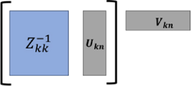
Fig. 1. Low-rank block matrix solution. The matrix operation inside the brackets is performed first to reduce the computation cost.

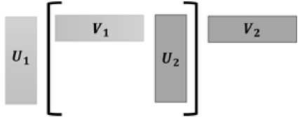
Fig. 2. Low-rank block matrix multiplication operation. Multiplication inside the brackets is performed first for cost saving.

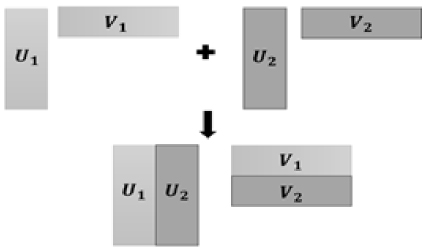
Fig. 3. Low-rank block matrix row and column merging are used to perform low-rank block matrix addition operations.

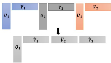
Fig. 4. Conversion of multiple compressed far-field blocks to a single compressed block to reduce matrixvector product cost.

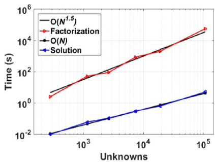
Fig. 5. Block matrix factorization and upper triangle block time using an increasing number of unknowns.

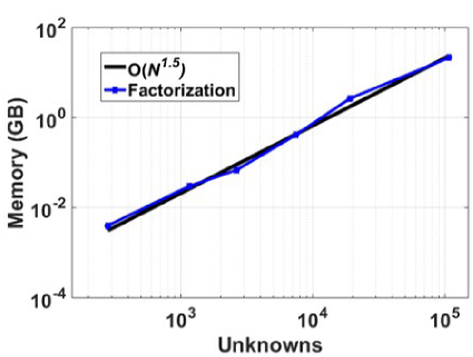
Fig. 6. Factorization memory with an increasing number of unknowns.

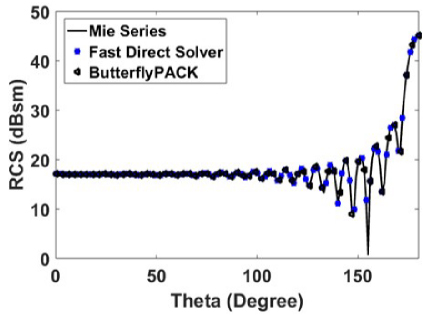
Fig. 7. Bistatic RCS for observation angle θ = 0◦ to 180◦ and φ = 0◦ with incident angle θ = 0◦ and φ = 0◦.

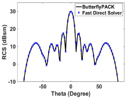
Fig. 8. Monostatic RCS of a square plate for a plane wave incident and observation angle varying from θ = −90◦ to 90◦ and φ = 270◦.

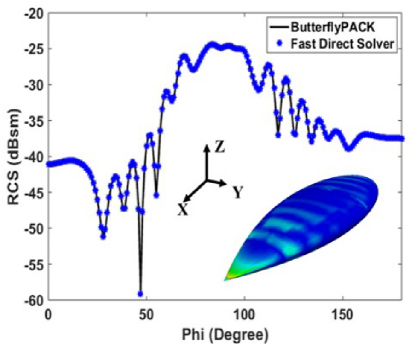
Fig. 9. Monostatic RCS of NASA almond for a plane wave incident and observation angle varying from φ = 0◦ to 180◦ and θ◦ = 90◦.

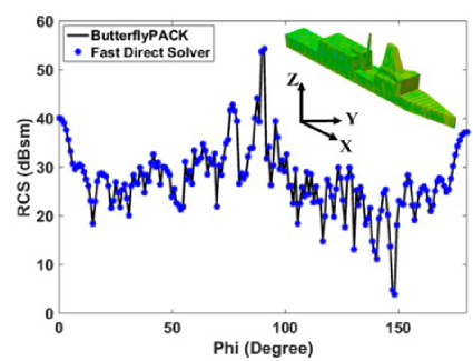
Fig. 10. Monostatic RCS of a ship-like object for a plane wave incident and observation angle varying from φ = 0◦ to 180◦ and θ◦ = 90◦.

VI. CONCLUSION

The work proposed in this paper is a new fast direct solver based on the diagonalization method with the guaranteed solution for the MoM linear system of equa- tions. The single-level symmetric half-compressed block matrix is factorized into LDL′ where D is a diagonal block matrix, and L′ is an upper triangle compressed block matrix. The high cost of diagonalization is over- come using a low-rank block matrix operation process. Our results show the factorization cost scaled to O(N1.5). The solution depends on the block diagonal matrix solu- tion process and matrix-vector product of the upper tri- angle D. The far-field compressed matrices in the upper triangle blocks for each row block are merged further to save matrix-vector product cost and storage memory. Also, the solution process time for the proposed factor- ization scales to O(N). In the current work, the matrix is compressed for the error tolerance of 1e-3. The factor- ization and solution cost can be reduced by compressing the matrix for lower error tolerance 1e-2. The low cost of the solution process, as demonstrated by illustrative examples, makes it highly desirable for solving multi- RHS problems like monostatic RCS computation or mul- tiport network analysis. Unlike block LU factorization and solution process, which is highly serial in nature, in the proposed method, the block operation can be done independently, making the process amendable for effi- cient parallelization for both factorization and solution.

REFERENCES

[1] R. F. Harrington, Field Computation by Moment Methods. Malabar, Florida: Krieger Publishing Co., 1982.

[2] J.-M. Jin, The Finite Element Method in Electromagnetics. Hoboken, New Jersey: John Wiley & Sons, 2015.

[3] A. Taflove and S. C. Hagness, Computational Electrodynamics: The Finite-Difference Time-Domain Method. Norwood, MA: Artech House, 1995.

[4] W. C. Chew, J.-M. Jin, E. Michielssen, and J. Song, Fast and Efficient Algorithms in Computational Electromagnetics. Norwood, MA: Artech House, 2000.

[5] E. Bleszynski, M. Bleszynski, and T. Jaroszewicz, “AIM: Adaptive integral method for solving largescale electromagnetic scattering and radiation problems,” Radio Science, vol. 31, no. 5, pp. 1225-1251, Dec. 1996.

[6] J. R. Phillips and J. K. White, “A pre-corrected FFT method for electrostatic analysis of complicated 3-D structures,” IEEE Transactions on Computer-Aided Design of Integrated Circuits and Systems, vol. 16, no. 10, pp. 1059-1072, Oct. 1997.

[7] M. Bebendorf, “Approximation of boundary element matrices,” Numerische Math., vol. 86, no. 4, pp. 565-589, June 2000.

[8] S. Kurz, O. Rain, and S. Rjasanow, “The adaptive cross-approximation technique for the 3D boundary-element method,” IEEE Transaction on Magnetics, vol. 38, no. 2, pp. 421-424, Mar. 2002.

[9] S. Kapur and D. E. Long, “IES3: Efficient electrostatic and electromagnetic solution,” IEEE Computer Science and Engineering, vol. 5, no. 4, pp. 60-66, Dec. 1998.

[10] W. Hackbusch, “A sparse matrix arithmetic based on H-matrices. Part I: Introduction to H-matrices,” Computing, vol. 62, no. 2, pp. 89-108, Apr. 1999.

[11] W. Hackbusch and B. N. Khoromskij, “A sparse H-Matrix arithmetic. Part II: Application to multidimensional problems,” Computing, vol. 64, pp. 21-47, Feb. 2000.

[12] Y. K. Negi, “Memory reduced half hierarchal matrix (H-Matrix) for electrodynamic electric field integral equation,” Progress in Electromagnetics Research Letters, vol. 96, pp. 91-96, Feb. 2021.

[13] A. F. Peterson, “The ‘interior resonance’ problem associated with surface integral equations of elec-tromagnetics: Numerical consequences and a survey of remedies,” Electromagnetics, vol. 10, no. 3, pp. 293-312, July 1990.

[14] R. E. Hodges and Y. Rahmat-Samii, “The evaluation of MFIE integrals with the use of vector triangle basis functions,” Microwave and Optical Technology Letters, vol. 14, no. 1, pp. 9-14, Jan. 1997.

[15] P. Yla-Oijala and M. Taskinen, “Application of combined field integral equation for electromagnetic scattering by dielectric and composite objects,” IEEE Transactions on Antennas and Propagation, vol. 53, no. 3, pp. 1168-1173, Mar. 2005.

[16] Y. Saad, “ILUT: A dual threshold incomplete LU factorization,” Numerical Linear Algebra Application, vol. 1, no. 4, pp. 387-402, 1994.

[17] Y. K. Negi, N. Balakrishnan, Sadasiva M. Rao, and Dipanjan Gope, “Null-field preconditioner with selected far-field contribution for 3-D full-wave EFIE,” IEEE Transactions on Antennas and Propagation, vol. 64, no. 11, pp. 4923-4928, Aug. 2016.

[18] Y. K. Negi, N. Balakrishnan, and Sadasiva M. Rao, “Symmetric near-field Schur’s complement preconditioner for hierarchal electric field integral equation solver,” IET Microwaves, Antennas & Propagation, vol. 14, no. 14, pp. 1846-1856, Nov. 2020.

[19] D. Gope, I. Chowdhury, and V. Jandhyala, “DiMES: Multilevel fast direct solver based on multipole expansions for parasitic extraction of massively coupled 3D microelectronic structures,” in Proceedings of the 42nd annual Design Automation Conference, Anaheim, CA, USA, pp. 159-162, June 2005.

[20] D. Sushnikova, L. Greengard, M. O’Neil, and M. Rachh, “FMM-LU: A fast direct solver for multiscale boundary integral equations in three dimensions,” Multiscale Modeling & Simulation, vol. 21, no. 4, pp. 1570-1601, Dec. 2023.

[21] L. Greengard, D. Gueyffier, P.-G. Martinsson, and V. Rokhlin, “Fast direct solvers for integral equations in complex three-dimensional domains,” Acta Numerica, vol. 18, pp. 243-275, May 2009.

[22] M. Ma and D. Jiao, “Accuracy directly controlled fast direct solution of general H∧2-Matrices and its application to solving electrodynamic volume integral equations,” IEEE Transactions on Microwave Theory and Techniques, vol. 66, no. 1, pp. 35-48, Jan. 2018.

[23] Y. K. Negi, N. Balakrishnan, and S. M. Rao, “Fast power series solution of large 3-D electrodynamic integral equation for PEC scatterers,” Applied Computational Electromagnetics Society (ACES) Journal, vol. 36, no. 10, pp 1301-1311, Oct. 2021.

[24] Y. K. Negi, N. Balakrishnan, and S. M. Rao, “Multilevel power series solution for large surface and volume electric field integral equation,” Applied Computational Electromagnetics Society (ACES) Journal, vol. 38, no. 5, pp. 297-303, Sep. 2023.

[25] S. Huang and Y. J. Liu, “A new fast direct solver for the boundary element method,” Computational Mechanics, vol. 60, pp. 379-392, Sep. 2017.

[26] Z. Rong, M. Jiang, Y. Chen, L. Lei, X. Li, and Z. Nie, “Fast direct solution of integral equations with modified HODLR structure for analyzing electromagnetic scattering problems,” IEEE Transactions on Antennas and Propagation, vol. 67, no. 5, pp. 3288-3296, May 2019.

[27] A. Heldring, J. M. Rius, J. M. Tamayo, J. Parron, and E. Ubeda, “Fast direct solution of Method of Moments linear system,” IEEE Transactions on Antennas and Propagation, vol. 55, no. 11, pp. 3220-3228, Nov. 2007.

[28] J. Shaeffer, “Direct solve of electrically large integral equations for problem sizes to 1 M unknowns,” IEEE Transactions on Antennas and Propagation, vol. 56, no. 8, pp. 2306-2313, Aug. 2008.

[29] W. C. Gibson, “Efficient solution of electromagnetic scattering problems using multilevel adaptive cross approximation and LU factorization,” IEEE Transactions on Antennas and Propagation, vol. 68, no. 5, pp. 3815-3823, May 2020.

[30] S. M. Rao, D. R. Wilton, and A. W. Glisson, “Electromagnetic scattering by surfaces of arbitrary shape,” IEEE Transactions on Antennas and Propagation, vol. 30, no. 3, pp. 409-418, May 1982.

[31] Y. K. Negi, V. P. Padhy, and N. Balakrishnan, “Re-compressed H-Matrices for fast electric field integral equation,” in IEEE-International Conference on Computational Electromagnetics (ICCEM 2020), Singapore, pp. 24-26, Aug. 2020.

[32] M. Neumann, “On the Schur complement and the LU-factorization of a matrix,” Linear and Multilinear Algebra, vol. 9, no. 4, pp. 241-254, Jan. 1981.

[33] S. M. Rao, “A true domain decomposition procedure based on Method of Moments to handle electrically large bodies,” IEEE Transactions on Antennas and Propagation, vol. 60, no. 9, pp. 4233-4238, Sep. 2012.

[34] Y. K. Negi, N. Balakrishnan, and S. M. Rao, “Schur decomposition fast direct solver for volume surface integral equation,” in 2024 IEEE International Symposium on Antennas and Propagation and INC/USNC-URSI Radio Science Meeting (APS/INC-USNC-URSI), Firenze, Italy, pp. 973-974, July 2024.

[35] J. Shaeffer, “Low-rank matrix algebra for the Method of Moments,” Applied Computational Electromagnetics Society (ACES) Journal, vol. 33, no. 10, pp. 1052-1059, Oct. 2018.

[36] K. L. Virga and Y. Rahmat-Samii, “RCS characterization of a finite ground plane with perforated apertures: Simulations and measurements,” IEEE Transactions on Antennas and Propagation, vol. 42, no. 11, pp. 1491-1501, Nov. 1994.

[37] A. C. Woo, H. T. G. Wang, M. J. Schuh, and M. L. Sanders, “EM programmer’s notebook-benchmark radar targets for the validation of computational electromagnetics programs,” IEEE Antennas and Propagation Magazine, vol. 35, no. 1, pp. 84-89, Feb. 1993.

[38] L. Y. Zhuan, ButterflyPACK [Online]. Available: https://github.com/liuyangzhuan/ButterflyPACK2

BIOGRAPHIES

Yoginder Kumar Negi obtained the B.Tech. degree in Electronics and Communication Engineering from Guru Gobind Singh Indraprastha University, New Delhi, India, in 2005, M.Tech. degree in Microwave Electronics from Delhi University, New Delhi, India, in 2007, and the Ph.D. degree in engineering from Indian Institute of Science (IISc), Bangalore, India, in 2018. Negi joined Supercomputer Education Research Center (SERC), IISc Bangalore, in 2008 as a Scientific Officer. He is currently working as a Senior Scientific Officer in SERC IISc Bangalore. His current research interests include numerical electromagnetics, fast techniques for electromagnetic application, bio-electromagnetics, high-performance computing, and antenna design and analysis.

N. Balakrishnan received the B.E. degree (Hons.) in Electronics and Communication from the University of Madras, Chennai, India, in 1972, and the Ph.D. degree from the Indian Institute of Science, Bengaluru, India, in 1979. He joined the Department of Aerospace Engi-neering, Indian Institute of Science, as an Assistant Professor, in 1981, where he became a Full Professor in 1991, served as Associate Director from 2005 to 2014, and is currently an INSA Senior Scientist at the Supercomputer Education and Research Centre. He has authored over 200 publications in international journals and international conferences. His current research interests include numerical electromagnetics, high-performance computing and networks, polarimetric radars and aerospace electronic systems, information security, and digital library. N. Balakrishnan is a fellow of The World Academy of Sciences (TWAS), the National Academy of Science, the Indian Academy of Sciences, the Indian National Academy of Engineering, the National Academy of Sciences, and the Institution of Electronics and Telecommunication Engineers.

Sadasiva M. Rao obtained his Bachelors, Masters, and Doctoral degrees in electrical engineering from Osmania University, Hyderabad, India, Indian Institute of Science, Bangalore, India, and University of Mississippi, USA, in 1974, 1976, and 1980, respectively. He is well known in the electromagnetic engineering community and included in Thomson Scientifics’ Highly Cited Researchers List. Rao has been teaching electromagnetic theory, communication systems, electrical circuits, and other related courses at the undergraduate and graduate level for the past 30 years at various institutions. At present, he is working at the Naval Research Laboratories, USA. He has published/presented over 200 papers in various journals/conferences. He is an elected Fellow of IEEE.

ACES JOURNAL, Vol. 40, No. 4, 268–278
doi: 10.13052/2024.ACES.J.400401
© 2025 River Publishers