Numerical Simulation of Melt-wave in Electromagnetic Launcher
Kefeng Yang, Gang Feng, Shaowei Liu, Xiaoquan Lu, Xiangyu Du, and Tianyou Zheng
Air Defense and Antimissile School
Air Force Engineering University, Xi’an 710051, China
kkebee21@163.com, 329276300@qq.com, lsw3721@163.com,
dxy051603@163.com, 10951446520@qq.com, 15633041891@163.com
Submitted On: December 17, 2024; Accepted On: May 30, 2025
ABSTRACT
To accurately characterize the erosion phenomenon of the armature in electromagnetic railgun launches, a two-dimensional magneto-thermal-mechanical coupling model for melt-wave was developed. For the first time, a fully implicit finite volume method was employed for equation discretization, and an alternating direction implicit method was used for coupling calculations to obtain both steady-state and transient erosion characteristics of the armature. The results demonstrate that the velocity skin effect concentrates significant current at the armature tail, driving the propagation of the melt-wave. The erosion rate remains constant initially but increases significantly when variations in electrical conductivity are considered. After applying an external current, the erosion distance increases sharply with current amplitude before leveling off, and changes in the duration of current amplitude also significantly influence the erosion distance. This study provides a clear understanding of the armature’s erosion behavior, offering a solid theoretical foundation for further research on armature transition phenomenon.
Index Terms: Electromagnetic launcher, erosion depth, melt-wave, transition, velocity skinning effect.
I. INTRODUCTION
Electromagnetic railgun, a novel launcher that propels projectiles out of the chamber using the Lorentz force, holds great promise for both civilian applications and military advancements [1, 2]. Nevertheless, the entire launching process occurs in an extremely complex environment. Besides being affected by pulsed high current, under the velocity skinning effect, a large amount of Joule heat accumulates at the tail of the armature, leading to thermal melting of the armature [3–5]. As the armature moves, the ablation spreads towards the head, forming a melt-wave, which undergoes a transition as it traverses the armature [6, 7]. Consequently, exploring the melting characteristics of the armature serves as the foundation for preventing armature transition.
Owing to the hazardous experimental environment and intricate coupling scenarios, numerical simulations are commonly employed to study melt-wave. In prior research, Parks integrated the velocity skinning effect into the study of armature transition and derived an analytical solution for the melt-wave erosion depth through two distinct methods, revealing its correlation with the armature velocity. Parks was the first to introduce the concept of the melt-wave to predict transition, offering valuable inspiration for subsequent studies [8]. Stefani respectively utilized the finite difference method and the finite element analysis software EMAP3D to investigate the one-dimensional melt-wave erosion depth and proposed a pseudo melting algorithm to simulate ablation [9]. Gong conducted numerical simulations of one-dimensional, two-dimensional, and three-dimensional armature melt-wave using the finite difference method to comprehensively explore the variation patterns of the melt-wave [10]. Tang discovered that the melt-wave and electromagnetic force contribute to the armature’s transition by modeling the three-dimensional melt-wave [11]. Tan et al. [12] and Sun et al. [13] adopted the finite element method with the Galerkin scheme. Tan et al. applied the nodal ablation method, while Sun et al. utilized the expanded magnetic boundary method to calculate the erosion rate of the moving armature. The above-mentioned literature predominantly relies on the finite difference method and the finite element method. In contrast to these two methods, the finite volume method offers significant advantages, as it can ensure both local and global energy conservation and directly handle the fluxes at the control volume boundaries [14, 15].
This paper presents, for the first time, a melt-wave computational model based on the finite volume method. By employing the approach of updating the magnetic field boundary conditions, this model simulates the actual melting process. Moreover, it investigates the impacts of the velocity skinning effect, initial magnetic excitation, and velocity on the erosion distance, taking into account the temperature dependent conductivity. Additionally, the effects of different current waveforms on armature melting are explored.
II. MODEL CONSTRUCTION AND NUMERICAL DISCRETIZATION
A. Theoretical model
The two-dimensional electromagnetic railgun model usually has symmetry, in which copper is selected as the material for the rail and the armature material is 7075Al, which slides along the rail in the positive direction of the x-axis with the velocity v. Therefore, half of the armature and one side of the rail are selected as the calculation area, as shown in Fig. 1. In the calculation model, in order to simplify the calculation, it is assumed that the armature remains motionless and the rail slides in the negative direction of the x-axis with the speed v.
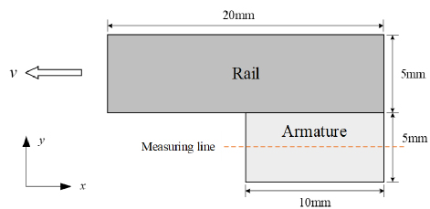
Figure 1: Computational model.
The two-dimensional electromagnetic railgun model typically exhibits symmetry. In this model, copper is chosen as the material for the rail, while the armature is made from 7075 aluminum. The armature moves along the rail in the positive direction of the x-axis at a velocity v. For the purposes of analysis, we focus on half of the armature and one side of the rail, as illustrated in Fig. 1. To simplify the calculations, we assume that the armature remains stationary while the rail moves in the negative direction of the x-axis at speed v.
B. Discretization of the magnetic diffusion equation
After derivation of Maxwell’s system of equations, the magnetic diffusion equation for the electromagnetic launcher can be expressed as [16]:
| (1) |
where t is time, U is velocity, is conductivity, B is magnetic induction and is vacuum permeability.
In this two-dimensional electromagnetic launcher model, the magnetic induction intensity in the x and y directions is neglected, and the magnetic permeability is assumed to be independent of temperature. Consequently, the magnetic diffusion equations are derived separately for the rail and the armature as follows [23]:
| (2) | |
| (3) |
where and represent the magnetic induction in the z direction experienced by the rail and the armature, respectively. Additionally, and denote the conductivity of the rail and armature, respectively.
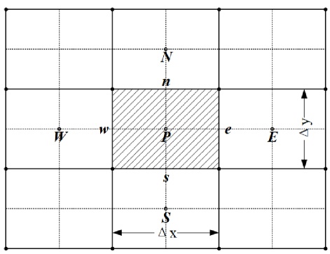
Figure 2: Finite volume method calculation grid.
The finite volume method partitions the two-dimensional computational domain of the rail cannon into control volume units, allowing for the application of conservation integrals to each unit volume [22]. Figure 2 illustrates the two-dimensional magnetic diffusion control volume grid, where point P, marked as nodes, corresponds to the control volume units. The four nodes located in the southwest, southeast, northwest, and northeast regions are represented by the points , , , and . The corresponding four unit interfaces are denoted as , , , and .
By integrating equation (2), the value of at point P can be further expressed as follows:
| (4) |
where , A is the area of the control volume and , . Control volume . The values at points , , , and are , , , and , respectively. Denoting the values of in , , , and by , , , and , respectively, equation (4) becomes:
| (5) |
The format of the implicit discrete equation that satisfies the heat conduction conditions can be expressed as follows:
| (6) |
| (7) |
For the armature, the discretized result is given by:
| (8) |
C. Discretization of the heat conduction equation
The heat conduction equation derived from Fourier’s law can be formulated as follows:
| (9) |
where is thermal conductivity, T is temperature, is density, and c is specific heat. J can be expressed as:
| (10) |
The heat transfer equations for the armature and the rail can be expressed as follows:
| (11) | |
| (12) |
Let . The discretized heat conduction equations for the rail and the armature can be formulated as:
| (15) | |
| (20) | |
| (24) |
D. Boundary conditions and simulation methods
Once the external current is applied, the magnetic fields produced by the two rails counteract each other due to their opposing current directions. In regions where the armature does not extend, no current flows, resulting in a magnetic induction intensity of 0. Within the armature, the current predominantly flows along the shortest path between the two rails, concentrating at the armature’s tail. To prevent sudden changes in the magnetic field gradient for the rails that the current has traversed, the boundary conditions for the armature’s magnetic field are established as depicted in Fig. 3. Regarding the temperature field, it is assumed that, initially, the temperature distribution within the armature is uniform at 300K, representing room temperature. It is further specified that all heat dissipates solely through internal conduction and not through the boundaries. Additionally, the normal temperature gradient along all edges is set to 0 [25].
The erosion treatment of the armature involves phase transformation, with the current focusing on the armature tail. This leads to a rapid temperature increase, causing the material to start melting upon reaching its melting point. Once the temperature surpasses the melting point it stabilizes, and any additional heat absorbed is stored. Upon reaching the latent heat of melting, the phase transition concludes, signifying the transformation of the armature into a liquid state. Following exposure to electromagnetic force, the liquid component separates from the solid armature. When the armature on the grid completely melts, assuming the molten metal separates entirely from the armature due to the high-speed armature action, the armature and the rail lose contact. The space between them is considered as air, with no current passing through the armature, resulting in a current density of zero. Consequently, the magnetic field boundary condition is then updated to reflect the unmelted region.
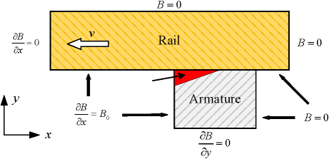
Figure 3: Setting of magnetic field boundary conditions.
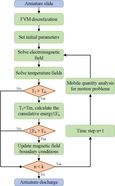
Figure 4: Overall calculation process.
The model is partitioned into 0.1 mm square grids with a time step of 0.1. The magnetic field boundary is updated using a method to simulate liquid armature separation, and the melt-wave calculation is conducted using MATLAB. The calculation process is illustrated in Fig. 4. By discretizing the magnetic diffusion and heat conduction equations for the armature and rail, these are transformed into linear equations. To calculate the steady melt-wave, initial parameters are set, maintaining the initial magnetic excitation or velocity while varying another parameter to solve for armature and rail temperatures. For the transient melt-wave calculation, the current output of each time step is computed to determine the motion characteristics and magnetic field excitation of the armature at that point. Subsequently, the magnetic field and temperature distributions are resolved using the finite volume method.
III. CALCULATIONS AND ANALYSIS
A. Calculation of steady state melt-wave
The magnetic induction intensity distribution of the armature and rail is primarily influenced by the initial magnetic field excitation and the speed of the armature, as evident from equation (1) and Fig. 3. These factors significantly impact the current density. Current density, as indicated in equation (9), plays a crucial role in altering the temperature distribution [24]. Therefore, it is essential to investigate the correlation between magnetic field excitation, armature speed, and the melt-wave. This study examines the impact of the velocity skin effect on the melt-wave and analyzes the temperature distribution of the armature with and without velocity. The erosion distance at various time points is investigated considering the influence of temperature on conductivity and compared to that under constant conductivity. The entire investigation is conducted based on 32T.
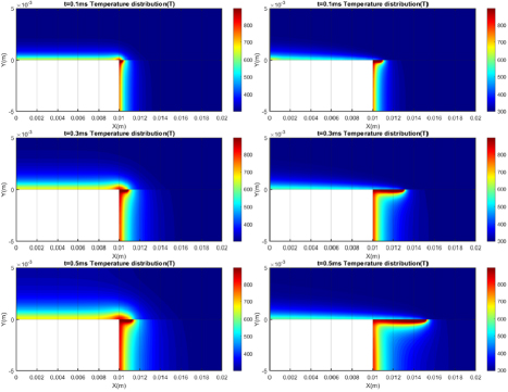
Figure 5: Comparison of melt-wave: (a) Distribution of melt-waves when the armature is at rest and (b) Distribution of melt-waves at an armature speed of 100 m/s.
Figure 5 (a) illustrates the progression of melt-waves at time intervals of 0.1 ms, 0.3 ms, and 0.5 ms with the armature speed set at 0. Initially, elevated temperatures are primarily localized at the region where the armature tail interfaces with the track. Over time, the melt-wave gradually extends towards the armature head, albeit at a relatively sluggish pace. The temperature distribution adjacent to the armature tail exhibits a wave-like pattern, diminishing towards the outer regions of the orbit.
Figure 5 (b) illustrates the propagation of melt-waves at various time points with an armature velocity of 100 m/s. In comparison to stationary armature, the melt-wave exhibits a notably broader spread over time, with armature erosion reaching 0.53 mm at 0.5 ms, whereas, at velocity, the armature erosion region forms a triangular shape, with erosion extending only to 0.13 mm at 0.5 ms. The advancement of the melt-wave at 100 m/s towards the armature head resembles a knife-like progression. This phenomenon is attributed to the speed skin effect, as depicted in Fig. 6. The rapid motion of the armature results in current concentration at the armature tail, leading to accelerated temperature rise and increased armature melting speed, thereby propelling the melt-wave towards the armature head. Consequently, the temperature distribution along the trajectory gradually decreases as the armature moves, eventually approaching room temperature (300K) at the conclusion of the melt-wave.
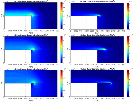
Figure 6: Comparison of current density: (a) Distribution of melt-waves when the armature is at rest and (b) Distribution of melt-waves at an armature speed of 100 m/s.
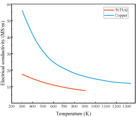
Figure 7: Conductivity-temperature curve.
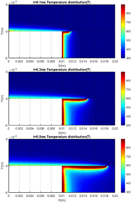
Figure 8: Melt-wave distribution of conductivity change at armature speed 100 m/s.
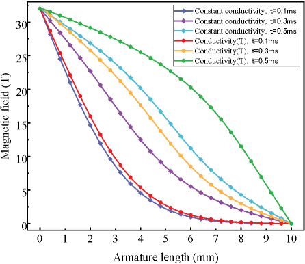
Figure 9: Magnetic flux density distribution along the measurement line under different conditions.
Figure 7 displays the conductivity-temperature profiles of 7075Al and copper, derived through data fitting based on literature [17]. Subsequently, Fig. 8 illustrates the propagation of the melt-wave at a velocity of 100 m/s corresponding to the conductivity alteration. The erosion rate is observed to be higher when conductivity changes, primarily attributed to the conductivity variation accelerating magnetic diffusion. The temporal evolution of magnetic induction intensity along the measurement line is depicted in Fig. 9. Notably, under identical conditions, the magnetic induction intensity is greater with conductivity variation compared to its absence, with the impact of conductivity alteration on magnetic diffusion intensifying over time.
Table 1: Comparison of erosion distances
| Model | Velocity of Erosion | ||
| 32T v100m/s |
40T v100m/s |
40T v150m/s |
|
| Parks [8] | 10.1m/s | 15.8m/s | 23.7m/s |
| Barber and Dreizin [18] | 8.6m/s | 13.4m/s | 20.0m/s |
| Tang et al. [11] | 7.5m/s | 12.2m/s | 18.8m/s |
| Sun et al. [13] | 6.4m/s | 13.64m/s | 16.68m/s |
| This paper (0.1 mm) |
9.9m/s | 14.8m/s | 21.1m/s |
| This paper (0.05 mm) |
9.8m/s | 14.8m/s | 21.0m/s |
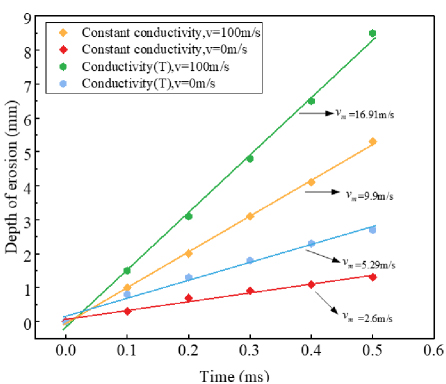
Figure 10: Comparison of erosion rates.
Table 1 displays the erosion rates calculated by the model in this study using mesh sizes of 0.05 mm and 0.1 mm, respectively, in comparison with findings from the literature [8, 11, 13, 18]. When v=100 m/s, the erosion velocities calculated by the two mesh sizes are identical. In the remaining scenarios, the erosion velocity discrepancy is a mere 0.1 mm. Given that the 0.1 mm mesh provides sufficient calculation accuracy while conserving computational resources, the results align with those of Parks and other researchers, falling within a reasonable range. Consequently, the proposed finite volume method for melting wave calculation in this study is deemed viable.
Figure 10 illustrates the correlation between melt-wave erosion depth and time under various conditions. The graph demonstrates a linear increase in erosion depth over time, with a consistent slope representing erosion velocity. This observation aligns with Parks’ conclusion in the literature [18, 19] that the erosion velocity formula is time-independent.
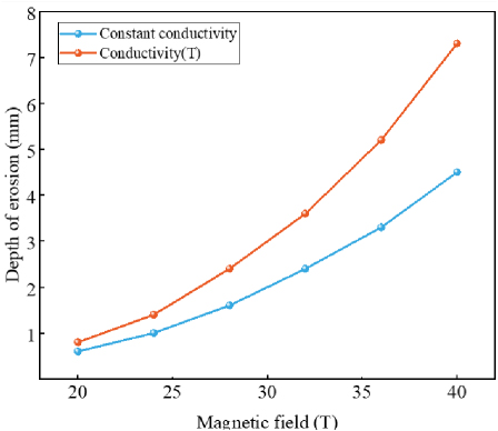
Figure 11: Erosion distance in different magnetic fields.
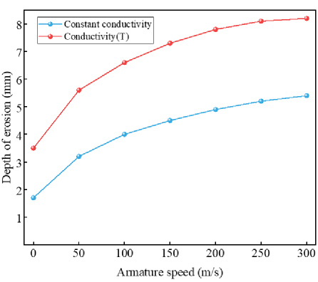
Figure 12: Erosion distance at different armature speeds.
Figure 11 illustrates a non-linear variation in erosion depth in relation to the external magnetic field excitation at 150 m/s. An increase in magnetic excitation results in a deeper penetration of the melting wave into the armature head, leading to a larger growth amplitude. The erosion distance discrepancy between conductivity change and constancy is merely 0.1 mm at 20T, whereas it escalates to 2.8 mm at 40T.
Figure 12 illustrates the impact of armature speed on erosion depth at 40T. An increase in armature speed results in a corresponding increase in erosion depth; however, this escalation gradually diminishes. With higher velocities, the disparity in melting distances between the two conditions remains relatively constant.
B. Calculation of transient melt-wave
During the actual firing process, the armature is driven by a pulsed high current, which can be expressed as follows [20]:
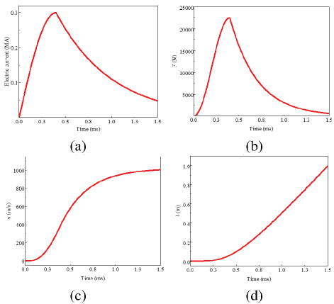
Figure 13: Current and armature motion parameter curves: (a) External pulse high current waveform, (b) Electromagnetic force curve on the armature, (c) Armature speed curve, and (d) Armature displacement curve.
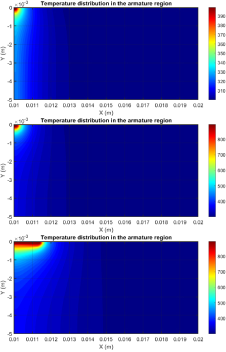
Figure 14: Distribution of armature melt-waves at different moments after current connection.
| (25) |
Given 0.3MA, 0.4 ms, 0.6 ms, and the inductance gradient is L= , the electromagnetic force F, velocity v, and the displacement l on the armature in motion can be expressed as follows [21]:
| (26) | ||
| (27) | ||
| (28) |
During the launching process, the initial excitation of the magnetic field and the speed of the armature are dictated by the external input current. Figure 13 illustrates the correlation between the external current, armature motion parameters, and time.
Figure 14 depicts the temporal evolution of armature temperature distribution at critical time instants (0.2 ms, 0.36 ms, and 0.8 ms) post current initiation. At the initial phase (t0.2 ms) corresponding to armature acceleration onset, the measured maximum localized temperature reaches 401K, remaining substantially below the bulk material’s melting threshold. The subsequent thermomechanical response reveals surface degradation initiation at t0.36 ms, characterized by incipient phase-change phenomena. Progressive joule heating culminates in a solidified melt-wave penetration depth of 1.5 mm at t0.8 ms, demonstrating time-dependent electrothermal coupling effects.
This study investigates the influence of external current on melt-wave behavior by systematically varying the peak current magnitude and its temporal profile. Figure 15 presents the time-dependent depth of erosion evolution for currents of 0.24MA, 0.30MA, and 0.36MA. As shown in Fig. 13 (a), the current initially increases before gradually decaying. Correspondingly, the melt depth in Fig. 15 exhibits an initial growth phase followed by stabilization after 1 ms, resulting from a dynamic equilibrium between increasing armature velocity and decreasing current density. Post-stabilization depth of erosion stabilizes at 0.5 mm, 1.7 mm, and 3.2 mm for 0.24MA, 0.30MA, and 0.36MA, respectively, indicating significant suppression of thermal erosion with current reduction. However, excessive current reduction compromises armature muzzle velocity, limiting practical applicability. Comparison with literature [13] confirms consistent temporal trends and maximum depth of erosion (1.7 mm) at 0.30MA, validating the experimental methodology.
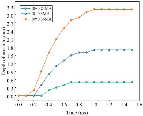
Figure 15: Distance of erosion at different peak currents.
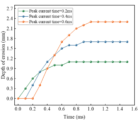
Figure 16: Erosion distance for different rise times.
The concurrent increase in current and armature velocity synergistically enhances thermal erosion. Figure 16 demonstrates that shorter armature acceleration durations correlate with earlier erosion initiation and reduced stabilization distances. This correlation arises because rapid current rise rates intensify instantaneous joule heating, accelerating phase-change processes. As evidenced in Fig. 15, an optimization strategy involves elevating current amplitude while compressing rise time to minimize melt formation without compromising armature launch precision. This approach leverages the competing effects of enhanced electromagnetic propulsion and reduced thermal exposure duration.
IV. CONCLUSION
The penetration of the melt-wave through the armature surface creates a significant gap between the armature and the rail, leading to armature transition. Therefore, this paper proposes, for the first time, a two-dimensional numerical model of the melt-wave in electromagnetic railgun launches based on the finite volume method. By comparing the results with those from four previous studies, the model demonstrates consistency, confirming the applicability of the finite volume method for investigating armature characteristics in electromagnetic railgun systems.
Steady-state calculations of the melt-wave reveal that high temperatures initially concentrate at the armature tail and propagate toward the head, driven by the velocity skin effect. Under constant conditions, the erosion distance increases linearly over time. When considering the temperature dependence of electrical conductivity, the erosion distance increases more significantly. Additionally, increases in initial magnetic excitation and armature velocity also lead to greater erosion distances.
Upon applying an external current, changes in initial magnetic excitation and armature velocity are determined by the current waveform. As the launch time increases, the erosion distance initially rises sharply before stabilizing. Reducing the current rise time or magnitude effectively inhibits the progression of erosion.
This study provides a theoretical foundation for improving the launch lifespan of electromagnetic railguns. To better approximate real-world launch conditions, future research should consider the effects of non-ideal contact on armature melting.
REFERENCES
[1] J. Lydia, R. Karpagam, and R. Murugan, “A novel technique for dynamic analysis of an electromagnetic rail launcher using FEM coupled with Simplorer,” Applied Computational Electromagnetics Society (ACES) Journal, vol. 37, pp. 229-237, 2022.
[2] J. Zhang, J. Lu, S. Tan, B. Li, and Y. Zhang, “Research status of surface damage in rails for electromagnetic launchers,” Acta Armamentarii, vol. 44, pp. 1908-1919, 2023.
[3] X. Wan, J. Lu, D. Liang, and J. Lou, “Thermal analysis in electromagnetic rail launcher taking friction heat into account under active cooling condition,” IEEE Access, vol. 8, pp. 84720-84740, 2020.
[4] B. Gu and C. Yang, “A review of the computational investigation of three-dimensional transient magneto-thermal coupling characteristics of electromagnetic railgun armature and rail in high-speed sliding electrical contact,” J. Phys.: Conf. Ser., vol. 2478, no. 8, p. 082016, June 2023.
[5] S. Ren, G. Feng, and S. Liu, “Study on wear of electromagnetic railgun,” IEEE Access, vol. 10, pp. 100955-100963, 2022.
[6] S. Ma, S. Lu, H. Ma, H. Wang, A. Nong, D. Ma, C. Yan, and C. Liu, “Investigation on the spatial-temporal distribution of electromagnetic gun rail temperature in single and continuous launch modes,” IEEE Trans. Plasma Sci, vol. 50, pp. 2270-2278, July 2022.
[7] L. Chen, X. Xu, Z. Wang, J. Xu, P. You, and X. Lan, “Melting distribution of armature in electromagnetic rail launcher,” IEEE Trans. Plasma Sci, vol. 51, pp. 234-242, Jan. 2023.
[8] P. B. Parks, “Current melt-wave model for transitioning solid armature,” Journal of Applied Physics, vol. 67, no. 7, pp. 3511-3516, Apr. 1990.
[9] F. Stefani, R. Merrill, and T. Watt, “Finite element analysis of melt wave ablation in electromagnetic rail launcher armatures,” IEEE Trans. Magn., vol. 41, no. 1, pp. 437-441, Jan. 2005.
[10] F. Gong. “Study of erosion mechanism at the armature-rail contact interface in railgun,” Thesis, Nanjing University of Science and Technology, Nanjing, Jiangsu, China, 2014.
[11] B. Tang, Y. Xu, Q. Lin, and B. Li, “Synergy of melt-wave and electromagnetic force on the transition mechanism in electromagnetic launch”, IEEE Trans. Plasma Sci, vol. 45, pp. 1361-1367, July 2017.
[12] S. Tan, J. Lu, X. Zhang, X. Guan, and X. Long, “Two-dimensional numerical simulation of melt-wave erosion in solid armatures,” J. Xi’an Jiaotong Uni., vol. 50, no. 3, pp. 106-111, Mar. 2016.
[13] J. Sun, J. Cheng, Q. Wang, L. Xiong, Y. Cong, and Y. Wang, “Numerical simulation of melt-wave erosion in 2-D solid armature,” IEEE Trans. Plasma Sci., vol. 50, no. 4, pp. 1032-1039, Apr.2022.
[14] J. Cen and Q. Zou, “Deep finite volume method for partial differential equations,” Journal of Computational Physics, vol. 517, p. 113307, July2024.
[15] B. Li, J. Lu, S. Tan, Y. Jiang, and Y. Zhang, “Application of finite volume method in analyzing sliding electrical contact problem,” Journal of Naval Univ. of Engineering, vol. 31, no. 6, pp. 23-28, Dec.2019.
[16] Y. Yang, Q. Yin, C. Li, H. Li, and H. Zhang, “Simulation and experimental verification of magnetic field diffusion at the launch load during electromagnetic launch,” Sensors, vol. 23, no. 18, p. 8007, 2023.
[17] K. T. Hsieh and B. K. Kim, “International railgun modelling effort,” IEEE Trans. Magn., vol. 33, no. 1, pp. 245-248, Jan. 1997.
[18] J. P. Barber and Y. A. Dreizin, “Model of contact transitioning with ‘realistic’ armature-rail interface,” IEEE Trans. Magn., vol. 31, no. 1, pp. 96-100, Jan. 1995.
[19] T. Watt and F. Stefani, “The effect of current and speed on perimeter erosion in recovered armatures,” IEEE Trans. Magn., vol. 41, no. 1, pp. 448-452, Jan. 2005.
[20] J. D. Powell and B. K. Kim, “Observation and simulation of solid armature railgun performance,” IEEE Trans. Magn., vol. 24, no. 1, pp. 84-89, Jan. 1999.
[21] A. Guo, X. Du, X. Wang, and S. Liu, “Calculation of armature melting wear rate based on contact surface heat distribution,” IEEE Trans. Plasma Sci., vol. 51, no. 7, pp. 2981-2990, July 2024.
[22] C.-C. Wu, D. Völker, S. Weisbrich, and F. Neitzel, “The finite volume method in the context of the finite element method,” Materials Today: Proceedings, vol. 62, pp. 2679-2683, 2022.
[23] G. Liao, W. Wang, B. Wang, Q. Chen, and X. Liu, “Transient mixed-lubrication and contact behavior analysis of metal liquid film under magneto-thermal effect,” International Journal of Mechanical Sciences, vol. 271, p. 109142, June 2024.
[24] J. Yao, L. Chen, S. Xia, J. He, and C. Li, “The effect of current and speed on melt erosion at rail-armature contact in railgun,” IEEE Trans. Plasma Sci., vol. 47, no. 5, pp. 2302-2308, May 2019.
[25] G. Fei and W. Chunsheng, “Two-dimensional numerical simulation of melt-wave erosion in solid armatures,” J. Nanjing Univ. Sci. Technol., vol. 36, no. 3, pp. 487-491, 2012.
BIOGRAPHIES

Kefeng Yangreceived the B.S. degree in weapons launch engineering from Air Force Engineering University, Xi’an, China, in 2023. He is currently a graduate student in mechanics at Air Force Engineering University, where his interests include theory and technology of weapon systems, especially about the electromagnetic launch technology.

Gang Feng received the M.S. degree in weapons from Air Force Engineering University, Xi’an, China. He is currently a Professor at the Air and Missile Defense College, Air

Shaowei Liu received the B.S. and Ph.D. degrees in weapons from the Air Force Engineering University, Xi’an, China, in 2005 and 2008, respectively. He is currently an Associate Professor at the Air Defense and Anti-Missile School, Air Force Engineering University. His current research interests include the theory and technology of weapon systems.

Xiaoquan Lu received the B.S. degree in weapons launch engineering from Air Force Engineering University, Xi’an, China, in 2022. He is currently a graduate student in mechanics at Air Force Engineering University, where his interests include theory and technology of weapon systems.

Xiangyu Du received the B.S. degree in weapons in 2020 and the M.S. degree in mechanics in 2023 from the Air Force Engineering University, Xi’an, China, where he is currently pursuing the Ph.D. degree in weapons. His current research interests include theory and technology of weapon systems, especially about electromagnetic launch technology.

Tianyou Zheng received the B.S. degree in weapons launch engineering from Air Force Engineering University, Xi’an, China, in 2023. He is currently a graduate student in mechanics at Air Force Engineering University, where his interests include contact characteristics of railguns under pulsed high current conditions.
ACES JOURNAL, Vol. 40, No. 8, 745–754
doi: 10.13052/2024.ACES.J.400807
© 2025 River Publishers