Space and Frequency Extrapolation for Deep Learning Design of Coupling Matrix for Microwave Filters

Tarek Sallam and Qun Wang

School of Computer Science and Technology Shandong Xiehe University, Jinan 250109, Shandong, China
tarek.sallam@feng.bu.edu.eg

Submitted On: January 22, 2025; Accepted On: January 25, 2026

ABSTRACT

In this paper, we propose a deep-learning-based neural network namely, a convolutional neural network (CNN) for predicting frequency response of a microwave filter as a function of its extrapolated coupling parameters. Thus, in this paper, coupling properties of a microwave filter comprise its design space. This space characterizes the filter’s frequency response in complex domain. Moreover, we propose a CNN-based method to extrapolate the response in frequency. Thereby, excessive simulations and long computational time can be avoided as opposed to electromagnetic (EM) solvers. The training of the proposed CNN is based on a circuit model. In order to exhibit the robustness of the new technique, it is applied on 5- and 8-pole filters and compared with a shallow neural network namely, radial basis function neural network (RBFNN). The results reveal that the CNN can achieve extrapolation in both design space and frequency for microwave filters with high accuracy and speed. For a 5-pole filter, the percentage root mean square error (RMSE) between ideal and predicted response of CNN is found to be 0.28% and 0.09% for design space exploration (DSE) and frequency extrapolation (FE), respectively. For an 8-pole filter, the percentage RMSE of CNN is found to be 0.38% and 0.11% for DSE and FE, respectively.

Keywords: Convolutional neural network (CNN), coupling matrix, deep learning, microwave filters, radial basis function neural network (RBFNN).

1 INTRODUCTION

Microwave filters are widely used in all types of electronic systems [1, 2]. Tuning of microwave filters is an inevitable process in the design procedure of microwave filters. For the case of coupled resonator filters, either computing $S$ -parameters for a given coupling matrix or extracting the coupling matrix from the required $S$ -parameters is a crucial problem. Solving either problem becomes extremely difficult since it is a highly nonlinear problem [3, 4]. Classical methods dealt with problem need to be repeated for many iterations in different conditions [5, 6]. Consequently, the process of filter design suffers from the time-consuming and complicated parameters extraction.

Some conventional (shallow or non-deep) Neural network (NN) techniques were developed for microwave filter modeling [7, 8, 9, 10, 11, 12]. However, these techniques are not suitable for high-dimensional problems because data generation and model training become too complicated. Deep learning (DL)-based methods were also proposed for microwave filter design and modeling [13, 14]. However, in these methods, the training data is generated using full-wave electromagnetic (EM) model through simulation or measurement which becomes impractical when large training data is needed. Therefore, collection of training data using EM-based models to cover input/output parameter range over the interested frequency band can be an overwhelmingly time-consuming task. Different from EM models, circuit models can be used to introduce fast accurate models for different electronic designs. They are usually straightforward to build, and fast to evaluate. In [15], a convolutional neural network (CNN) [16, 17], a variant of deep network framework, is used to extract the coupling matrix of ideal (target) $S$ -parameters based on a circuit model. The CNN first extracts the features of $S$ -parameters by using convolution layers and pooling layers, which are then mapped to the coupling matrix by full connection and output layers.

Microwave filters can be designed by using EM solvers to obtain their frequency responses. While a full-wave EM simulation is accurate, it solves complex equations iteratively to compute the frequency response of the structure. This makes the simulation utilize a high amount of computational resource and time because of the high dimensionality of input space. Given a frequency response of the filter for a certain input design, it is often necessary to have information about out-of-bound design space response. In a traditional way, it may be required to perform EM simulations again. This makes design space exploration (DSE) of microwave filters indispensable.

Initial DSE techniques involved statistically derived design-of-experiment (DoE) analysis [18, 19]. However, these methods do not cope well with the increasing dimensionality and nonlinearity of design spaces [20, 21]. To address these limitations, evolutionary algorithms for DSE were developed [22, 23]. The advantage with evolutionary techniques is that they made no assumptions about the nature of the design space. However, they often require a large number of function evaluations and convergence rates are problem-dependent leading to long computation times [24, 25]. In [26], the authors provide a machine learning (ML)-based architecture that accomplishes DSE with high accuracy for microwave and RF components. However, this architecture requires long training and execution times compared to DL-based techniques.

In most scenarios, only band-limited data is available because broadband data might be computationally expensive to be simulated or measured. Therefore, extrapolation along the frequency axis or frequency extrapolation (FE) becomes a compelling concept because it enables us to estimate the frequency response over a larger range without performing extra measurements or simulations. Although FE has been discussed in the past [27, 28, 29, 30, 31, 32, 33, 34, 35, 36], these approaches only deal with responses with few resonant frequencies and fail to deal with responses having multiple resonant peaks and dips. Knowledge-based NNs are used in [37] to provide extrapolated results for the design space parameters for microwave modeling and design. While this approach works for DSE, it may not be applicable to FE. In [38], a Hilbert-based long short-term memory recurrent neural networks (HilbertNet) architecture is proposed to extrapolate the frequency response of EM structures. The problem with HilbertNet is that it consumes a long training time, besides it becomes less confident with less training data and in predictions where the frequency points are far off from the cutoff frequency.

DL-based approaches [39] overcome several of the aforementioned challenges: they can be applied to predict complex responses covering much larger design spaces, and it can predict output response in far less computational time, in either training or execution, than traditional methods. In this paper, the DL-based approach used in [15], namely CNN, is extended to accomplish extrapolation in both DSE and FE for microwave filters. To validate the effectiveness of the proposed CNN, it is applied on 5- and 8-pole microwave filters. The proposed CNN model is able to predict the frequency response in either DSE or FE with high accuracy and speed (in both training and execution) compared with a radial basis function neural network (RBFNN) [40, 41, 42, 43] which is a shallow (non-deep) NN.

2 CNN FOR CIRCUIT MODEL-BASED DSE AND FE

The circuit model-based equation that relate the coupling matrix $M$ and filter $S$ -parameters is given by [44]:

$S_{11}$	$= 1 + 2 j R_{1} {[γ I - j R + M]}_{11}^{- 1}$
$S_{21}$	$= - 2 j \sqrt{R_{1} R_{2}} {[γ I - j R + M]}_{N 1}^{- 1},$	(1)

where $γ = (f_{0} / B W) ((f / f_{0}) - (f_{0} / f))$ , $f, f_{0}$ , and BW are the frequency, filter center frequency, and filter bandwidth, respectively, N is the filter order, I is $N \times N$ identity matrix, M is the $N \times N$ symmetric coupling matrix, R is a $N \times N$ matrix with all entries are zero except ${[R]}_{11} = R_{1}$ and ${[R]}_{N N} = R_{2}$ , and $R_{1}$ and $R_{2}$ are the filter’s input and output coupling parameters, respectively, as shown in Fig. 1 [44].

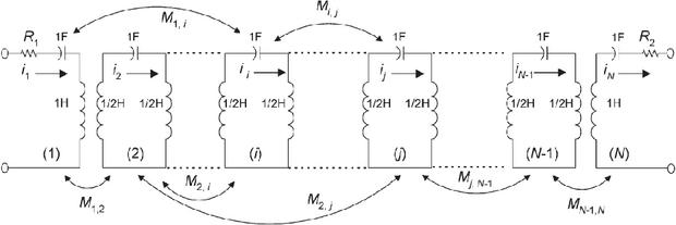
Figure 1 Equivalent circuit of an N-coupled resonator filter.

2.1 Design space exploration

The CNN model for DSE, shown in Fig. 2 (a), uses forward mapping. The input of the CNN is the vector of nonzero coupling parameters $M_{n z}$ . The output of the CNN is the required vectors $| S_{11} |$ and $| S_{21} |$ , representing the scalar magnitudes of the two $S$ -parameters at $ℛ_{DSE}$ frequency points in the full frequency range of interest. Therefore, the total number of outputs is $2 ℛ_{D S E}$ . In the case of DSE, the number of the frequency points $ℛ_{D S E} = 2001$ .

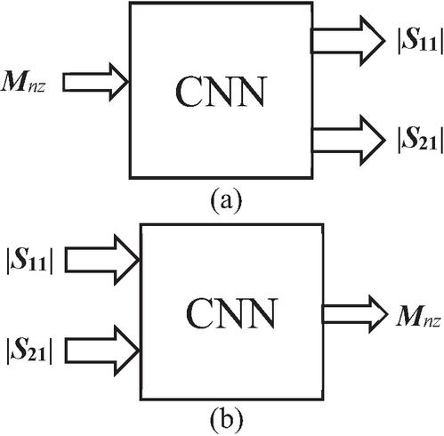
Figure 2 Circuit model-based CNN for coupling matrix extraction: (a) design space exploration (DSE) and (b) frequency extrapolation (FE).

In order to generate the training and validation data of CNN, we assume a training space for every ideal nonzero coupling parameter. Here, the assumed training space is composed of two ranges: [ $M_{nz}^{ideal} - 1.5, M_{nz}^{ideal} - 0.5]$ and $[M_{n z}^{ideal} + 0.5, M_{nz}^{ideal} + 1.5]$ , where $M_{n z}^{ideal}$ is the vector of ideal nonzero coupling parameters. 1.5 and 0.5 are two vectors of the same length as $M_{n z}^{ideal}$ and whose all elements are 1.5 and 0.5, respectively. We then use 12500 (10000 for training and 2500 for validation) uniformly distributed random samples in this space for coupling parameters. For each sample of coupling parameters, (2) is used to obtain the corresponding $S$ -parameters. In this way, we can get the training and validation data for the DSE model. Once trained, the frequency response of an input coupling tuple is predicted, which is beyond the bounds of the training space, namely, the extrapolation coupling tuple. In this case, the extrapolation coupling tuple is the vector of ideal nonzero coupling parameters $M_{n z}^{ideal}$ . Then, the predicted frequency response is compared to the ideal one. The accuracy of the predicted frequency response for the extrapolated coupling tuple is a measure of the generalization capability of the network.

2.2 Frequency extrapolation

Extrapolating the frequency response is important since designers need to determine if there are any resonances in proximity to the simulated (or measured) data which are bandlimited. The CNN model for FE, shown in Fig. 2 (b), uses what so called inverse mapping. In contrast with DSE model, the input of the FE model is the vectors $| S_{11} |$ and $| S_{21} |$ at $ℛ_{F E}$ frequency points along only a half of the frequency range of interest. The model is trained along the first half of the frequency range while extrapolated (tested) along the second half. In either case, $ℛ_{F E}$ is 1001 frequency points, thus the total input is $2 ℛ_{F E} = 2002$ . The output of the CNN is the vector of nonzero coupling parameters $M_{n z}$ .

In order to generate the training and validation data of CNN, we assume a tolerance of $\pm$ 0.5 for every ideal nonzero coupling parameter. We then use 12500 (10000 for training and 2500 for validation) uniformly distributed random samples in this range for coupling parameters. For each sample of coupling parameters, (2) is used to obtain the corresponding $S$ -parameters along the training frequency range. By swapping the data of coupling parameters and $S$ -parameters, we can get the training and validation data for the FE model. The trained CNN is tested by the ideal set of $S$ -parameters (corresponding to the ideal $M_{n z}$ ) along the extrapolated frequency range. Then, the extrapolated (predicted) frequency response is compared to the ideal one. It should be noted that the layouts for DSE and FE, shown in Figs. 2 (a) and (b), have proved their efficacy [26]. This also will be seen throughout the results in the paper.

3 PROPOSED STRUCTURES

3.1 RBFNN model

RBFNN is a special three-layer feedforward network, which consists of an input layer, an output layer, and a single hidden layer as shown in Fig. 3. In the hidden layer, the nonlinear functions are usually considered to be Gaussian functions of appropriately chosen means and variance. The weights from the hidden to the output layer are determined by considering a supervised learning procedure. Assume that the input, hidden, and the output layers have J, K, P nodes, respectively. The network output vector is given by

w_{p} = \sum_{k = 1}^{K} ω_{p, k} e^{- \frac{{‖ z - c_{k} ‖}^{2}}{σ_{k}^{2}}} (p = 1, \dots, P),

(2)

where $z = [z_{1} z_{2} \dots z_{J}]$ is the input vector, $c_{k}$ and $σ_{k}$ are the center vector and the standard deviation (spread parameter) of the $k^{th}$ Gaussian function, respectively, and ${ω_{p, k}; p = 1, \dots, P; k = 1, \dots, K}$ is the weight from the $k^{th}$ hidden node to $p^{th}$ output node.

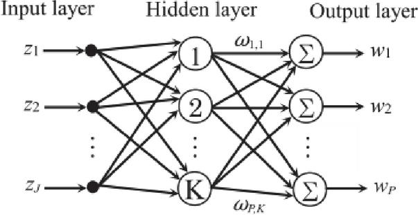
Figure 3 Architecture of the RBFNN.

3.2 CNN model

CNNs have one or more convolutional and pooling layers to learn the discriminative features from the input data. After all the convolutional and pooling layers, these learned features are then aggregated to the vectors by the fully connected layers for the regression task [45]. After many simulation trials, it is found that the CNN structures for DSE and FE which provide the best accuracy and ensure optimal network performance are detailed in Table 1. There are three convolutional (Conv) layers and three maximum pooling (MaxPool) layers. The number of feature maps at each convolutional layer is as twice as the previous layer. Each convolutional layer is followed by a pooling layer to reduce the dimension of network parameters. All convolutional layers have a stride of 1 and ‘same’ padding. All pooling layers have a size of $2 \times 2$ , stride 2, and ‘same’ padding. After the sequence of convolutional and pooling layers, there is a single fully connected (FC) layer followed by the output layer. In order to avoid overfitting during training, a dropout operation with a rate of 50% is used at the end of the convolutional and pooling layers. The activation functions used in the convolutional layers and the fully connected layer are rectified linear unit (ReLU) and exponential linear unit (ELU), respectively. Since this is a regression problem instead of a classification problem, no activation is used at the output layer (linear activation).

Table 1 Proposed CNN structures for DSE and FE

Layer	Size		Nodes		Stride		Padding		Activation
	FE	DSE	FE	DSE	FE	DSE	FE	DSE	FE	DSE
Input (Image)	$-$		$1 \times 2 \times 1001 = 2002$	$1 \times 1 \times Length {M_{n z}} = Length {M_{n z}}$	$-$		$-$		$-$
Conv1	$2 \times 2$	$3 \times 3$	8	64	1		same		ReLU
MaxPool1		$2 \times 2$	$-$		2				$-$
Conv2		3 $\times$ 3	16	128	1				ReLU
MaxPool2		2 $\times$ 2	$-$		2				$-$
Conv3		3 $\times$ 3	32	256	1				ReLU
MaxPool3		2 $\times$ 2	$-$		2				$-$
50% Dropout
FC	$-$		50	500	$-$		$-$		ELU
Output	$-$		$Length {M_{n z}}$	4002	$-$		$-$		Linear

For DSE structure, the input vector is first reshaped into a $1 \times 1 \times Length {M_{n z}}$ input image. The first convolutional layer comprises of 64 feature maps. There are 128 and 256 feature maps in the second and third layers, respectively. The size of the feature map in each convolutional layer is fixed at $3 \times 3$ . The FC layer has 500 nodes. The output layer has $2 ℛ_{D S E} = 4002$ nodes.

The FE model is used to predict the frequency response over only half of the frequency range of interest. Its structure is simpler than that of the DSE, as shown in Table 1. First, its total 2002 inputs are reshaped into a $1 \times 2 \times 1001$ input image. The three convolutional layers have 8, 16, and 32 feature maps, respectively. The size of the feature map in any convolutional layer is fixed at $2 \times 2$ . The FC layer has 50 nodes. The output layer has a number of nodes equals the number of nonzero coupling parameters. It should be noted that RBFNN has the same number of inputs and output as the CNN except it cannot accept an image or 2D input. Therefore, the input vector in this case is 1D.

4 EXAMPLES

To verify the performance of the CNN-based DSE and FE models, they are applied on 5- and 8-pole microwave filters. The Adam (adaptive momentum) optimization algorithm [46] is used to update the network weights and the loss function used for this network is the mean squared error. The initial value of the learning rate is 0.001. During the training, the learning rate is decreased by a rate of 0.1 each 40% of number of epochs. The batch size is 40 and number of epochs is 10. To further verify the performance of the CNN, it is compared to that of the RBFNN. In all examples, the filter’s input and output coupling parameters are assumed to be equal, i.e., $R_{1} = R_{2}$ . The CNN is implemented (trained, validated, tested) using MATLAB R2024a using Deep Learning Toolbox. The RBFNN is trained using the training function “newrb” in the same toolbox, in which a hidden node is added each epoch (iteration) until a target mean square error (MSE) is reached.

4.1 5-pole filter

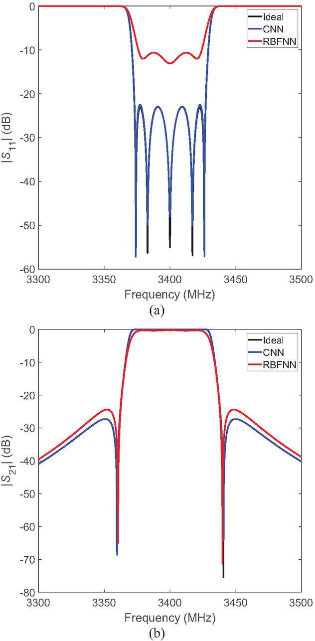
In this example, we use the proposed CNN to develop DSE and FE models for a 5-pole dielectric resonator filter with a 3.4 GHz center frequency and a 54 MHz bandwidth [44]. The nonzero coupling parameters are $M_{n z} = {[R_{1} M_{12} M_{14} M_{23} M_{34} M_{45}]}^{T}$ with their ideal values $M_{n z}^{ideal} = [1.1330, 0.8660, - 0.2520, 0.7920$ , $0.5950, 0.9010]^{T}$ .

Figure 4 DSE responses of a 5-pole filter: (a) return loss and (b) insertion loss.

Figure 4 shows the DSE predicted frequency responses of CNN and RBFNN compared to the ideal one. As can be seen, there is a perfect agreement between the ideal and CNN responses compared with the RBFNN response, that is, owing to the capability of CNN to extract the hidden features in the input data, automatically. On the other hand, because the RBFNN is shallow, it cannot strengthen the network training process by reconstructing the input coupling parameters. The used shallow RBFNN, has only one hidden layer with 200 neurons, cannot represent this high-dimensional input-output relationship effectively. Our proposed CNN modeling technique is suitable for this high-dimensional modeling problem. The training and validation losses of CNN for DSE are found to be 0.0358 and 0.0319, respectively.

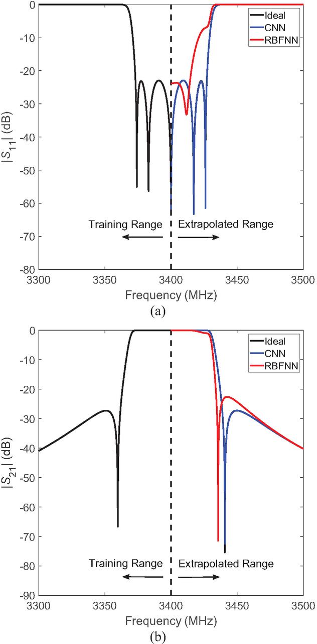
Figure 5 FE responses of a 5-pole filter: (a) return loss and (b) insertion loss.

Figure 5 shows the corresponding FE responses. As shown, the CNN and RBFNN are trained only on the first half of the response to extrapolate the second half. As can be seen, the extrapolated CNN response exactly follows the ideal one compared to RBFNN which is away from accuracy. In general, conventional shallow NNs cannot extrapolate. This is because they are meant to create a mapping from the input function space to output function space. Given an input testing point way beyond the training range, the network is highly prone to errors depending on whether it is overfitting or underfitting the data. The training and validation losses of CNN for FE are found to be 0.3030 and 0.2914, respectively.

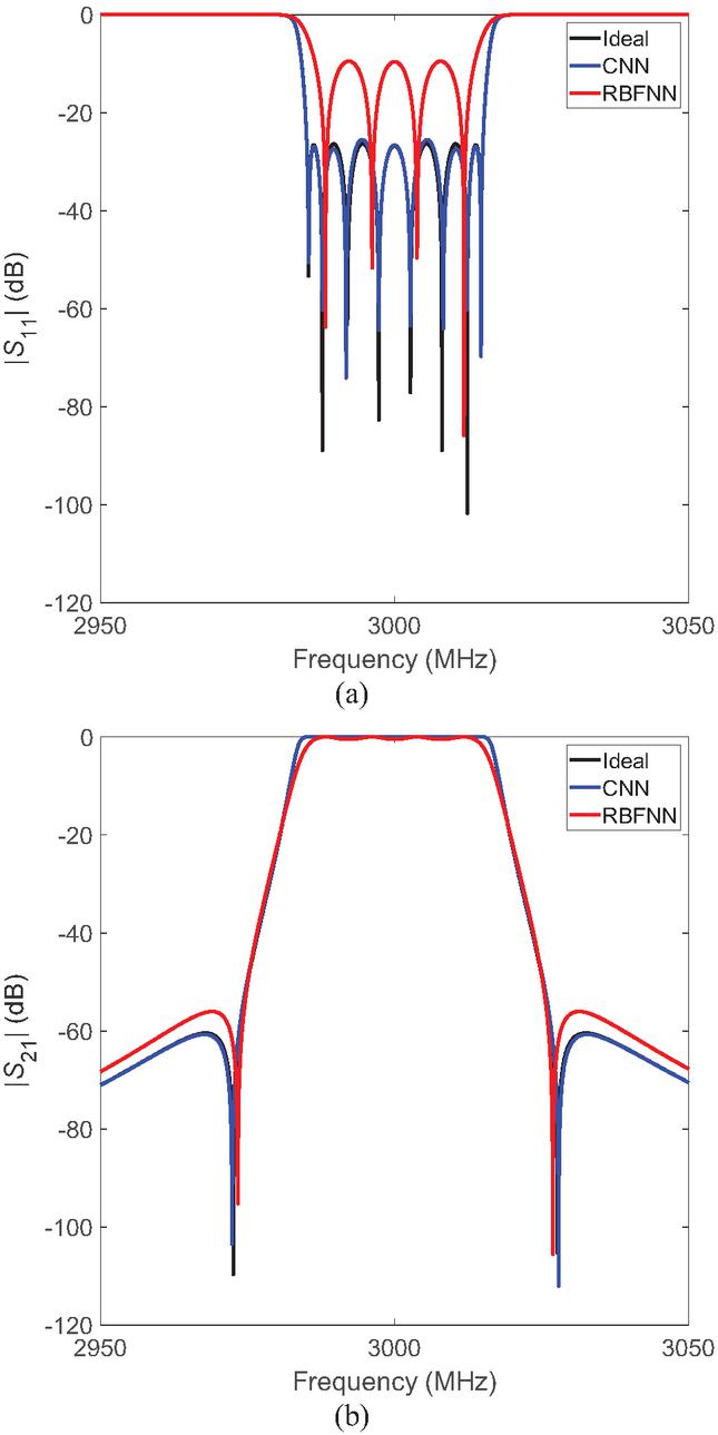
Figure 6 DSE responses of an 8-pole filter: (a) return loss and (b) insertion loss.

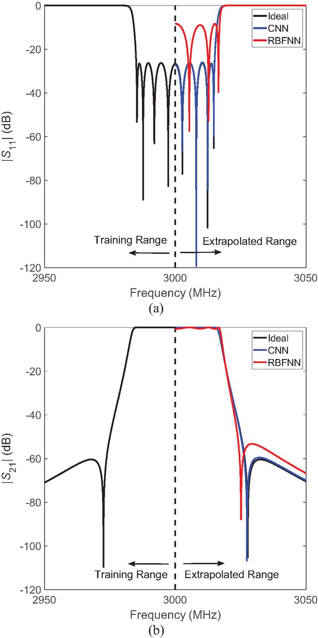
Figure 7 FE responses of an 8-pole filter: (a) return loss and (b) insertion loss.

4.2 8-pole filter

The second example involves the DSE and FE of an 8-pole elliptic-function filter with 30 MHz bandwidth centered at 3 GHz [47]. The nonzero couplings are $R_{1}$ , $M_{12}$ , $M_{23}$ , $M_{27}$ , $M_{34}$ , $M_{36}$ , $M_{45}$ , $M_{56}$ , $M_{67}$ , $M_{78}$ . However, the coupling matrix of this filter is dual-symmetrical meaning that it is symmetrical with respect to its anti-diagonal as well as its diagonal [48]. Therefore, $M_{12} = M_{78}$ , $M_{23} = M_{67}$ , and $M_{34} = M_{56}$ . Consequently, the output of NNs is $M_{n z} = {[R_{1} M_{12} M_{23} M_{27} M_{34} M_{36} M_{45}]}^{T}$ . The ideal values are

M_{n z}^{ideal} = {[\begin{matrix} 1.2420, 0.9380, 0.6310, - 0.0180, \\ 0.5760, 0.0660, 0.5190 \end{matrix}]}^{T}

Table 2 Percentage RMSE, training, and execution times of CNN and RBFNN for DSE and FE for 5- and 8-pole filters

NN	5-Pole Filter			8-Pole Filter
	Training Time	Execution Time	RMSE (%)	Training Time	Execution Time	RMSE (%)
DSE
CNN	6.2 min	0.05 s	0.28	6.35 min	0.06 s	0.38
RBFNN	2.9 h (200 hidden neurons)	1.4 s	14.72	7.1 h (400 hidden neurons)	1.7 s	16.85
FE
CNN	34 s	0.04 s	0.09	35 s	0.05 s	0.11
RBFNN	1.8 h (150 hidden neurons)	0.14 s	13.8	3.2 h (350 hidden neurons)	0.19 s	15.81

The predicted DSE and FE $S$ -parameters by both NNs along with the ideal ones are shown in Figs. 6 and 7, respectively. As shown in Figs. 6 (a) and 7 (a), the CNN captures all the resonant peaks and dips along passband with very high accuracy in contrast with RBFNN. In general, there is excellent correlation between the ideal and CNN responses, compared to RBFNN. The RBFNN architecture fails to learn the frequency response because of a lack of learning data dependencies. This shows that CNN architecture allows for parameter sharing and exploitation of spatial dependencies in data to learn a complex frequency response. We conclude that the CNN is much more accurate than the RBFNN for DSE and FE of microwave filters. The CNN training and validation losses for DSE are found to be 0.0227 and 0.0169, while they are 0.2843 and 0.2913 for FE, respectively.

Table 2 shows the training and execution times as well as the percentage root mean square error (RMSE) between ideal and predicted responses by NNs for DSE and FE for 5- and 8-pole filters. Table 2 also shows the number of hidden neurons in the hidden layer of RBFNN for each response. It can be seen that the CNN modeling for either DSE or FE is with much higher accuracy and much shorter training and execution times than the RBFNN modeling. As mentioned earlier, the RBFNN is a shallow type NN (only has one hidden layer whatever the number of hidden neurons used). That is why it takes much longer training time when dealing with high-dimensional problems (like the present one). On the other hand, the DL-based CNN can retrieve features from data with high dimensions with much shorter training and execution times due to its sparse connectivity and shared weights enabling CNNs to have small numbers of parameters.

Since FE structure, in general, is simpler than the DSE structure, it has less error and shorter training and execution times than those of DSE. Also, compared to a 5-pole filter, the 8-pole filter has higher error and higher training and execution times whether for DSE or FE, because it has a more complex frequency response than that of a 5-pole filter.

For CNN, the training data generation times of a 5-pole filter for DSE and FE are 2.4 min and 1.6 min, respectively. For an 8-pole filter, they are 2.7 min and 2.1 min, respectively. This indicates that the full time required to achieve a result from a trained CNN network for either filter (including the dataset generation) is still very small compared with the time required to achieve the same result in a classical way using direct models. Moreover, our proposed circuit model-based CNN can provide extrapolation results instantly (its execution time is a fraction of a second as shown in Table 2), while the classical full-wave EM model-based methods can take hours to do that by repetitively simulating/measuring the filter during optimization iterations. Although a large training dataset may be required for network training, it can be implemented offline. After training, it can be used online (in the execution phase) for DSE and FE of microwave filters. In other words, the network training (including the dataset generation) is done only once after that the network can be used as a real-time design space and frequency extrapolator for microwave filters.

5 CONCLUSION

A circuit model-based CNN is proposed for design space and frequency extrapolation of microwave filters. In this paper, the coupling parameters of microwave filter constitute its design space. The CNN-based approach is used to predict the frequency response as a function of the coupling properties. The results show that the proposed CNN method can be used reliably to perform the DSE and FE for microwave filters. Compared to the shallow neural network, the deep-learning-based CNN is much more accurate and faster whether in training or execution. Unlike the full-wave EM model-based methods, our proposed CNN model does not need to simulate and/or measure the filter iteratively, therefore saving much computational time and resources. For a 5-pole filter, the training time of CNN is found to be 6.2 min and 34 s for DSE and FE, respectively. For an 8-pole filter, the training time of CNN is found to be 6.35 min and 35 s for DSE and FE, respectively. In general, the execution time of CNN is a fraction of second. The CNN training and validation losses are found to be comparable indicating that CNN is not overtrained. Once the CNN model is developed (trained and validated), it can be utilized as an instant design space and frequency extrapolator for microwave filters for similar tasks, i.e., it can be used for design space and frequency extrapolation for any N-pole filter.

REFERENCES

[1] R. J. Cameron, C. M. Kudsia, and R. T. Mansour, Microwave Filters for Systems: Fundamentals, Design and Applications. Hoboken, NJ: Wiley, 2018.

[2] S. Saleh, W. Ismail, I. S. Z. Abidin, and M. H. Jamaluddin, “Compact 5G hairpin bandpass filter using non-uniform transmission lines theory,” Applied Computational Electromagnetics Society (ACES) Journal, vol. 36, no. 2, pp. 126–131, Feb. 2021.

[3] L. Accatino, “Computer-aided tuning of microwave filters,” in IEEE MTT-S Int. Microw. Symp. Dig., pp. 249–252, June 1986.

[4] M. Yu and W. C. Tang, “A fully automated filter tuning robots for wireless base station diplexers,” in Proc. Workshop, Comput. Aided Filter Tuning, IEEE Int. Microw. Symp., Philadelphia, PA, pp. 8–13, June 2003.

[5] G. Macchiarella and D. Traina, “A formulation of the Cauchy method suitable for the synthesis of lossless circuit models of microwave filters from Lossy measurements,” IEEE Microw. Wireless Compon. Lett., vol. 16, no. 5, pp. 243–245, May 2006.

[6] C.-K. Liao, C.-Y. Chang, and J. Lin, “A vector-fitting formulation for parameter extraction of lossy microwave filters,” IEEE Microw. Wireless Compon. Lett., vol. 17, no. 4, pp. 277–279, Apr. 2007.

[7] H. Kabir, Y. Wang, M. Yu, and Q. J. Zhang, “High dimensional neural network techniques and applications to microwave filter modeling,” IEEE Trans. Microwave Theory Tech., vol. 58, no. 1, pp. 145–156, Jan. 2010.

[8] C. Zhang, J. Jin, W. Na, Q.-J. Zhang, and M. Yu, “Multivalued neural network inverse modeling and applications to microwave filters,” IEEE Trans. Microwave Theory Tech., vol. 66, no. 8, pp. 3781–3797, Aug. 2018.

[9] J.-J. Sun, X. Yu, and S. Sun, “Coupling matrix extraction for microwave filter design using neural networks,” in 2018 IEEE International Conference on Computational Electromagnetics (ICCEM), pp. 1–2, 2018.

[10] J. Jin, F. Feng, W. Zhang, J. Zhang, Z. Zhao, and Q.-J. Zhang, “Recent advances in deep neural network technique for high-dimensional microwave modeling,” in 2020 IEEE MTT-S International Conference on Numerical Electromagnetic and Multiphysics Modeling and Optimization (NEMO), pp. 1–3, 2020.

[11] Z. S. Tabatabaeian and M. H. Neshati, “Design investigation of an X-band SIW H-plane band pass filter with improved stop band using neural network optimization,” Applied Computational Electromagnetics Society (ACES) Journal, vol. 30, no. 10, pp. 1083–1088, Aug. 2021.

[12] Z. S. Tabatabaeian and M. H. Neshati, “Development of a low profile and wideband backward-wave directional coupler using neural network,” Applied Computational Electromagnetics Society (ACES) Journal, vol. 31, no. 12, pp. 1404–1409, Aug. 2021.

[13] J. J. Sun, S. Sun, X. Yu, Y. P. Chen, and J. Hu, “A deep neural network based tuning technique of lossy microwave coupled resonator filters,” Microw. Opt. Technol. Lett., vol. 61, no. 9, pp. 2169–2173, 2019.

[14] Y. Zhang, Y. Wang, Y. Yi, J. Wang, J. Liu, and Z. Chen, “Coupling matrix extraction of microwave filters by using one-dimensional convolutional autoencoders,” Front. Phys., vol. 9, Nov. 2021.

[15] T. Sallam and A. Attiya, “Convolutional neural network for coupling matrix extraction of microwave filters,” Applied Computational Electromagnetics Society (ACES) Journal, vol. 37, no. 7, pp. 805–810, July 2022.

[16] Y. Wang, Z. Zhang, Y. Yi, and Y. Zhang, “Accurate microwave filter design based on particle swarm optimization and one-dimensional convolution autoencoders,” Int. J. RF Microw. Comput. Aided Eng., vol. 32, no. 4, 2022.

[17] H. Arab, I. Ghaffari, L. Chioukh, S. O. Tatu, and S. Dufour, “A convolutional neural network for human motion recognition and classification using a millimeter-wave doppler radar,” IEEE Sensors Journal, vol. 22, no. 5, pp. 4494–4502, Mar. 2022.

[18] D. C. Montgomery, Design and Analysis of Experiments, 5th ed. New York: Wiley-Interscience, 2000.

[19] A. Norman, D. Shykind, M. Falconer, and K. Ruffer, “Application of Design of Experiments (DOE) methods to high-speed interconnect validation,” in Proc. Electrical Performance Electrical Packaging, Princeton, NJ, pp. 15–18, 2003.

[20] V. Sathanur, V. Jandhyala, and H. Braunisch, “A hierarchical simulation flow for return-loss optimization of microprocessor package vertical interconnects,” IEEE Trans. Adv. Packag., vol. 33, no. 4, pp. 1021–1033, Nov. 2010.

[21] E. Matoglu, N. Pham, D. N. de Araujo, M. Cases, and M. Swaminathan, “Statistical signal integrity analysis and diagnosis methodology for high-speed systems,” IEEE Trans. Adv. Packag., vol. 27, no. 4, pp. 611–629, Nov. 2004.

[22] N. Singh, B. Mutnury, C. Wesley, N. Pham, E. Matoglu, M. Cases, and D. N. de Araujo, “Swarm intelligence for electrical design space exploration,” in Proc. 2007 IEEE Electrical Performance Electronic Packaging, Atlanta, pp. 21–24, 2007.

[23] C. Wesley, B. Mutnury, N. Pham, E. Matoglu, and M. Cases, “Electrical design space exploration for high-speed servers,” in Proc. 2007 57th Electron. Compon. Technol. Conf., Reno, NV, pp. 1748–1753, 2007.

[24] J. Panerati, D. Sciuto, and G. Beltrame, “Optimization strategies in design space exploration,” in Handbook of Hardware/Software Codesign, S. Ha and J. Teich, Eds. Dordrecht: Springer-Verlag, pp. 192–194, 2017.

[25] M. Senthil Arumugam, M. V. C. Rao, and A. W. C. Tan, “A novel and effective particle swarm optimization like algorithm with extrapolation technique,” Appl. Soft Comput., vol. 9, no. 1, pp. 308–320, 2009.

[26] O. W. Bhatti, N. Ambasana, and M. Swaminathan, “Design space and frequency extrapolation: Using neural networks,” IEEE Microwave Magazine, vol. 22, no. 10, pp. 22–36, Oct. 2021.

[27] R. S. Adve, T. K. Sarkar, S. M. Rao, E. K. Miller, and D. R. Pflug, “Application of the Cauchy method for extrapolating/interpolating narrowband system responses,” IEEE Trans. Microw. Theory Techn., vol. 45, no. 5, pp. 837–845, May 1997.

[28] S. M. Narayana, G. Rao, R. Adve, T. K. Sarkar, V. C. Vannicola, M. C. Wicks, and S. A. Scott, “Interpolation/extrapolation of frequency domain responses using the Hilbert transform,” IEEE Trans. Microw. Theory Techn., vol. 44, no. 10, pp. 1621–1627, Oct. 1996.

[29] J. M. Frye and A. Q. Martin, “Extrapolation of time and frequency responses of resonant antennas using damped sinusoids and orthogonal polynomials,” IEEE Trans. Antennas Propag., vol. 56, no. 4, pp. 933–943, Apr. 2008.

[30] J. Cho, J. Ahn, J. Kim, J. Park, Y. Shin, K. Kim, J. Choi, and S. Ahn, “Low- and high-frequency extrapolation of band-limited frequency responses to extract delay causal time responses,” IEEE Trans. Electromagn. Compat., vol. 63, no. 3, pp. 888–901, June 2021.

[31] L. L. Barannyk, H. H. Tran, A. Elshabini, and F. D. Barlow, “Time delay extraction from frequency domain data using causal Fourier continuations for high-speed interconnects,” Electronics, vol. 4, pp. 799–826, 2015.

[32] J. Becerra, F. Vega, and F. Rachidi, “Extrapolation of a truncated spectrum with Hilbert transform for obtaining causal impulse responses,” IEEE Trans. Electromagn. Compat., vol. 59, no. 2, pp. 454–460, Apr. 2017.

[33] M. Yuan, P. M. van den Berg, and T. K. Sarkar, “Direct extrapolation of a causal signal using low-frequency and early-time data based on integral equations,” in Proc. IEEE Antennas Propag. Soc. Int. Symp., pp. 688–691, 2005.

[34] M. Yuan, P. M. van den Berg, and T. K. Sarkar, “Direct extrapolation of a causal signal using low-frequency and early-time data based on matrix equations,” in Proc. IEEE Antennas Propag. Soc. Int. Symp., pp. 615–618, 2005.

[35] J. Cho, K. Hwang, S. Jeung, and S. Ahn, “An efficient extrapolation method of band-limited $S$ -parameters for extracting causal impulse responses,” IEEE Trans. Comput.-Aided Design Integrated Circuits Syst., vol. 38, no. 11, pp. 2086–2098, Nov. 2019.

[36] S. L. Ho and M. Xie, “The use of ARIMA models for reliability forecasting and analysis,” Comput. Ind. Eng., vol. 35, no. 1/2, pp. 213–216, 1998.

[37] W. Na, W. Liu, L. Zhu, F. Feng, J. Ma, and Q. Zhang, “Advanced extrapolation technique for neural-based microwave modeling and design,” IEEE Tran. Microw. Theory Techn., vol. 66, no. 10, pp. 4397–4418, Oct. 2018.

[38] O. W. Bhatti, H. M. Torun, and M. Swaminathan, “HilbertNet: A probabilistic machine learning framework for frequency response extrapolation of electromagnetic structures,” IEEE Transactions on Electromagnetic Compatibility, vol. 64, no. 2, pp. 405–417, Apr. 2022.

[39] Y. Zhang, “Deep learning method for predicting electromagnetic emission spectrum of aerospace equipment,” IET Science, Measurement & Technology, vol. 18, no. 4, pp. 193–201, 2024.

[40] T. Sallam, A. B. Abdel-Rahman, M. Alghoniemy, Z. Kawasaki, and T. Ushio, “A neural-network-based beamformer for phased array weather radar,” IEEE Transactions on Geoscience and Remote Sensing, vol. 54, no. 9, pp. 5095–5104, Sep. 2016.

[41] T. Sallam, A. B. Abdel-Rahman, M. Alghoniemy, and Z. Kawasaki, “A novel approach to the recovery of aperture distribution of phased arrays with single RF channel using neural networks,” in 2014 Asia-Pacific Microwave Conference, Sendai, Japan, pp. 879–881, 2014.

[42] S. Haykin, Neural Network: A Comprehensive Foundation. Upper Saddle River, NJ: Prentice-Hall, 1999.

[43] X. Jia, Q. Ouyang, T. Zhang, and X. Zhang, “A novel adaptive tracking algorithm for the resonant frequency of EMATs in high temperature,” Applied Computational Electromagnetics Society (ACES) Journal, vol. 33, no. 11, pp. 1243–1249, July 2021.

[44] M. A. Ismail, D. Smith, A. Panariello, Y. Wang, and M. Yu, “EM-based design of large-scale dielectric-resonator filters and multiplexers by space mapping,” IEEE Trans. Microw. Theory Tech., vol. 52, no. 1, pp. 386–392, Jan. 2004.

[45] T. Sallam and A. M. Attiya, “Convolutional neural network for 2D adaptive beamforming of phased array antennas with robustness to array imperfections,” International Journal of Microwave and Wireless Technologies, vol. 13, no. 10, pp. 1096–1102, Dec. 2021.

[46] D. P. Kingma and J. Ba, “Adam: A method for stochastic optimization,” in Proc. of the 3rd Int. Conf. on Learning Representations (ICLR), San Diego, CA, 2015.

[47] H.-T. Hsu, Z. Zhang, K. A. Zaki, and A. E. Ati, “Parameter extraction for symmetric coupled-resonator filters,” IEEE Trans. Microw. Theory Techn., vol. 50, no. 12, pp. 2971–2978, Dec. 2002.

[48] J. W. Bandler, S. H. Chen, and S. Daijavad, “Exact sensitivity analysis for the optimization of coupled cavity filters,” J. Circuit Theory Applicat., vol. 31, pp. 63–77, 1986.

BIOGRAPHIES

Tarek Sallam was born in Cairo, Egypt, in 1982. He received the B.S. degree in electronics and telecommunications engineering, the M.S. degree in engineering mathematics from Benha University, Cairo, Egypt, in 2004 and 2011, respectively, and the Ph.D. degree in electronics and communications engineering from Egypt-Japan University of Science and Technology, Alexandria, in 2015. In 2006, he joined the Faculty of Engineering at Shoubra, Benha University. In 2019, he joined Huaiyin Institute of Technology, Huai’an, China. In 2022, he joined Qujing Normal University, Qujing. In 2024, he joined the School of Computer Science and Technology, Shandong Xiehe University, Jinan, where he is currently an Associate Professor. He was a Visiting Researcher with the Electromagnetic Compatibility Laboratory, Osaka University, Osaka, Japan. His research interests include evolutionary optimization, neural networks and deep learning, phased array antennas with array signal processing and adaptive beamforming.

Qun Wang was born in Jinan, China, in 1986. She holds a master’s degree in Engineering Management from Ocean University of China. She served as a director of Shandong Computer Society, a director of Shandong Software Industry-Education Alliance, and a member of Jinan Vocational Education Society. In 2008, she joined Shandong Shichuang Software Training Institute of Ambow Education Group and served as director of the Training Center. In 2022, she joined the School of Computer Science and Technology, Shandong Xiehe University, Jinan, where she currently holds the position of Deputy Dean of Research. Her research interests include machine vision, neural networks, and deep learning.