De-embedding Technique for Extraction and Analysis of Insulator Properties in Cables

Wei-Hsiu Tsai${}^{\mathbf{\text{1}}}$, Ding-Bing Lin${}^{\mathbf{\text{1}}}$, Po-Jui Lu${}^{\mathbf{\text{1}}}$, and Tzu-Fang Tseng${}^{\mathbf{\text{2}}}$

¹Department of Electronic and Computer Engineering
National Taiwan University of Science and Technology, Taipei 10607, Taiwan
D10802006@mail.ntust.edu.tw, dblin@mail.ntust.edu.tw, boblu0910@gmail.com

²Department of CTO Office
Bizlink International Corporation, New Taipei 23533, Taiwan
tzufang_tseng@optiworks.com

Submitted On: February 21, 2025; Accepted On: June 9, 2025

ABSTRACT

This work utilizes the Nicolson-Ross-Weir (NRW) method to analyze the frequency-dependent material properties of the insulator inside cables. These properties include $\epsilon$(f), $\mu$(f), and tan$\delta$. Common methods for this analysis include the open-ended coaxial probe method, free space method, resonant method, and transmission/reflection line method. Each method has a suitable structure and may require additional samples for measurement. Our proposed method can calculate the real material properties of the insulation after foaming in the cable following extrusion, up to 40 GHz. This study also compiles the effects of various factors on the extraction of material parameters and provides a detailed analysis of potential sources of error. We observed that variations in production can introduce discrepancies after de-embedding, which can result in anomalies at the dissipation factor curve. Finally, we propose a correction method that effectively improves the accuracy of the extracted dielectric constant.

Index Terms: Cable, characterization, de-embedding, dielectric constant, Nicolson-Ross-Weir (NRW) method.

I. INTRODUCTION

The rapid development of artificial intelligence (AI) and cloud computing has driven a surge in demand for data processing, storage, and transmission. These advancements have heightened the performance requirements for servers and data centers. To meet these demands, high-performance computing (HPC) and AI servers are increasingly adopting the PCIe 6.0 standard, which delivers significantly faster data transfer rates, enabling bidirectional throughput of up to 128 GB/s.

However, the increase in transmission rates implies greater signal bandwidth. For instance, the PCIe 6.0 specification requires that when transmitting at 64 GT/s using 4-Level Pulse Amplitude Modulation (PAM4) signal modulation, the signal frequency reaches 16 GHz. Additionally, the Insertion Loss (|S${}_{21}$|) target must be greater than -7 dB for a cable and -36 dB for the total channel. Nevertheless, with modern Printed Circuit Boards (PCBs), signal attenuation increases significantly at such high frequencies, and issues such as Electromagnetic Interference (EMI) and crosstalk increasingly affect signal integrity. As a result, reducing signal attenuation within the channel, increasing signal speed, and maintaining good signal integrity have become pressing challenges in the development of cable solutions today. Extracting accurate Relative Permittivity and Loss Tangent parameters is crucial [1].

TwinAx cables play an important role in modern communication systems due to their high transmission rates, excellent anti-interference capability, and relatively low cost. Consequently, many manufacturers are now incorporating more TwinAx cable architectures in system designs as signal transmission channels, extending the effective length of PCIe channels. This enables all high-speed devices to be integrated into a single system or allows for more efficient transmission between different systems.

However, as the number of high-speed cables used increases, the quality of these cables becomes crucial. The manufacturing process of TwinAx cables includes steps such as wire drawing, insulation extrusion, twisting, and braiding. These processes are often susceptible to process errors, leading to various non-ideal effects such as insufficient concentricity and outer diameter tolerance. Ensuring the design precision of these cables is crucial, as manufacturing defects can lead to impedance mismatches, thereby disrupting system performance[2–10].

Accurate characterization of material properties, such as $\epsilon$(f), $\mu$(f), and tan$\delta$(f), across different frequencies is essential to ensuring high-frequency performance and system stability. By addressing these issues, future research and applications can improve the quality and reliability of TwinAx cable manufacturing, ensuring consistency in high-speed data transmission.

Currently, there are several methods for inspecting the quality of cable insulators, with the most used in the manufacturing industry being the Electro Capacitive Method of Control [11–13] and the Spark Method of Control [14].

The process for the Electro Capacitive Method involves passing the cable through a circular electrode and applying a low voltage source across the insulator on both sides of the cable [15]. The capacitance value between the insulator’s sides is then measured. If there are defects in the cable’s insulator structure, fluctuations in the measured capacitance value may occur. To ensure full contact between the insulator surface and the electrode surface, the entire measurement process takes place in a cooling tank, which is why this method is also known as the “Water Capacitive Method.” This method is widely adopted by most cable manufacturers for Statistical Process Control (SPC) monitoring of production linequality.

The Spark Method of Control, on the other hand, involves applying high voltage to the insulator surface through different types of electrodes, including Chain-type, Spring-type, or Brush-type. If there is a defect in the cable’s insulation layer and it passes through the high-voltage area, an electrical breakdown will occur.

However, both cable inspection methods are only suitable for examining cables at low frequencies ($\approx$50 MHz). For microwave frequencies (300 MHz$\sim$300 GHz), other methods are required to obtain the material characteristics of the cable insulator.

With technological advancements, various methods have been developed to obtain the complex properties of materials at high frequencies. In the microwave domain, S-parameters measured using a network analyzer are often processed numerically to convert them into the dielectric properties of insulators. The most common methods currently include the Open-ended Coaxial Probe Method [16–18], Free Space Method [19–21], Resonant Method [22–25], and Transmission/Reflection Line Method [26–28]. Each method is suited to specific structures, and the extracted dielectric properties of the insulating materials may vary slightly.

In the past, most cable manufacturers used these methods for measurement, requiring large, thin samples, typically molded by material manufacturers. However, there are discrepancies between these measurements and those of actual cables, as the cable insulators are formed through foaming and extrusion processes.

We reference the method in [26] and propose a measurement framework using the Transmission/Reflection Line Method. Although our goal is to extract the dielectric constant of the insulator in a high-speed PCIe dual-core cable, we measure a coaxial cable instead. Since the manufacturing process is identical, we can obtain the dielectric constant of the foamed insulator in the same way. Using a 2-port vector network analyzer (VNA), it is possible to measure the S-parameters required for the calculations. Section II explains the theory and calculation equations. Section III discusses the extraction of dielectric material properties, while section IV simulates the impact of manufacturing deviations in coaxial cables on the extracted material properties. Section V is simulation and validation. Section VI is measurement. Finally, section VII presents the conclusion.

II. MEASUREMENT INSTRUCTIONS AND METHOD

The measurement framework for the Transmission Line Method includes the Device Under Test (DUT) and fixtures attached to both ends of the DUT. The DUT can be a transmission line that propagates electromagnetic waves in TEM mode or a rectangular waveguide that propagates electromagnetic waves in TE mode, such as coaxial cables or microstrip lines. During measurement, the DUT is connected to a VNA via fixtures or adapters. The impedance of the DUT and the measurement system (fixture) are denoted as Z${}_d$ and Z${}_{\mathrm{0}}$, respectively.

In the calculation process, the length of the DUT, l, must be known in advance, and the propagation constant of the DUT is assumed to be $\gamma$${}_D$. The propagation factor (T) of the DUT is expressed as e${}^{-}$${}^{\gamma }$${}^D$${}^l$, as shown in equation (1). Using the impedance of the DUT and the system, the reflection coefficient $\rho$ and transmission coefficient $\tau$ between the DUT and fixture can be calculated, as illustrated in equations (2) and (3):

$T$	$=e^{-{\gamma }_{\mathrm{D}}l},$	(1)
$\rho$	$={\displaystyle \frac{Z_d-Z_0}{Z_d+Z_0}},$	(2)
$\tau$	$={\displaystyle \frac{2Z_0}{Z_d+Z_0}}=1+\rho .$	(3)

Subsequently, employing the Lattice Diagram method, as depicted in Fig. 1, the effects of multiple reflections are calculated by summing the reflected and transmitted signals. This allows for the establishment of relationships between the measured S-parameters, the reflection coefficient $\rho$, and the propagation factor T of the DUT, as shown in equations (4) and (5):

$S_{11}$	$=\rho +\left(1+\rho \right)\left(1-\rho \right)\left(-\rho \right)T^2$
		$\mathrm{\hspace{1em}\hspace{1em}}+\left(1+\rho \right)\left(1-\rho \right)\left(-{\rho }^3\right)T^4$
		$\mathrm{\hspace{1em}\hspace{1em}}+\left(1+\rho \right)\left(1-\rho \right)\left(-{\rho }^5\right)T^6+\mathrm{\dots },$	(4)

$S_{21}$	$=\left(1+\rho \right)\left(1-\rho \right)T+\left(1+\rho \right)\left(1-\rho \right){\rho }^2{T}^3$
		$\mathrm{\hspace{1em}\hspace{1em}}+\left(1+\rho \right)\left(1-\rho \right){\rho }^4{T}^5+\mathrm{\dots }.$	(5)

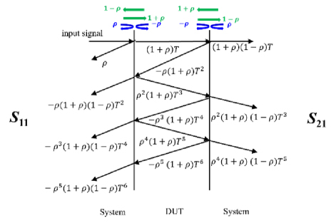
Figure 1: Multiple reflections of a single frequency in the fixture.

After establishing the relationship between the measured S${}_{11}$ and S${}_{21}$, the reflection coefficient $\rho$, and the propagation factor T of the DUT, simultaneous equations can be solved to derive equations (6-8). During this process, it is important to note that there may be two possible solutions for the reflection coefficient $\rho$. However, since the measurement is performed on passive components, where gain is not present, only the solution with $\rho$ less than 1 is valid. This enables the calculation of the reflection coefficient $\rho$ and the propagation factor T of the DUT from the measured S-parameters without prior knowledge of the characteristic impedance of either the DUT or the system:

$\rho$	$=K\pm \sqrt{K^2-1},\left|\rho \right|<1,$	(6)
$K$	$={\displaystyle \frac{S_{11}{}^2-S_{21}{}^2+1}{2S_{11}}},$	(7)
$T$	$={\displaystyle \frac{S_{11}+S_{21}-\rho }{1-\left(S_{11}+S_{21}\right)\rho }}.$	(8)

Once the reflection coefficient $\rho$ and the propagation factor T have been derived from the measured S-parameters, the relationship between the propagation constant $\gamma$${}_D$ of the DUT and the propagation factor T can be obtained, as shown in (9):

$${\gamma }_D=\frac{1}{l}\cdot ln\left(\frac{1}{T}\right).$$

(9)

However, in the calculation process, since S-parameters not only include the magnitude of the voltage wave propagation ratio but also contain important phase information, they are typically represented in complex form. This implies that, during calculations, the reflection coefficient $\rho$, the propagation factor T, and the propagation constant $\gamma$${}_D$of the DUT may exhibit phase ambiguity as a function of frequency. This occurs because the same imaginary value may correspond to different phase angles, requiring careful attention during analysis. To address phase ambiguity, numerical methods such as the unwrap algorithm in MATLAB can be employed to adjust the phase angles. By applying phase continuity correction, the imaginary part of the propagation constant $\gamma$${}_D$ is ln(1/T), as shown in (II.):

$ln\left({\displaystyle \frac{1}{T}}\right)$
$\mathrm{\hspace{1em}\hspace{1em}}=real\left(ln\left({\displaystyle \frac{1}{T}}\right)\right)+j$
$\mathrm{\hspace{1em}\hspace{1em}}*unwrap\left(imag\left(ln\left({\displaystyle \frac{1}{T}}\right)\right)\right).$	(10)

After obtaining the propagation constant $\gamma$${}_D$ of the DUT structure, the next step is to derive the relationship between the wave number k, cutoff wave number k${}_c$, and phase constant $\beta$ of the DUT through Faraday’s Law and Ampere’s Law from Maxwell’s equations in the source-free region. From (11), when the wave number k exceeds the cutoff wave number k${}_c$, the phase constant $\beta$ in the propagation constant $\gamma$${}_D$ of the DUT becomes a real number. Electromagnetic waves can only propagate within the structure when $\beta$ is a real number, which leads to the concept of the cutoff wave number k${}_c$. The cutoff frequency f${}_c$ can be obtained from the cutoff wave number k${}_c$ as shown in (12):

${\gamma }_D^2+k^2$	$=k_c{}^2,$	(11)
$f_c$	$={\displaystyle \frac{k_c}{2\pi \sqrt{\mu ϵ}}}.$	(12)

This study uses coaxial cables to extract the dielectric material properties. During the propagation of electromagnetic waves within a coaxial cable, the electric field, magnetic field, and wave propagation direction are mutually orthogonal. The propagation mode in coaxial cables is the TEM mode. According to the definition of the TEM mode, there are no longitudinal (propagation direction) electromagnetic field components (Ez, Hz) in the guided wave structure.

From (13), the cutoff wave number k${}_c$ for the TEM mode in a coaxial cable is zero. Therefore, by using the propagation constant $\gamma$${}_D$ of the DUT calculated from the measured S-parameters and the wave number k, which is related to the material, as shown in (14), and substituting it into (13), a crucial relationship is obtained as shown in (15), which can then be simplified to (16). In this equation, c is the speed of light in a vacuum (3$\times$10${}^8$ m/sec), which is inversely proportional to the square root of the vacuum permittivity ($ϵ$${}_0$${}_{}$) and vacuum permeability ($\mu$${}_0$), as described in (17). Here, $\omega$ represents the angular frequency, and f represents the frequency:

$k=\omega \sqrt{\mu ϵ},$	(13)
${\gamma }_D^2+k^2=0,$	(14)
${({\gamma }_D)}^2+{(\omega \sqrt{\mu ϵ})}^2=0,$	(15)
${\gamma }_D=j\sqrt{{\displaystyle \frac{{\omega }^2{\mu }_r{ϵ}_r}{c^2}}}=j2\pi \sqrt{{\displaystyle \frac{f^2{\mu }_r{ϵ}_r}{c^2}}},$	(16)
$c={\displaystyle \frac{1}{\sqrt{{ϵ}_0{\mu }_0}}}.$	(17)

The intrinsic impedance $\eta$ of a wave in the dielectric material of the DUT, also known as the wave impedance, is defined in (18). According to the definition of wave impedance, it is proportional to $\mu$/$\gamma$. Assuming that the wave impedance of the system is $\eta$${}_1$ and the wave impedance of the dielectric material in the DUT is $\eta$${}_D$, we can proceed to calculate the reflection coefficient $\rho$ between the system and the DUT using the S-parameters through equation (6). The reflection coefficient $\rho$ is related to the wave impedance $\eta$${}_1$ of the system and the wave impedance $\eta$${}_D$${}_{}$ of the DUT’s dielectric material, as shown in (19):

$\eta$	$={\displaystyle \frac{j\omega \mu }{\gamma }}\propto {\displaystyle \frac{\mu }{\gamma }},$	(18)
$\rho$	$={\displaystyle \frac{{\eta }_2-{\eta }_1}{{\eta }_2+{\eta }_1}}.$	(19)

Assuming that the wave impedance in the system is equal to the wave impedance in a vacuum, i.e., $\eta$${}_1$=$\eta$${}_{\mathrm{0}}$=377 ohm, we substitute the relationship from (18) into (19) and rewrite it as (20). Simplifying further, we obtain (21).

Using equation (21), we can then calculate the relative permeability $\mu$${}_r$(f) of the DUT, as shown in (22). By expressing the propagation constant in a vacuum $\gamma$${}_0$ using equation (16) and calculating the propagation constant $\gamma$${}_D$ of the DUT from equation (9), we can compute $\mu$${}_r$(f), as described in (23):

$\rho$	$={\displaystyle \frac{\frac{{\mu }_2}{{\gamma }_D}-\frac{{\mu }_0}{{\gamma }_0}}{\frac{{\mu }_2}{{\gamma }_D}+\frac{{\mu }_0}{{\gamma }_0}}},$	(20)
$\rho$	$={\displaystyle \frac{\frac{{\gamma }_0}{{\gamma }_D}\cdot {\mu }_r-1}{\frac{{\gamma }_0}{{\gamma }_D}\cdot {\mu }_r+1}},$	(21)
${\mu }_r$	$=({\displaystyle \frac{1+\rho }{1-\rho }}){\displaystyle \frac{{\gamma }_D}{{\gamma }_0}},$	(22)
${\mu }_r$	$=\left({\displaystyle \frac{1+\rho }{1-\rho }}\right){\displaystyle \frac{{\gamma }_D}{j2\pi \sqrt{\frac{f^2}{c^2}}}}.$	(23)

After obtaining the relative permeability $\mu$${}_r$(f) of the DUT, it can be substituted into equation (15) to calculate the relative permittivity $\epsilon$${}_r$(f), as shown in (24). The resulting expression can be simplified as (25). Permittivity $\epsilon$ is a physical property that describes the material’s response to polarization under the influence of an electric field. The real part of $\epsilon$ represents the dielectric’s ability to refract electromagnetic waves, which can be used to calculate how the direction of electromagnetic waves changes as they move from one medium to another. The imaginary part, on the other hand, represents the energy loss within the dielectric, which is caused by the generation of heat from the oscillation of polarized dipoles in the material. Due to energy conservation, the imaginary part of $\epsilon$ must be negative, as described in (26):

${({\gamma }_D)}^2+{(\omega \sqrt{{\mu }_r{\epsilon }_r{\mu }_0{ϵ}_0})}^2=0,$	(24)
${\epsilon }_r=-{\displaystyle \frac{c^2}{{\mu }_r}}\cdot {\left({\displaystyle \frac{{\gamma }_D}{\omega }}\right)}^2,$	(25)
$ϵ={ϵ}^{{}^{\prime }}-j{ϵ}^{{}^{\prime \prime }}={ϵ}^{{}^{\prime }}\left(1-jtan\delta \right).$	(26)

In the calculation process using the Transmission Line Method, the loss term includes both dielectric loss and conductor loss from the coaxial cable, resulting in equation (27). From this, the loss tangent tan$\delta$ of the DUT’s dielectric material (including the metal) can be derived, as shown in (28).

However, it is important to note that, if the dielectric material has very low dielectric loss, the loss tangent value tan$\delta$ calculated from equation (29) may be dominated by the metal losses, preventing an accurate determination of the dielectric material’s tan$\delta$:

$$\nabla \times \overrightarrow{H}=j\omega ϵ\overrightarrow{E}+\overrightarrow{J},$$

(27)

where

$\overrightarrow{J}$	$=\sigma \overrightarrow{E},$
$\nabla \times \overrightarrow{H}$	$=j\omega ϵ\overrightarrow{E}+\sigma \overrightarrow{E}=j\omega {ϵ}^{{}^{\prime }}\overrightarrow{E}+(\omega {ϵ}^{{}^{\prime \prime }}+\sigma )\overrightarrow{E},$	(28)

$$tan\delta =\frac{\omega {ϵ}^{{}^{\prime \prime }}+\sigma }{\omega {ϵ}^{{}^{\prime }}}.$$

(29)

III. EXTRACT INSULATOR PARAMETERS FROM MEASUREMENT

A. Equation formatting

This study prepared three different lengths of coaxial cable samples, with lengths of 15 cm, 30 cm, and 50 cm, and quantities of 10, 10, and 5, respectively, as shown in Fig. 2. According to the manufacturer’s data, the dielectric constant ($\epsilon$${}_r$) of the insulation in the coaxial cables is 2.04$\pm$1% at 1 GHz, and the loss tangent (tan$\delta$) ranges from 0.0002 to 0.0004.

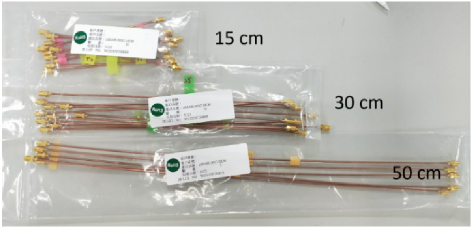
Figure 2: Coaxial cables used for measurement.

Aside from manufacturing tolerances, the three test samples are identical in structure, differing only in length, see Fig. 3. Therefore, two coaxial cables of different lengths were selected for the experiment. The shorter cable was used as the calibration object, while the longer one was used as the error model. The 2X-Thru de-embedding technique was employed to remove the effects of the 3.5 mm SMA connectors, preserving the characteristics of the coaxial cable in between. As a result, the extracted material parameters are free from the influence of the SMA connectors, as illustrated in Fig. 4.

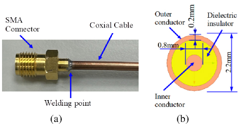
Figure 3: (a) Hand-soldered coaxial cable to SMA connector. (b) Cross-section of the coaxial cable.

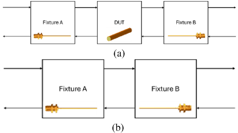
Figure 4: 2X-Thru de-embedded technique. (a) Error model. (b) Thru line.

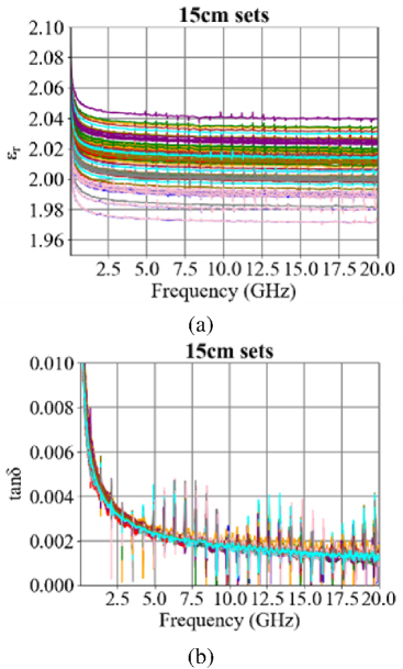
Figure 5: Insulator parameters of the 15 cm coaxial cable are by calculation (a) $\epsilon$${}_r$ and (b) tan$\delta$.

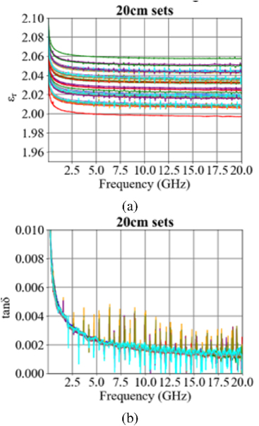
Figure 6: Insulator parameters of the 20 cm coaxial cable are by calculation (a) $\epsilon$${}_r$ and (b) tan$\delta$.

In this experiment, we used two sets of coaxial cables, each comprising ten cables of 15 cm and 30 cm in length, respectively. The S-parameters of each cable were measured using a VNA. Subsequently, a 2X-Thru de-embedding process was applied. The objective was to obtain the parameters of the DUT, which in this case is a 15 cm cable. The error model was based on the measurement of the 30 cm coaxial cable, while the thru line measurement was based on the 15 cm cable. After applying the de-embedding process, we derived 100 sets of S-parameters for the DUT, where the middle 15 cm represents the difference between the 30 cm and 15 cm cables. Using these S-parameters, we calculated 100 sets of $\epsilon$${}_r$ and tan$\delta$, as shown in Fig. 5.

It is important to note that several frequency points exhibited spark-like anomalies. Typically, these issues can be mitigated through more advanced correction methods. The characteristics of the insulator obtained in this study are presented as a range of values.

Next, we selected ten coaxial cables, each 30 cm in length, and five coaxial cables, each 50 cm in length. After measuring the S-parameters of each cable using a VNA, we applied the 2X-Thru de-embedding process. The objective was to obtain the parameters of a 20 cm coaxial cable, which represents the difference between the lengths of the 50 cm and 30 cm cables. The error model was based on measurements of the 50 cm coaxial cable, while the thru line measurement was based on the 30 cm cable. After the de-embedding process, we obtained 50 sets of S-parameters for DUT. From these, we calculated 50 sets, as shown in Fig. 6.

Notably, we observed a reduction in the spike, indicating that the issues associated with the 2X-Thru de-embedding process were mitigated to some extent. As in the previous experiment, the characteristics of the insulator were determined as a range of values.

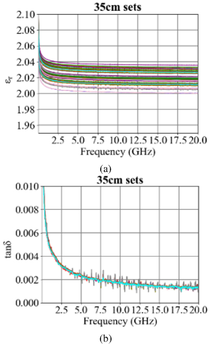
Figure 7: Insulator parameters of the 35 cm coaxial cable are by calculation (a) $\epsilon$${}_r$ and (b) tan$\delta$.

In the third set of experiments, we selected ten coaxial cables, each 15 cm in length, and five coaxial cables, each 50 cm in length. The S-parameters of these cables were measured to obtain the parameters of a 35 cm coaxial cable, representing the difference between the 50 cm and 15 cm cables. The error model was based on measurements of the 50 cm coaxial cable, while the thru line measurement was taken from the 15 cm cable. From these measurements, we calculated 50 sets, as shown in Fig. 7.

We observed a further reduction in the spikes, indicating continued improvement in the issues associated with the de-embedding process. As before, the characteristics of the insulator were presented as a range of values, and this range became more concentrated in this experiment.

Based on the results of the three experiments, we observed a decrease in the anomalous peaks in the extracted material parameters as the length of the DUT increased. This may be due to the fact that, when the DUT is smaller, the discrepancies between the calibration objects and the actual fixtures, as well as manufacturing errors of the DUT itself, have a more pronounced effect. However, as the length of the DUT increases, these non-ideal effects are likely averaged out, leading to more stable extracted material parameters. In the next section, we will use simulations to confirm thishypothesis.

Another issue is the standard deviation of the range of values observed. This variability could stem from differences in the cables, including length, diameter of the conductor and insulator, circularity, surface roughness of the copper conductor, and the degree of foaming in the dielectric layer. When extreme variations exist between cables, the range of values after de-embedding will differ. However, as the DUT length increases, these differences tend to be diluted, resulting in a narrower range of values. To investigate this further, we conducted three additional experiments.

In the first experiment, we used a 15 cm thru line as the calibration object to perform 2X-Thru de-embedding on the 30 cm error model for all cables. The results, shown in Fig. 8, indicate a reduction in the range ofvalues.

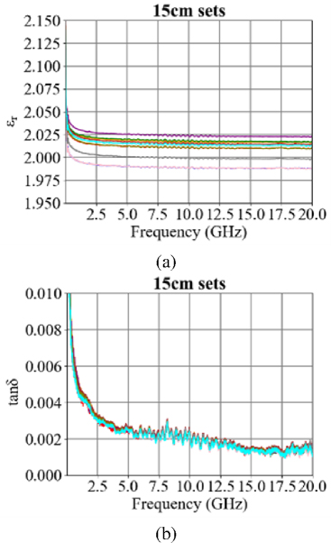
Figure 8: Insulator parameters of the 30 cm by 10sets and 15 cm by 1set (a) $\epsilon$${}_r$ and (b) tan$\delta$.

In the second experiment, we reversed the setup, using ten 15 cm cables as the calibration objects to perform 2X-Thru de-embedding on a single 50 cm error model. The results, shown in Fig. 9, demonstrate an even more concentrated narrowing of the range.

However, we observed that the results of these experiments were unable to yield precise values. Instead, they provide only an estimate of the general range for a batch of produced cables.

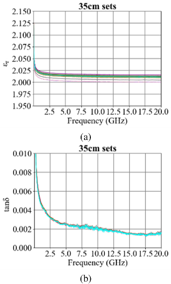
Figure 9: Insulator parameters of the 50 cm by 1set and 15cm by 10sets (a) $\epsilon$${}_r$ and (b) tan$\delta$.

IV. DE-EMBEDDING THEORY

A. Time domain gating

In the standard 2X-Thru calibration method [29], a fixture is connected to create a through line calibration object, which is then used to remove fixture effects from the error model. However, differences between the calibration fixture and the actual fixtures attached to the DUT, or variations in the connections during assembly or measurement, can introduce discrepancies. These differences can be observed through the time-domain response of the fixture in the calibration object and the error model, as shown in Fig. 10.

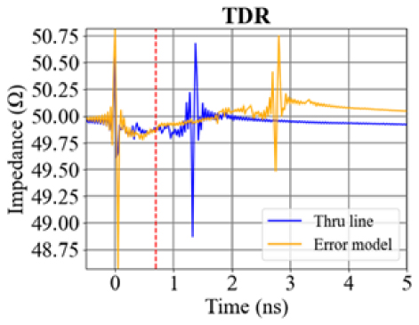
Figure 10: TDR variations in connectors and welding points.

B. De-embedding method

The improved 2X-Thru de-embedding method proposed in this study begins with the same initial steps as the conventional process. However, it assumes excellent impedance matching between the DUT and the fixtures, minimizing reflection at their interface. This assumption aligns with the concept of the Line in TRL calibration [30], where the DUT’s propagation characteristics are represented by e${}^{\mathrm{-}\gamma \mathit{}l}$. In this study, a fixture containing a segment of coaxial cable was selected as the Thru calibration structure to meet these requirements.

In this study, the primary difference between the error model and the calibration object is the presence or absence of the DUT. Assuming that the impedance between the DUT and the fixture is nearly matched, the propagation constant of the DUT, denoted as $\gamma$${}_{ini}$, can be preliminarily estimated using the S-parameters of the error model (|S${}_{T\mathit{}o\mathit{}t\mathit{}a\mathit{}l}$|) and the thru calibration object (|S${}_{T\mathit{}h\mathit{}r\mathit{}u}$|). When the magnitude of S${}_{21}$ of the DUT is high (indicating minimal transmission loss), its value can be expressed by (30). Through (30), the attenuation constant $\alpha$${}_{ini}$ of the DUT can be estimated. Here, $\mathrm{\Delta }$l represents the physical length of the DUT in meters. Next, the phase angles of the transmission coefficients from both the error model and the calibration object are unwrapped to determine the difference in electrical length. This difference corresponds to the electrical length ${\theta }_D$ of the DUT. Consequently, the phase constant ${\beta }_{ini}$ of the DUT can be estimated using (31):

${\alpha }_{ini}$	$={\displaystyle \frac{ln(\mathrm{mag}\left(S_{21,Thru}\right))-ln(\mathrm{mag}\left(S_{21,Total}\right))}{\lambda l}},$	(30)
${\beta }_{ini}$	$={\displaystyle \frac{Phase\left(S_{21,Total}\right)-Phase\left(S_{21,Thru}\right)}{\lambda l}}.$	(31)

By combining (30) and (31), the propagation constant $\gamma$${}_{ini}$ of the DUT can be estimated. Subsequently, by analyzing the signal flow in the error model, equations (32-35) can be derived. In this context, the DUT is assumed to be an ideal transmission line with a propagation characteristic of e${}^{\mathrm{-}}$${}^{\gamma \mathit{}i\mathit{}n\mathit{}i}$, as shown in Fig. 11.

$S_{11}$	$=S_{11A}+{\displaystyle \frac{S_{11B}\cdot S_{21A}^2\cdot e^{-2{\gamma }_{ini}\mathrm{\Delta }l}}{1-S_{22A}\cdot S_{11B}\cdot e^{-2{\gamma }_{ini}\mathrm{\Delta }l}}},$	(32)
$S_{21}$	$={\displaystyle \frac{S_{21A}\cdot S_{21B}\cdot e^{-{\gamma }_{ini}\mathrm{\Delta }l}}{1-S_{22A}\cdot S_{11B}\cdot e^{-2{\gamma }_{ini}\mathrm{\Delta }l}}},$	(33)
$S_{22}$	$=S_{22B}+{\displaystyle \frac{S_{22A}\cdot S_{12B}^2\cdot e^{-2{\gamma }_{ini}\mathrm{\Delta }l}}{1-S_{11B}\cdot S_{22A}\cdot e^{-2{\gamma }_{ini}\mathrm{\Delta }l}}},$	(34)
$S_{12}$	$={\displaystyle \frac{S_{12B}\cdot S_{12A}\cdot e^{-{\gamma }_{ini}\mathrm{\Delta }l}}{1-S_{11B}\cdot S_{22A}\cdot e^{-2{\gamma }_{ini}\mathrm{\Delta }l}}}\mathit{\hspace{1em}}.$	(35)

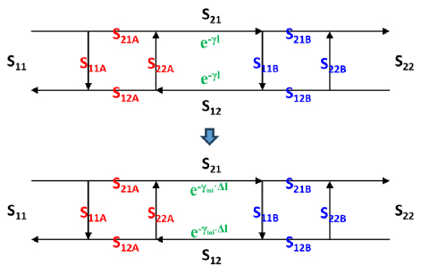
Figure 11: Signal flow graph of error model.

Combine and simplify (32) and (33) into (36), and (34) and (35) into (37):

$S_{11}$	$=S_{11A}+S_{11B}\cdot e^{-{\gamma }_{ini}\mathrm{\Delta }l}\cdot S_{21},$	(36)
$S_{22}$	$=S_{22B}+S_{22A}\cdot e^{-{\gamma }_{ini}\mathrm{\Delta }l}\cdot S_{12}.$	(37)

To determine the reflection coefficients of fixture A and fixture B, we start similarly with |S${}_{\mathrm{11}\mathit{}A}$| from (36) and |S${}_{\mathrm{22}\mathit{}B}$| from (37). However, the process will differ slightly from the existing 2X-Thru calibration procedure.

After obtaining |S${}_{\mathrm{11}\mathit{}A}$| and |S${}_{\mathrm{22}}$${}_B$|, we use (36) and (37) to derive |S${}_{\mathrm{11}\mathit{}B}$| and |S${}_{\mathrm{22}\mathit{}A}$|${}_{}$, as given by (38) and (39). Equations (32) and (34) are employed to determine |S${}_{\mathrm{21}\mathit{}A}$|, |S${}_{\mathrm{12}\mathit{}B}$|, |S${}_{\mathrm{12}\mathit{}A}$|, and |S${}_{\mathrm{21}}$${}_B$| as detailed in (41) and (42):

$S_{11B}$	$={\displaystyle \frac{S_{11}-S_{11\mathrm{A}}}{S_{21}}}\cdot e^{{\gamma }_{ini}\mathrm{\Delta }l},$	(38)
$S_{22A}$	$={\displaystyle \frac{S_{22}-S_{22\mathrm{B}}}{S_{12}}}\cdot e^{{\gamma }_{ini}\mathrm{\Delta }l},$	(39)

$S_{21A}$	$=\sqrt{S_{21}\cdot \left(1-S_{22A}\cdot S_{11B}\cdot e^{-2{\gamma }_{ini}\mathrm{\Delta }l}\right)\cdot e^{{\gamma }_{ini}\mathrm{\Delta }l}}=S_{21B},$	(40)
$S_{12B}$	$=\sqrt{S_{12}\cdot \left(1-S_{11\mathrm{B}}\cdot S_{22\mathrm{A}}\cdot e^{-2{\gamma }_{ini}\mathrm{\Delta }l}\right)\cdot e^{{\gamma }_{ini}\mathrm{\Delta }l}}=S_{12\mathrm{A}}.$	(41)

When the actual S-parameters of the fixtures are obtained, we convert both the fixture S-parameters and the error model S-parameters into T-parameter matrices. By performing the de-embedding calculations, we derive the DUT’s T-parameters, which are then converted back to S-parameters.

V. SIMULATION AND VALIDATION

A. Simulation

In this section, a circuit simulator is used to simulate two-port networks with COAX components to model the S-parameters of the calibration object and error model. The DUT is a 50-ohm, 150-mm COAX component. The simulation accounts for connector transition effects and variations in the coaxial cable’s insulation diameter (Do), reflecting connector characteristics and dis-continuities. Simulation data are presented in Tables 1–3.

Table 1: Cross-section dimensions of DUT

Outer Radius (Do)	Length (L)	Characteristic Impedance (Z${}_{\mathrm{0}}$)	DUT
1.072 mm	150 mm	50.02$\mathrm{\Omega }$	COAX inner diameter (Di) is fixed at 0.32 mm

Table 2: Cross-section dimensions of Calibration Object

	Outer Radius (Do)	Length (L)	Characteristic Impedance (Z${}_{\mathrm{0}}$)
Fixture A	1.062 mm	2 mm	49.63$\mathrm{\Omega }$
	1.078 mm	10 mm	50.25$\mathrm{\Omega }$
	1.065 mm	2 mm	49.75$\mathrm{\Omega }$
	1.072 mm	50 mm	50.02$\mathrm{\Omega }$
Fixture B	1.072 mm	50 mm	50.02$\mathrm{\Omega }$
	1.065 mm	2 mm	49.75$\mathrm{\Omega }$
	1.078 mm	10 mm	50.25$\mathrm{\Omega }$
	1.062 mm	2 mm	50.02$\mathrm{\Omega }$
COAX inner diameter (Di) is fixed at 0.32 mm

Table 3: Cross-section dimensions of Calibration Object-1

	Outer Radius (Do)	Length (L)	Characteristic Impedance (Z${}_{\mathrm{0}}$)
Fixture A	1.059 mm	2 mm	49.51$\mathrm{\Omega }$
	1.066 mm	10 mm	49.78$\mathrm{\Omega }$
	1.074 mm	2 mm	50.10$\mathrm{\Omega }$
	1.072 mm	50 mm	50.02$\mathrm{\Omega }$
Fixture B	1.072 mm	50 mm	50.02$\mathrm{\Omega }$
	1.074 mm	2 mm	50.10$\mathrm{\Omega }$
	1.066 mm	10 mm	49.78$\mathrm{\Omega }$
	1.059 mm	2 mm	49.51$\mathrm{\Omega }$
COAX inner diameter (Di) is fixed at 0.32 mm

This study compares two main aspects. First, it examines the de-embedding results before and after improvements when the calibration fixtures match the DUT fixtures. Second, it analyzes the results using a different calibration object (Calibration Object-1) when the fixtures differ. Both the IEEE P370 standard 2X-Thru de-embedding algorithm and an enhanced Python-based algorithm are employed to process the S-parameters of the DUT.

B. Validation

The S-parameters of the calibration fixtures obtained through different algorithms are compared with the S-parameters of the DUT fixtures (Golden Standard) simulated in a circuit simulator, as illustrated in Fig. 12. The blue line represents the S-parameters obtained using the existing 2X-Thru de-embedding algorithm, while the yellow line indicates those obtained with the improved method proposed in this study. The green line shows the S-parameters from the circuit simulator for a single fixture. The results demonstrate that the improved 2X-Thru de-embedding algorithm yields S-parameters that closely align with both the existing algorithm and the simulated fixture S-parameters, as shown in Fig. 13.

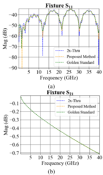
Figure 12: Fixture S-parameter comparison (match) (a) |S${}_{11}$| and (b) |S${}_{21}$.

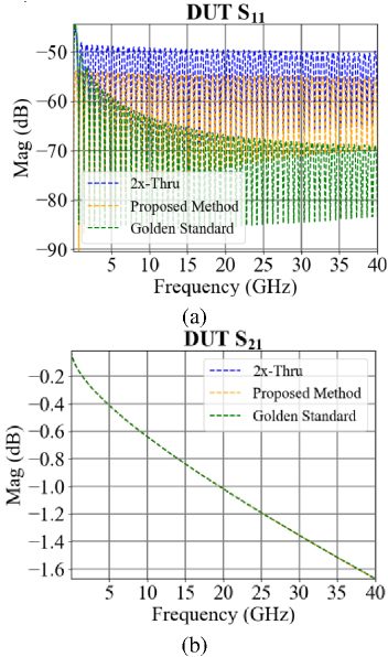
Figure 13: DUT S-parameter comparison (match) (a) |S${}_{11}$| and (b) |S${}_{21}$|.

In practical applications, measurement or fabrication errors can cause slight differences between the calibration fixtures and those used next to the DUT. This study uses Calibration Object-1 to de-embed the error model. Analysis of the time-domain reflection impedance reveals a minor discrepancy between the trace impedance of the left fixture in Calibration Object-1 and that in the error model, as indicated by the impedance before the red dashed line in Fig. 14. The calibration and de-embedding results are shown in Figs. 15 and 16.

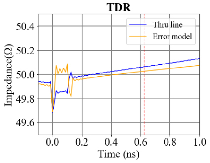
Figure 14: Difference in time domain reflection.

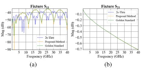
Figure 15: Fixture S-parameter comparison (differ) (a) |S${}_{11}$| and (b) |S${}_{21}$|.

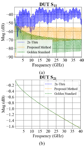
Figure 16: DUT S-parameter comparison (differ) (a) |S${}_{11}$| and (b) |S${}_{21}$|.

VI. MEASUREMENT

Here, we use the Nicolson-Ross-Weir (NRW) method to validate the parameter extraction methods for coaxial cable insulation. Ignoring manufacturing errors, the samples differ only in length. Both the existing 2X-Thru de-embedding algorithm and the improved version were used to remove the 3.5 mm connector effects and isolate the coaxial cable properties.

We analyzed the extracted $\epsilon$${}_r$ and tan$\delta$ across different combinations. We identified the maximum and minimum values at each frequency using various de-embedding methods, as illustrated in Fig. 17. Observation shows that the improved 2X-Thru de-embedding algorithm effectively reduces numerical errors caused by differences between calibration objects and actual fixtures. Our method effectively reduces the spikes caused by after de-embedding at specific frequencies, enhancing the precision of the extracted values. However, due to manufacturing tolerances, the extracted $\epsilon$${}_r$ and tan$\delta$ result in a range of values rather than a single point.

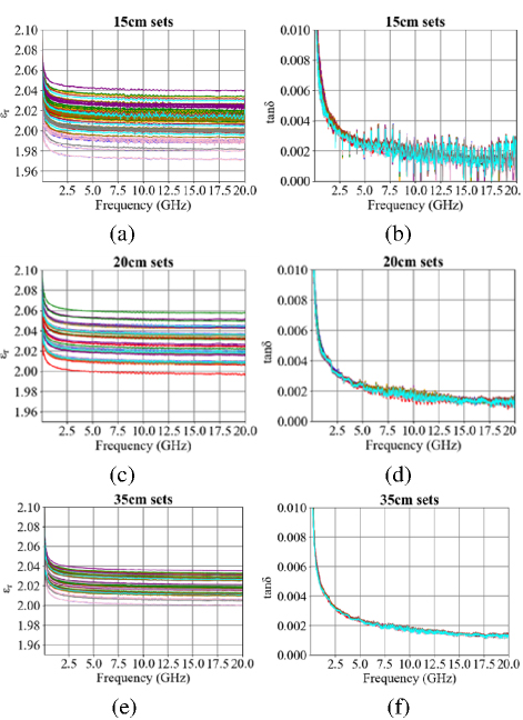
Figure 17: Extracted values of cable insulators by the improved 2X-Thru method (a) 15 cm, $\epsilon$${}_r$ (b) 15 cm, tan$\delta$ (c) 20 cm, $\epsilon$${}_r$(d) 20 cm, tan$\delta$ (e) 35 cm, $\epsilon$${}_r$ (f) 35 cm, tan$\delta$.

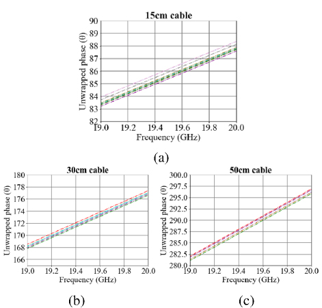
Figure 18: Original phase |S${}_{21}$| of coaxial cable (a) 15 cm, (b) 30 cm, and (c) 50 cm.

Table 4: Comparison among the classical methods

	[16]	[19]	[31]	This work
Method	Open-ended Coaxial	Free space	Waveguide	Coaxial line
DUT Material	PTFE	Flat plastic	Flat plastic	Cable insulator
Fixture	SMA	Antenna	X-band Waveguide	SMA
Input	S${}_{11}$, S${}_{12}$	S${}_{11}$, S${}_{12}$	S${}_{11}$, S${}_{12}$	S${}_{11}$, S${}_{12}$
Output	$\epsilon$${}_r$	$\epsilon$${}_r$	$\epsilon$${}_r$	$\epsilon$${}_r$, tan $\delta$
Frequency	0-20 GHz	8.2-12 GHz	8.2-12 GHz	0-20 GHz
Range	Broad band	Wide	Wide	Broad band
For production inspection	No	No	No	Yes

We also observed that, under the same length configuration, slight variations are present in the extracted results regardless of whether the same error model is de-embedded using different calibration artifacts or the same calibration artifact is used to de-embed different error models. These variations can be attributed to measurement differences. The coaxial cable lengths and labels provided by manufacturers typically have a tolerance of approximately $\pm$3 mm, as verified through the measured phase of |S${}_{21}$|, as shown in Fig. 18. By examining the |S${}_{21}$| original phase of the coaxial cables, it is evident that the electrical length of each sample labeled with the same length exhibits minor differences. Since the electrical length is related to the phase constant and physical dimensions, as indicated in (42), these length tolerances result in discrepancies in the extracted material parameters. Finally, the advantages summarized in Table 4 are validated:

$$\theta =\beta l.$$

(42)

VII. CONCLUSION

This study proposes a method for extracting the relative permittivity of cables that more closely reflects their actual properties. Compared to the traditional open-end coaxial line structure, we adopt an extruding machine to injection-mold the insulator, resulting in a device with virtually no air gaps. During the measurement process, manufacturing tolerances in the production of the sample and the actual length of the coaxial cables introduce variability. Additionally, inconsistencies in the size of solder joints between the coaxial cable and SMA connectors further contribute to de-embedding errors. To address these challenges, we present an improved version of the 2X-Thru de-embedding method and conduct comparative evaluations. The proposed method significantly reduces numerical errors, offering a more reliable approach for accurately extracting material parameters in practical applications. Results indicate that as the measured cable length increases, the extracted values converge within a narrower range, and the occurrence of spikes is reduced. This improvement may be attributed to the greater impact of calibration object discrepancies and cable manufacturing tolerances when the cable size is smaller. However, as the cable length increases, the non-ideal effects become more evenly distributed, resulting in smoother and more stable material parameter extraction.

ACKNOWLEDGMENT

This work was supported by BizLink International Corporation.

REFERENCES

[1] IEEE Standard for Ethernet Amendment 2: Physical Layer Specifications and Management Parameters for 100 GB/s Operation Over Backplanes and Copper Cables, IEEE Std 802.3bj-2014 (Amendment to IEEE Std 802.3-2012 as amended by IEEE Std 802.3bk-2013), pp. 1-368, 3 Sep. 2014.

[2] E. Mayevskiy and H. James, “Limitations of the intra-pair skew measurements in gigabit range interconnects,” DesignCon, 2016.

[3] Z. Chen, M. Prasad, D. O’Connor, P. Bond, and A. Muszynski, “Differential TwinAx cable modeling by measured 4-port S-parameters,” in Proc. IEEE 14th Topical Meeting Elect. Perform. Electron. Package, pp. 87-90, 2005.

[4] Y. Shlepnev and C. Nwachukwu, “Modelling jitter induced by fibre weave effect in PCB dielectrics,” Proc. IEEE Int. Symp. Electromagnet. Compat., pp. 803-808, 2014.

[5] E. J. Denlinger, “Frequency dependence of a coupled pair of microstrip lines (correspondence),” IEEE Trans. Microwave Theory Tech., vol. 18, no. 10, pp. 731-733, Oct. 1970.

[6] Y. Liu, S. Bai, C. Li, V. S. De Moura, B. Chen, and S. Venkataraman, “Inhomogeneous dielectric induced skew modeling of TwinAx cables,” IEEE Transactions on Signal and Power Integrity, vol. 2, pp. 94-102, 2023.

[7] A. Talebzadeh, K. Koo, P. K. Vuppunutala, J. Nadolny, A. Li, and Q. Liu “SI and EMI performance comparison of standard QSFP and flyover QSFP connectors for 56+ GBps applications,” Proc. IEEE Int. Symp. Electromagnet. Compat. Signal/Power Integrity, pp. 776-781, 2017.

[8] W. H. Tsai, D. B. Lin, T. F. Tseng, and C. H. Ho, “Analysis of electrical characteristics of TwinAx cable with asymmetric structures,” in 2024 IEEE Joint International Symposium on Electromagnetic Compatibility, Signal & Power Integrity: EMC Japan / Asia-Pacific International Symposium on Electro-magnetic Compatibility (EMC Japan /APEMC Okinawa), Ginowan, Okinawa, Japan, pp. 342-345, 2024.

[9] R. Joshi, S. K. Podilchak, C. Constantinides, and B. Low, “Flexible textile-based coaxial transmission lines for wearable applications,” IEEE Journal of Microwaves, vol. 3, no. 2, pp. 665-675, Apr.2023.

[10] A. Lago, C. M. Penalver, J. Marcos, J. D. Gandoy, A. A. N. Melendez, and O. Lopez, “Electrical design automation of a twisted pair to optimize the manufacturing process,” IEEE Trans. on Components, Packaging and Manufacturing Technology, vol. 1, no. 8, pp. 1269-1281, Aug. 2011.

[11] Telephone cable. Test methods, Moscow: Standards Publishing House, GOST (State Standard) 27893-88, 1989.

[12] S. Yasufuku, T. Umemura, and Y. Ishioka, “Phenyl methyl silicone fluid and its application to high-voltage stationary apparatus,” IEEE Transactions on Electrical Insulation, vol. EI-12, no. 6, pp. 402-410, Dec. 1977.

[13] R. M. Hakim, R. G. Olivier, and H. St-Onge, “The dielectric properties of silicone fluids,” IEEE Transactions on Electrical Insulation, vol. EI-12, no. 5, pp. 360-370, Oct. 1977.

[14] Cables, wires and cords. Methods of voltage testing, Moscow: Standards Publishing House, GOST (State Standard) 2990-72, 1986.

[15] A. Goldshtein, G. Vavilova, and S. Mazikov, “Capacitance control on the wire production line,” IME&T, 2016.

[16] I. Dilman, M. N. Akinci, T. Yilmaz, M. Çayören, and I. Akduman, “A method to measure complex dielectric permittivity with open-ended coaxial probes,” IEEE Transactions on Instrumentation and Measurement, vol. 71, pp. 1-7, 2022.

[17] D. Popovic, L. McCartney, C. Beasley, M. Lazebnik, M. Okoniewski, and S. C. Hagness, “Precision open-ended coaxial probes for in vivo and ex vivo dielectric spectroscopy of biological tissues at microwave frequencies,” IEEE Transactions on Microwave Theory and Techniques, vol. 53, no. 5, pp. 1713-1722, May 2005.

[18] M. J. Da Silva, E. Schleicher, and U. Hampel, “A novel needle probe based on high-speed complex permittivity measurements for investigation of dynamic fluid flows,” IEEE Trans. on Instrumentation and Measurement, vol. 56, no. 4, pp. 1249-1256, Aug. 2007.

[19] H. Shwaykani, J. Costantine, A. El-Hajj, and M. Al-Husseini, “Monostatic free-space method for relative permittivity determination using horn antenna near-field measurements,” IEEE Antennas and Wireless Propagation Letters, vol. 23, no. 4, pp. 1336-1340, Apr. 2024.

[20] B. Moon and J. Oh, “FSS-enhanced quasi-optical dielectric measurement method for liquid crystals in sub-THz band,” IEEE Antennas and Wireless Propagation Letters, vol. 22, no. 12, pp. 3062-3066, Dec. 2023.

[21] L. S. Rocha, C. C. Junqueira, E. Gambin, A. N. Vicente, A. E. Culhaoglu, and E. Kemptner, “A free space measurement approach for dielectric material characterization,” in 2013 SBMO/IEEE MTT-S International Microwave & Optoelectronics Conference (IMOC), Rio de Janeiro, Brazil,2013.

[22] J.-M. Heinola, P. Silventoinen, K. Latti, M. Kettunen, and J.-P. Strom, “Determination of dielectric constant and dissipation factor of a printed circuit board material using a microstrip ring resonator structure,” in 15th International Conference on Microwaves, Radar and Wireless Communications (IEEE Cat. No.04EX824), Warsaw, Poland, vol. 1, pp. 202-205, 2004.

[23] G. Galindo-Romera, F. Javier Herraiz-Martínez, M. Gil, J. J. Martínez-Martínez, and D. Segovia-Vargas, “Submersible printed split-ring resonator-based sensor for thin-film detection and permittivity characterization,” IEEE Sensors Journal, vol. 16, no. 10, pp. 3587-3596, May 2016.

[24] H. Shwaykani, A. El-Hajj, J. Costantine, F. A. Asadallah, and M. Al-Husseini, “Dielectric spectroscopy for planar materials using guided and unguided electromagnetic waves,” in 2018 IEEE Middle East and North Africa Communications Conference (MENACOMM), Jounieh, Lebanon, pp. 1-5, 2018.

[25] H. B. Wang and Y. J. Cheng, “Broadband printed-circuit-board characterization using multimode substrate-integrated-waveguide resonator,” IEEE Transactions on Microwave Theory and Techniques, vol. 65, no. 6, pp. 2145-2152, June 2017.

[26] W. B. Weir, “Automatic measurement of complex dielectric constant and permeability at microwave frequencies,” Proceedings of the IEEE, vol. 62, no. 1, pp. 33-36, Jan. 1974.

[27] B. Chen, X. Ye, B. Samaras, and J. Fan, “A novel de-embedding method suitable for transmission-line measurement,” in 2015 IEEE APEMC, Taipei, Taiwan, 2015.

[28] Y.-C. Luo, Y.-H. Chen, C.-Y. Zhuang, J.-H. Lu, and D.-B. Lin, “The bandwidth limitation of de-embedding technique for microstrip line measurement,” in 2023 VTS Asia Pacific Wireless Communications Symposium (APWCS), Tainan City, Taiwan, 2023.

[29] IEEE Standard for Electrical Characterization of Printed Circuit Board and Related Interconnects at Frequencies up to 50 GHz, IEEE Std 370-2020, pp. 1-147, 8 Jan. 2021

[30] B. Hofmann and S. Kolb, “A multi standard method of network analyzer self-calibration-generalization of multiline TRL,” IEEE Transactions on Microwave Theory and Techniques, vol. 66, no. 1, pp. 245-254, Jan. 2018.

[31] C. Yang and H. Huang, “Extraction of stable complex permittivity and permeability of low-loss materials from transmission/reflection measurements,” IEEE Transactions on Instrumentation and Measurement, vol. 70, pp. 1-8, 2021.

BIOGRAPHIES

Wei-Hsiu Tsai received the B.S. degree in Mathematics from the Fu Jen Catholic University, New Taipei, Taiwan, in 1999, and the M.B.A. degree in industrial management from the National Taiwan University of Science and Technology (Taiwan Tech), Taipei, Taiwan, in 2019. He is pursuing a Ph.D. degree in the Department of Electronic and Computer Engineering, National Taiwan University of Science and Technology (Taiwan Tech) under the supervision of Professor Ding-Bing Lin. He is currently an Engineer with BizLink International Corp., New Taipei, Taiwan. His research interests include high-speed transmission techniques and high-frequency measurement techniques.

Ding-Bing Lin (S’89-M’93-SM’14) received the M.S. and Ph.D. degrees in electrical engineering from National Taiwan University, Taipei, Taiwan, in 1989 and 1993, respectively. From August 1993 to July 2016, he was in the faculty of the Electronic Engineering Department, National Taipei University of Technology, Taipei, Taiwan, where he was an Associate Professor, a Professor and a Distinguished Professor in 1993, 2005 and 2014, respectively. Since August 2016, he had been with National Taiwan University of Science and Technology, Taipei, Taiwan, where he is currently a Professor in the Electronic and Computer Engineering Department. His research interests include wireless communication, antennas, high-speed digital transmission and microwave engineering. From 2015 to 2018, he served as the Taipei Chapter Chair, IEEE EMC society. Since 2022, he serves as the Taipei Chapter Chair, IEEE AP society. He also serves as Associate Editor of IEEE Transactions of Electromagnetic Compatibility since 2019 and Editorial Board member of the International Journal of Antennas and Propagation since 2014. He has published more than 250 papers in international journals and conferences. Lin was the recipient of the Annual Research Outstanding Award of the College of Electrical Engineering and Computer Science in 2004, 2006 and 2008. Subsequently, the College of Electrical Engineering and Computer Science awarded him the College Research Outstanding Award to highlight his research achievements. He was also the recipient of the Taipei Tech Annual Outstanding Research Award in 2008. Lin was the recipient of the Annual Research Outstanding Award of the National Taiwan University of Science and Technology in 2024.

Po-Jui Lu received the B.S. degree from Department of Electrical Engineering, National University of Kaohsiung, Kaohsiung, Taiwan, in 2022, and the M.S. degree in Electronic and Computer Engineering from the National Taiwan University of Science and Technology, Taipei, Taiwan, in 2024. His research interests includes high-frequency measurement techniques, signal integrity and power integrity.

Tzu-Fang Tseng received the B.S. degree in electrical engineering from National Taiwan University, Taipei, Taiwan, in 2009, and the Ph.D. degree in photonics and opto-electronics from National Taiwan University, Taipei, Taiwan, in 2015. She started working in industry in 2015. Her research interests include MMW signal transmission, signal integrity in high-speed cables and connectors, and optical planar lightwave circuit design and applications.

ACES JOURNAL, Vol. 40, No. 6, 550–563
doi: 10.13052/2024.ACES.J.400608
© 2025 River Publishers