Calculation of Bending Effects on the Lumped Inductance for Cables Using the Line Current Model

Xiao Chen¹, Haicheng Yin², Gang Zhang¹, Francesco de Paulis³, and Xin He⁴

¹School of Electrical Engineering and Automation Harbin Institute of Technology, Harbin, HL 150001, China
chenxiaoshawn@foxmail.com, zhang_hit@hit.edu.cn

²No. 23 Research Institute of CETC Shanghai, SH 201900, China
gloriachild@126.com

³UAq Electromagnetic Compatibility Lab University of L’Aquila, L’Aquila, Abruzzi 67100, Italy
francesco.depaulis@univaq.it

⁴Department of Mechanical Engineering and Automation Harbin Institute of Technology, Shenzhen, GZ 518000, China
21B953013@stu.hit.edu.cn

Submitted On: April 21, 2025; Accepted On: December 12, 2025

ABSTRACT

This paper presents a semi-analytical method to calculate the bending effects on cable inductance at low frequencies using the line current model (LCM). To deal with the divergent items of the self-inductance obtained by the LCM, some cautious treatments are adopted to counteract the divergent terms between the straightened LCM and bent LCM, leading to a semi-analytical formula for the inductance deviation of the parallel-pair cable. The LCM is then applied to the coaxial cable in collaboration with the decomposition of the conductors, to take into account the mutual inductance among the portions of each conductor. The results of the proposed semi-analytical method are compared with those obtained by the finite element method (FEM), which validates the accuracy of the method. Furthermore, the dependence of the inductance deviation on cable parameters is illuminated for reference of realistic inductance determination.

Keywords: Cable inductance, line current model, partial inductance, semi-analytical method.

1 INTRODUCTION

The measurement method for coaxial cable inductance at low frequencies has been defined in a standard [1], where a cable sample longer than 10 m is required to be straightened for the accurate inductance measurement result. However, there is generally no adequate space to place a straightened cable with a length over 10 m in a laboratory, impairing the practical applicability of the standard. Therefore, if the deviations of cable inductance between the straight layout and bending layouts are determined, the inductance in a straight layout may be obtained through modification of that measured in a bending case where modest space is expected.

Despite closed-form formulas for the inductance in some ideal cases [2, 3, 4], the calculation of inductance for conductors characterized by complicated cross-sections and arbitrary shapes relies on numerical methods [5, 6]. Moreover, specific methods with the simplification of conductor shapes, such as the surface current model (SCM) and line current model (LCM), can be used to obtain analytical or analytical-numerical results for some less complicated cases like coils. SCM is used to handle the circular cross-section for an arbitrary-shaped coil, to reduce the complexity of the subsequent finite element method (FEM) for the calculation of the inductance [7]. The mutual inductance of circular and elliptic coils is analytically deduced in the LCM, resulting in expressions involving Bessel and Struve functions [8]. There has been yet no research that exploits the LCM for the calculation of the selfinductance, because the corresponding integral does not converge.

In this paper, the LCM is adopted to deduce the cable inductance, where both the self and mutual inductances of the conductors are necessary. The divergent self-inductance integral is specially treated such that the deviation of the cable inductance between the straightened and bent layouts can be calculated. The LCM is directly applied to the parallel-pair cable, generating an accurate and efficient semi-analytical formula for the inductance deviation, which is then utilized to acquire the inductance deviation of the coaxial cable precisely by decomposing into several parallel-pairs.

2 BASIC FORMULATION OF CABLE INDUCTANCE

When the lumped inductance of a cable is measured at low frequencies below 10 kHz, the cable is assumed to be configured as Fig. 1, where one end of the cable is connected to an LCR meter and the other end is shorted. The lumped impedance of the cable can be depicted as shown in Fig. 2, where $R_1$ and $R_2$ are the resistances of the two conductors, $L_1$ and $L_2$ are the partial self-inductances of the conductors, and $M_{12}$ is the mutual inductance between the conductors. The impedance of the shorting wire and the capacitance between the conductors of the cable are neglected.

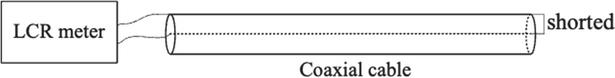
Figure 1 Configuration for inductance measurement of the cable.

The (lumped) inductance $L$ can be expressed as:

$$L=L_1+L_2-2M_{12}.$$

(1)

If each conductor has a uniform cross-section and there is no ambient permeability magnetic material, those partial inductances at low frequencies can be calculated by the quasi-static formula as the following integral [9]:

$$L_{mn}=\frac{{\mu }_0}{4\pi S_m{S}_n}{\int }_{l_m}{\int }_{l_n}{\int }_{A_m}{\int }_{A_n}\frac{{\overrightarrow{t}}_m\cdot {\overrightarrow{t}}_n}{r_{mn}}d{A}_{n}d{A}_{m}d{l}_{n}d{l}_m,$$

(2)

where both $m$ and $n$ belong to $\{1,2\};L_{\mathrm{mn}}$ is the partial inductance, and it is noted that $L_{11}=L_1,L_{22}=L_2$, and $L_{12}=L_{21}=M_{12};{\mu }_0$ is the permeability of vacuum; $S_m$ and $S_n$ are the areas of the conductor cross-sections; $l_m$ and $l_n$ are the one-dimensional integration regions along the axes. $A_m$ and $A_n$ are the two-dimensional integration regions in the cross-sections; ${\overrightarrow{t}}_m$ and ${\overrightarrow{t}}_n$ are the unit tangent vectors of $l_m$ and $l_n$, respectively; $r_{mn}$ is the distance between the integration cells in the two regions.

The six-fold integral in (2) is sophisticated but extremely hard for analytical solution. Hence, it is approximated that the integral kernel keeps constant in the integration cross-sections, which in fact ignores the cross-section shapes and converts the two conductors into LCMs. Then, the simplified integral reads:

$$L_{mn}\approx \frac{{\mu }_0}{4\pi }{\int }_{l_m}{\int }_{l_n}\frac{{\overrightarrow{t}}_m\cdot {\overrightarrow{t}}_n}{r_{mn}}d{l}_{n}d{l}_m.$$

(3)

The following section is to solve (3) for the parallel-pair and coaxial cables at the straightened layout and bent layouts, respectively. Consequently, the deviations of the inductance between different layouts are obtained.

3 DEDUCTION OF INDUCTANCE DEVIATION

3.1 Parallel-pair cable

It is assumed that, for the parallel-pair cable, the conductors have circular cross-sections and both the conductors and the insulation are composed of nonferromagnetic material.

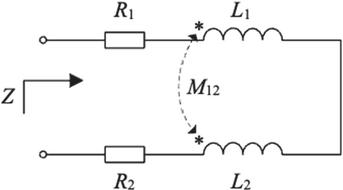
Figure 2 Schematic diagram of the equivalent circuit for the cable under test.

In regard to a straightened parallel-pair cable with length $l$ and conductor distance $d$, the LCM in Fig. 3 can be used to calculate partial inductances:

$$L_{11\mathrm{s}}=L_{22\mathrm{s}}=\frac{{\mu }_0}{4\pi }{\int }_0^l{\int }_0^l\frac{1}{|x_2-x_1|}d{x}_{2}d{x}_1,$$	(4)
$$L_{12\mathrm{s}}=L_{21\mathrm{s}}=\frac{{\mu }_0}{4\pi }{\int }_0^l{\int }_0^l\frac{1}{\sqrt{{(x_2-x_1)}^2+d^2}}d{x}_{2}d{x}_1,$$	(5)

where $L_{mn\mathrm{s}}$ is the partial inductance for the straightened parallel-pair cable.

The inner integral in (4) includes a divergent improper integral that even does not have a finite Cauchy principal value due to the absolute value operator. However, the integral interval can be separated to constitute possible proper integrals:

	${\displaystyle {\int }_0^l}{\displaystyle \frac{\mathrm{d}{x}_2}{\left|x_2-x_1\right|}}$
	$={\displaystyle {\int }_0^{x_1-\delta }}{\displaystyle \frac{\mathrm{d}{x}_2}{x_1-x_2}}+{\displaystyle {\int }_{x_1-\delta }^{x_1+\delta }}{\displaystyle \frac{\mathrm{d}{x}_2}{\left|x_2-x_1\right|}}+{\displaystyle {\int }_{x_1+\delta }^l}{\displaystyle \frac{\mathrm{d}{x}_2}{x_2-x_1}}$
	$=\ln \left({\displaystyle \frac{x_1}{\delta }}\right)+{\displaystyle {\int }_{x_1-\delta }^{x_1+\delta }}{\displaystyle \frac{\mathrm{d}{x}_2}{|x_2-x_1|}}+\ln \left({\displaystyle \frac{l-x_1}{\delta }}\right),$	(6)

where $\delta >0$ is the half length of the divergent interval and independent with $x_1$ or $x_2$.

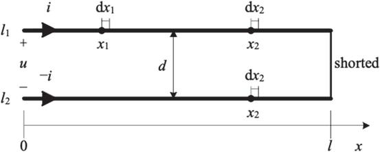
Figure 3 LCM for the straightened parallel-pair cable.

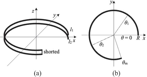
Figure 4 LCM for the bent parallel-pair cable: (a) illustrative diagram and (b) top view.

The divergent second item in (3.1) is caused by the LCM and would converge if the integration were implemented in a two-dimensional or three-dimensional space. By denoting this item as $I_0$ and implementing the outer integration, $L_{11\mathrm{s}}$ can be expressed as:

$$L_{11\mathrm{s}}=\frac{{\mu }_{0}l}{4\pi }(I_0+2\ln l-2\ln \delta -2).$$

(7)

The solution to (5) is trivial:

$L_{12\mathrm{s}}={\displaystyle \frac{{\mu }_{0}l}{2\pi }}\left[l\ln (l+\sqrt{l^2+d^2})+d-\sqrt{l^2+d^2}-l\ln d\right].$

(8)

Then, according to (1), the inductance of a straightened parallel-pair cable is:

$L_{\mathrm{s}}$	$=2L_{11\mathrm{s}}-2L_{12\mathrm{s}}$
	$={\displaystyle \frac{{\mu }_{0}l}{2\pi }}[I_0+2\ln (ld)+{\displaystyle \frac{2\sqrt{l^2+d^2}}{l}}$
	$-2\ln (l+\sqrt{l^2+d^2})-2\ln \delta -{\displaystyle \frac{2d}{l}}-2].$	(9)

To investigate the bending effect on the inductance of a parallel-pair cable, an arc-shaped parallel-pair cable in the LCM is constructed as illustrated in Fig. 4. The cable in the same length $l$ and conductor distance $d$ is bent along the track of an arc of radius $R$ and angle ${\theta }_{\mathrm{m}}\in (0,2\pi )$, thus:

$$R=\frac{l}{{\theta }_{\mathrm{m}}}.$$

(10)

The self and mutual inductances can be calculated by the following integrals:

$L_{11\mathrm{b}}$	$=L_{22\mathrm{b}}={\displaystyle \frac{{\mu }_0{R}_b}{8\pi }}{\displaystyle {\int }_0^{{\theta }_{\mathrm{m}}}}{\displaystyle {\int }_0^{{\theta }_{\mathrm{m}}}}{\displaystyle \frac{\cos ({\theta }_2-{\theta }_1)}{\left|\sin \frac{{\theta }_2-{\theta }_1}{2}\right|}}d{\theta }_{2}d{\theta }_1,$	(11)
$L_{12\mathrm{b}}$	$=L_{21\mathrm{b}}$
	$={\displaystyle \frac{{\mu }_0{R}^2}{4\pi }}{\displaystyle {\int }_0^{{\theta }_{\mathrm{m}}}}{\displaystyle {\int }_0^{{\theta }_{\mathrm{m}}}}{\displaystyle \frac{\cos \left({\theta }_2-{\theta }_1\right)\mathrm{d}{\theta }_2\mathrm{d}{\theta }_1}{\sqrt{2R^2-2R^2\cos \left({\theta }_2-{\theta }_1\right)+d^2}}},$	(12)

where $L_{mn\mathrm{b}}$ is the partial inductance for the bent parallel-pair cable.

The inner integral in (11) can be treated similarly to the straightened case:

$${\int }_0^{{\theta }_{\mathrm{m}}}\frac{\cos \left({\theta }_2-{\theta }_1\right)}{\left|\sin \frac{{\theta }_2-{\theta }_1}{2}\right|}d{\theta }_2=K_1+K_2+K_3$$

(13)

where:

$K_1$	$={\displaystyle {\int }_0^{{\theta }_1-\frac{\delta }{R}}}{\displaystyle \frac{\cos \left({\theta }_2-{\theta }_1\right)}{\sin \frac{{\theta }_1-{\theta }_2}{2}}}d{\theta }_2$
	$=4\cos {\displaystyle \frac{{\theta }_1}{2}}+2\ln \left(\tan {\displaystyle \frac{{\theta }_1}{4}}\right)$
	$-4\cos {\displaystyle \frac{\delta }{2R}}-2\ln \left(\tan {\displaystyle \frac{\delta }{4R}}\right),$	(14)
$K_2$	$={\displaystyle {\int }_{{\theta }_1-\frac{\delta }{R}}^{{\theta }_1+\frac{\delta }{R}}}{\displaystyle \frac{\cos \left({\theta }_2-{\theta }_1\right)}{\left|\sin \frac{{\theta }_2-{\theta }_1}{2}\right|}}d{\theta }_2,$	(15)

and:

$K_3$	$={\displaystyle {\int }_{{\theta }_1+\frac{\delta }{R}}^{{\theta }_{\mathrm{m}}}}{\displaystyle \frac{\cos \left({\theta }_2-{\theta }_1\right)}{\sin \frac{{\theta }_2-{\theta }_1}{2}}}d{\theta }_2$
	$=4\cos {\displaystyle \frac{{\theta }_{\mathrm{m}}-{\theta }_1}{2}}+2\ln \left(\tan {\displaystyle \frac{{\theta }_{\mathrm{m}}-{\theta }_1}{4}}\right)$
	$-4\cos {\displaystyle \frac{\delta }{2R}}-2\ln \left(\tan {\displaystyle \frac{\delta }{4R}}\right).$	(16)

If $\delta$ is small enough, $\cos ({\theta }_2-{\theta }_1)\approx 1$ and $\sin \frac{{\theta }_1-{\theta }_2}{2}\approx \frac{{\theta }_1-{\theta }_2}{2}$ for ${\theta }_2\in [{\theta }_1-\delta /R,{\theta }_1+\delta /R]$, converting (15) into:

$K_2$	$={\displaystyle {\int }_{{\theta }_1-\frac{\delta }{R}}^{{\theta }_1+\frac{\delta }{R}}}{\displaystyle \frac{\cos \left({\theta }_2-{\theta }_1\right)}{\left|\sin \frac{{\theta }_2-{\theta }_1}{2}\right|}}d{\theta }_2$
	$\approx {\displaystyle {\int }_{{\theta }_1-\frac{\delta }{R}}^{{\theta }_1+\frac{\delta }{R}}}{\displaystyle \frac{2\mathrm{d}{\theta }_2}{\left|\sin \frac{{\theta }_2-{\theta }_1}{2}\right|}}$
	$={\displaystyle {\int }_{x_1-\delta }^{x_1+\delta }}{\displaystyle \frac{2\mathrm{d}{x}_2}{\left|\sin \frac{{\theta }_2-{\theta }_1}{2}\right|}}=2I_0,$	(17)

where the changes of variables $x_1=R{\theta }_1$ and $x_2=R{\theta }_2$ are applied.

After performing the outer integration and substituting (10), the self-inductance for the bent parallel-pair cable in (11) gives:

$L_{11\mathrm{b}}$	$={\displaystyle \frac{{\mu }_{0}l}{4\pi }}[{\displaystyle \frac{8}{{\theta }_{\mathrm{m}}}}\sin {\displaystyle \frac{{\theta }_{\mathrm{m}}}{2}}+{\displaystyle \frac{2}{{\theta }_{\mathrm{m}}}}{\displaystyle {\int }_0^{{\theta }_{\mathrm{m}}}}\ln \left(\tan {\displaystyle \frac{{\theta }_1}{4}}\right)\mathrm{d}{\theta }_1$
	$-2\ln \left(\tan {\displaystyle \frac{\delta }{4}}\right)+I_0-4],$	(18)

where the second item in the square brackets includes a convergent improper integral that does not have a closed-form expression but can be easily obtained by numerical integration.

Through the changes of variables detailed in Appendix 1, the mutual inductance in (12) can be altered to the following integral:

$$L_{12\mathrm{b}}=\frac{{\mu }_0{l}^2}{2\pi {\theta }_{\mathrm{m}}}{\int }_0^{{\theta }_{\mathrm{m}}}\frac{({\theta }_{\mathrm{m}}-x)\cos x\mathrm{d}x}{\sqrt{2l^2-2l^2\cos x+d^2{\theta }_{\mathrm{m}}^2}},$$

(19)

where the consequent integral is relative to the elliptic integral and has no closed-form expression but is also available through one-dimensional numerical integration.

According to (1), the inductance of a bent parallelpair cable is given by:

$L_{\mathrm{b}}$	$=2L_{11\mathrm{b}}-2L_{12\mathrm{b}}$
	$={\displaystyle \frac{{\mu }_{0}l}{2\pi }}[{\displaystyle \frac{8}{{\theta }_{\mathrm{m}}}}\sin {\displaystyle \frac{{\theta }_{\mathrm{m}}}{2}}+{\displaystyle \frac{2}{{\theta }_{\mathrm{m}}}}{\displaystyle {\int }_0^{{\theta }_{\mathrm{m}}}}\ln \left(\tan {\displaystyle \frac{{\theta }_1}{4}}\right)\mathrm{d}{\theta }_1$
	$-2\ln \left(\tan {\displaystyle \frac{\delta }{4}}\right)+I_0-4$
	$-{\displaystyle \frac{2l}{{\theta }_{\mathrm{m}}}}{\displaystyle {\int }_0^{{\theta }_{\mathrm{m}}}}{\displaystyle \frac{\left({\theta }_{\mathrm{m}}-x\right)\cos x\mathrm{d}x}{\sqrt{2l^2-2l^2\cos x+d^2{\theta }_{\mathrm{m}}^2}}}].$	(20)

The inductance deviation between the bent parallel-pair cable and the straightened one is:

	$L_{\mathrm{\Delta }}({\theta }_{\mathrm{m}},l,d)$
	$=L_{\mathrm{b}}-L_{\mathrm{s}}$
	$={\displaystyle \frac{{\mu }_{0}l}{2\pi }}[{\displaystyle \frac{8}{{\theta }_{\mathrm{m}}}}\sin {\displaystyle \frac{{\theta }_{\mathrm{m}}}{2}}+{\displaystyle \frac{2}{{\theta }_{\mathrm{m}}}}{\displaystyle {\int }_0^{{\theta }_{\mathrm{m}}}}\ln \left(\tan {\displaystyle \frac{{\theta }_1}{4}}\right)\mathrm{d}{\theta }_1$
	$+2\ln (l+\sqrt{l^2+d^2})+{\displaystyle \frac{2d}{l}}+4\ln 2$
	$-{\displaystyle \frac{2l}{{\theta }_{\mathrm{m}}}}{\displaystyle {\int }_0^{{\theta }_{\mathrm{m}}}}{\displaystyle \frac{\left({\theta }_{\mathrm{m}}-x\right)\cos x\mathrm{d}x}{\sqrt{2l^2-2l^2\cos x+d^2{\theta }_{\mathrm{m}}^2}}}$
	$-{\displaystyle \frac{2\sqrt{l^2+d^2}}{l}}-2\ln d-2\ln {\theta }_{\mathrm{m}}-2],$	(21)

and by denoting the divergent item of the selfinductance inner integral as $I_0$ and introducing the divergent interval divergent interval, the lumped inductance of the straightened and bent parallel-pair cable can be calculated. Subtraction between the two inductance expressions counteracts the divergent items, of which the absence allows for semi-analytical calculation of $L_{\mathrm{\Delta }}$ with one-dimensional numerical integration.

3.2 Coaxial cable

If directly depicting a coaxial cable with two-line currents, no effective LCM generates because the axes of the inner and outer conductors of the coaxial cable superpose and the two opposite line currents counteract exactly. In fact, each conductor of the coaxial cable cannot be represented by a single line current for inductance calculation due to the current distributions.

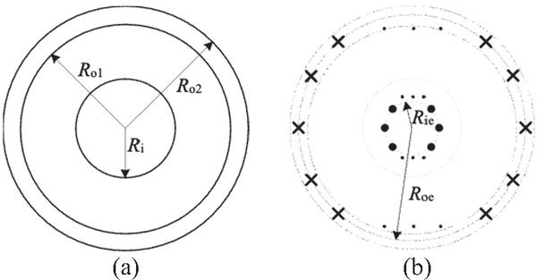
Figure 5 LCM for the coaxial cable: (a) cross-section of the coaxial cable and (b) decomposed line currents for the inner and outer conductors.

Therefore, the inner and outer conductors of the coaxial cable are decomposed into several line currents to determine the inductance deviation between the straightened case and bent cases, as shown in Fig. 5. The coaxial cable, with inner conductor of radius $R_{\mathrm{i}}$, outer conductor of inside radius $R_{\mathrm{o1}}$, and outside radius $R_{\mathrm{o2}}$, is equivalent to $n_{\mathrm{i}}$ line currents lying uniformly along the circle of radius $R_{\text{ie}}$ and $n_{\mathrm{o}}$ line currents lying uniformly along the circle of radius $R_{\mathrm{oe}}$. The following formulas are adopted to determine the equivalent radii:

$$R_{\mathrm{ie}}=\frac{R_{\mathrm{i}}}{2},$$	(22)
$$R_{\mathrm{oe}}=\frac{R_{\mathrm{o1}}+R_{\mathrm{o2}}}{2}.$$	(23)

During the calculation of the self-inductances for the inner and outer conductors, the mutual inductances among the decomposed line currents should be taken into account, and hence the self-inductances are:

$L_{11}^{\prime }$	$={\displaystyle \frac{1}{n_{\mathrm{i}}}}{L}_{11}+{\displaystyle \frac{1}{n_{\mathrm{i}}}}{\displaystyle \sum _{k=1}^{n_{\mathrm{i}}-1}}{M}_{\mathrm{i},k},$	(24)
$L_{22}^{\prime }$	$={\displaystyle \frac{1}{n_{\mathrm{o}}}}{L}_{22}+{\displaystyle \frac{1}{n_{\mathrm{o}}}}{\displaystyle \sum _{k=1}^{n_{\mathrm{o}}-1}}{M}_{\mathrm{o},k},$	(25)

where $L_{11}^{\prime }$ and ${\mathrm{L}}_{22}^{\prime }$ are the self-inductances of the inner and outer conductors of the coaxial cable, $L_{11}$ as well as $L_{22}(L_{11}=L_{22})$ is the self-inductance of a line current, and $M_{\mathrm{i},k}$ and $M_{\mathrm{o},k}$ are the mutual inductances between the two-line currents decomposed by the inner and outer conductor with the intervals of $k/n_i$ and $k/n_o$ circumference, respectively.

By regarding the inner and outer conductors as two complete line currents, their mutual inductance $M_{12}$ can be calculated with the equivalent distance of $R_{\mathrm{oe}}$.

To summarize, the inductance of the coaxial cable is:

$L$	$=L_{11}^{\prime }+L_{22}^{\prime }-2M_{12}$
	$={\displaystyle \frac{1}{n_{\mathrm{i}}}}{L}_{11}+{\displaystyle \frac{1}{n_{\mathrm{i}}}}{\displaystyle \sum _{k=1}^{n_{\mathrm{i}}-1}}{M}_{\mathrm{i},k}+{\displaystyle \frac{1}{n_{\mathrm{o}}}}{L}_{22}$
	$+{\displaystyle \frac{1}{n_{\mathrm{o}}}}{\displaystyle \sum _{k=1}^{n_{\mathrm{o}}-1}}{M}_{\mathrm{o},k}-2M_{12}$
	$=\left(L_{11}+L_{22}-2M_{12}\right)-{\displaystyle \frac{1}{2n_{\mathrm{i}}}}{\displaystyle \sum _{k=1}^{n_{\mathrm{i}}-1}}\left(2L_{11}-2M_{\mathrm{i},k}\right)$
	$-{\displaystyle \frac{1}{2n_{\mathrm{o}}}}{\displaystyle \sum _{k=1}^{n_{\mathrm{o}}-1}}\left(2L_{22}-2M_{\mathrm{o},k}\right),$	(26)

where every item in parentheses is the expression of the inductance for a parallel-pair cable in LCM.

It is worth noting that (3.2) applies to both straightened and bent coaxial cable layouts. In the straightened case, (3.1) is leveraged to compute the inductances. Moreover, in bent cases, (3.1) is utilized to estimate the inductances, in which the mutual inductances of the decomposed line currents are approximated by (19) despite the deviation of the relative positions.

The difference between the inductance of the bent coaxial cable and that of the straightened case yields the inductance deviation for the coaxial cable:

$L_{\mathrm{\Delta }\text{coa}}$	$={L_{\mathrm{\Delta }}|}_{d=R_{\mathrm{oe}}}-{{\displaystyle \frac{1}{2n_{\mathrm{i}}}}{\displaystyle \sum _{k=1}^{n_{\mathrm{i}}-1}}{L}_{\mathrm{\Delta }}|}_{d=r_{\mathrm{i},k}}$
	$-{{\displaystyle \frac{1}{2n_{\mathrm{o}}}}{\displaystyle \sum _{k=1}^{n_{\mathrm{o}}-1}}{L}_{\mathrm{\Delta }}|}_{d=r_{\mathrm{o},k}},$	(27)

where $L_{\mathrm{\Delta }}$ is the inductance deviation for the parallelpair cable obtained by (3.1):

$r_{\mathrm{i},k}$	$=2R_{\mathrm{ie}}\sin \left({\displaystyle \frac{k\pi }{n_{\mathrm{i}}}}\right),$	(28)
$r_{\mathrm{o},k}$	$=2R_{\mathrm{oe}}\sin \left({\displaystyle \frac{k\pi }{n_{\mathrm{o}}}}\right).$	(29)

4 NUMERICAL RESULTS AND DISCUSSION

The inductance deviation between the straightened layout and bent layouts for the parallel-pair cable and coaxial cable has been presented by a semi-analytical formula including non-closed-form expressions. In this section, the inductance deviation formula is solved for specific testing cases with numerical integration and compared with the results of the FEM. Then, the dependence of the inductance deviation on the parameters of the cable is investigated and the effect of the inductance deviation on realistic measurement of the lumped inductance is discussed. Besides, the frequency limitation of the semi-analytical formula and the measured inductance of a cable are also demonstrated to offer reference to realistic inductance measurement.

4.1 Comparison with FEM results

The inductance deviation between the straightened layout and the bent layouts in the angle from 0 to $11\pi /6$ of a parallel-pair consisting of two identical cylindrical conductors, with the parameters shown in Table 1, is calculated using (3.1), in which the non-closed-form integrals are handled by numerical integration. The corresponding three-dimensional FEM models are constituted in COMSOL Multiphysics software and solved by its Magnetic Fields, Current Only interface for the straightened layout and the bent layouts for the angle range $\pi /2:\pi /6:11\pi /6$, of which the geometry and conductor terminal meshes are shown in Figs. 6 (a), 6 (c), and 7 (a), respectively. The inductance deviation results of the semi-analytical method and FEM are illustrated in Fig. 8.

Table 1 Parameters of the parallel-pair cable

Cable	Conductor	Conductor
Length	Axis Distance	Radius
1 m	20 mm	5 mm

Table 2 Parameters of the coaxial cable

Cable	Inner	Outer
Length	Conductor	Conductor
	Radius	Inner Radius
1 m	5 mm	10 mm
Outer Conductor	Inner Conductor	Outer Conductor
Outer Radius	LCMs $(n_{\mathrm{i}})$	LCMs $\left(n_{\mathrm{o}}\right)$
12 mm	5	5

The inductance deviation of a coaxial cable with the parameters in Table 2 is also calculated by (27) and (3.1) and COMSOL Multiphysics FEM software, in which the outer conductor is represented by a solid tube. The geometry and conductor terminal meshes are demonstrated in Figs. 6 (b), 6 (d), and 7 (a), respectively. The results of the semi-analytical formula and FEM method are shown in Fig. 9.

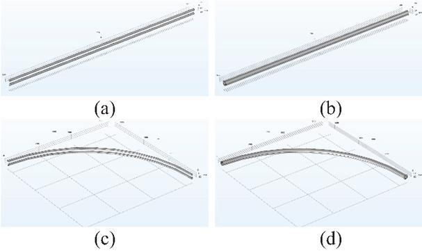
Figure 6 Geometry for the cable FEM models in COMSOL Multiphysics: (a) parallel-pair cable in the straightened layout, (b) coaxial cable in the straightened layout, (c) parallel-pair cable in the bent layout with ${\theta }_{\mathrm{m}}=\pi /2$, and (d) coaxial cable in the bent layout with ${\theta }_{\mathrm{m}}=\pi /2$.

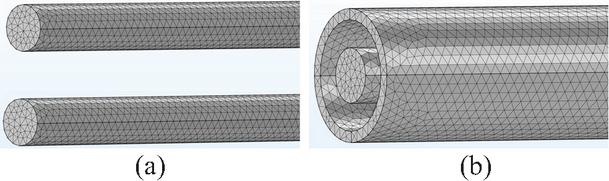
Figure 7 Meshing of the conductor terminals in COMSOL: (a) parallel-pair cable totally including 910324 mesh units for the straightened layout and (b) coaxial cable totally including 1178841 mesh units for the straightened layout.

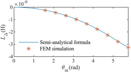
Figure 8 Comparison between the results of the proposed semi-analytical formula and the FEM for the parallel-pair cable.

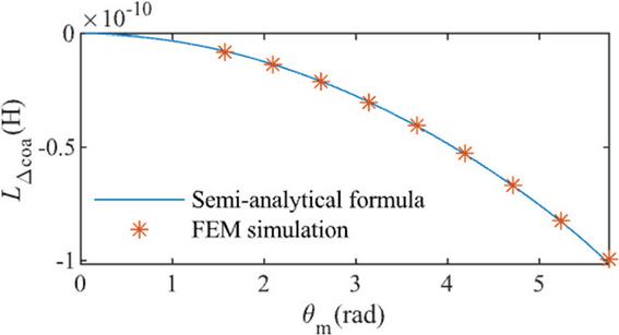
Figure 9 Comparison between the results of the proposed semi-analytical formula and the FEM for the coaxial cable.

It can be seen that the inductance deviation obtained by the proposed semi-analytical formula for both the parallel-pair cable and coaxial cable manifests remarkable consistency with the FEM results, proving the accuracy of the proposed formula. Moreover, the average consuming time for a single calculation by the proposed formula and the FEM method is demonstrated in Table 3, where the two methods are executed by MATLAB R2021b and COMSOL Multiphysics 6.0 on a computer with two Intel Xeon Golden 5520R 2.2 GHz CPUs and 120 GB RAM. It can be seen that the proposed semi-analytical formula shows prominent efficiency in comparison with the FEM method.

Table 3 Average consuming time for a single calculation

Cable	Parallel-Pair	Coaxial
Type	Cable	Cable
Proposed formula	1.344 ms	11.24 ms
FEM method	186.2 s	168.5 s

4.2 Dependence of the inductance deviation

The inductance deviations obtained in (3.1) and (27) demonstrate explicit dependence on the parameters of the parallel-pair and coaxial cables. The inductance deviation for a parallel-pair cable with different ${\theta }_{\mathrm{m}},l$, and $d$ is illustrated in Fig. 10. The absolute value of the inductance deviation shows a positive correlation with ${\theta }_{\mathrm{m}}$; larger ${\theta }_{\mathrm{m}}$ means more severe bending and consequently larger inductance deviation. The absolute value of the inductance deviation manifests a negative correlation with $l$, because a longer cable leads to larger distance and weaker magnetic field coupling between cable segments, which exceeds the effect of the additional length. Moreover, the absolute value of the inductance deviation is positively correlated with $d$, since larger $d$ contributes to less counteracting effect of the two opposite-current conductors and therefore less coupling between segments.

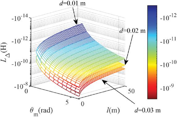
Figure 10 Dependence of the inductance deviation on the bending angle, length, and conductor distance for the parallel-pair cable.

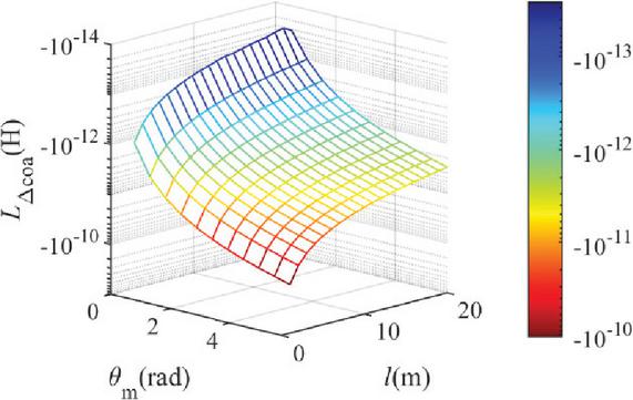
Figure 11 Dependence of the inductance deviation on the bending angle and length for the coaxial cable, with $R_{\text{oe}}=0.011\mathrm{m}$ and $R_{\mathrm{i}}=0.005\mathrm{m}$.

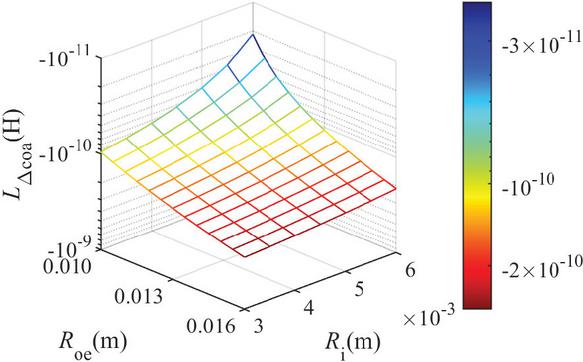
Figure 12 Dependence of the inductance deviation on the radii of the efficient inner and outer conductors for the coaxial cable, with ${\theta }_{\mathrm{m}}=11\pi /6$ and $l=1\mathrm{m}$.

The inductance deviation for a coaxial cable with different ${\theta }_{\mathrm{m}}$ and $l$ is illustrated in Fig. 11. Like a parallel-pair cable, the absolute value of the inductance deviation for a coaxial cable increases with ${\theta }_{\mathrm{m}}$ and decreases with $l$. Furthermore, as shown in Fig. 12, the absolute value of the inductance deviation demonstrates negative and positive correlations with $R_{\mathrm{i}}$ and $R_{\mathrm{oe}}$, respectively, in accordance with the relationship revealed by (27).

The number of decomposed line currents for the coaxial cable influences the accuracy and efficiency of the LCM. Figure 13 depicts the $L_{\mathrm{\Delta }{\mathrm{coa}}^{-}}-{\theta }_{\mathrm{m}}$ relationship with different $n_{\mathrm{i}}$ and $n_{\mathrm{o}}$ that are here taken as the same value for convenience. It can be seen that both the convergence and efficiency of the decomposition method are satisfying when $n_{\mathrm{i}}$ and $n_{\mathrm{o}}$ are equal to 5, while a greater decomposing number does not lead to apparently higher accuracy.

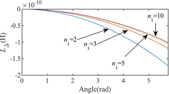
Figure 13 Dependence of the inductance deviation on the number of decomposed line currents for the coaxial cable, with $R_{\mathrm{i}}=0.005\mathrm{m},R_{\mathrm{oe}}=0.011\mathrm{m}$, and $l=1\mathrm{m}$.

4.3 Valid frequency range of the semi-analytical method

The semi-analytical method is proposed to deal with the effects of bending on cable inductance at low frequencies. In the deduction of the method, the lumped inductance of the cable is calculated to indicate the inductive part of the input impedance. Therefore, the proposed method is valid if the lumped model can represent the cable impedance, i.e., the cable is electrically short. The valid frequency of the method satisfies:

$$f\le \frac{v}{20l},$$

(30)

where $v$ is the propagation speed of electromagnetic wave along the cable, which is related to the structure and material of the cable. At higher frequencies, the input impedance of the cable cannot be represented by the lumped inductance such that the circuit model in Fig. 2 becomes invalid. Moreover, the quasi-static formulas for the partial inductance (2) and (3) are inaccurate at higher frequencies since the time delay shall be taken into account and the quasi-static approximation does not hold.

4.4 Inductance deviation in measurement

It is noted that the magnitude of the inductance deviation for a coaxial cable is quite small. For instance, in regard to a coaxial cable with $l=1\mathrm{m},R_{\mathrm{i}}=0.005\mathrm{m}$, $R_{\mathrm{oe}}=0.011\mathrm{m}$, and ${\theta }_{\mathrm{m}}=11\pi /6,L_{\mathrm{\Delta }\text{coa}}$ is equal to $-1.016\times {10}^{-10}\mathrm{H}$, of which the absolute value is smaller than the precision of most inductance measurement instrument.

According to Fig. 11, the absolute value of the inductance deviation for a longer cable is smaller than a shorter one. Regarding a coaxial with the same crosssection and bending angle as above but $l=10\mathrm{m}$, the inductance deviation reduces to $-6.874\times {10}^{-12}\mathrm{H}$, of which the absolute value is smaller than $1/10$ of the result with $l=1\mathrm{m}$. Moreover, the lumped inductance of a longer cable is larger than a shorter one, such that the inductance deviation between the straightened layout and bent layouts makes much less difference to the measurement results of the inductance. In brief, if a 10m coaxial cable is bent to a non-closed-arc for realistic lumped inductance measurement, the effect of bending on coaxial cable inductance is negligible.

The lumped inductance of three coaxial cable samples, with $l=1.0,3.0$, and 10.0 m, respectively, and the same cross-section that $R_{\mathrm{i}}=1.43\mathrm{mm}$ and $R_{\mathrm{oe}}=5.35$ mm, is measured using a HIOKI 3530-50 LCM meter at 50 Hz with different bending angles. The measurement results shown in Table 4 manifest no obvious relationship with the bending angles due to the stochastic noise of the LCM meter and the surrounding electromagnetic interference applied to the cable, where the effect of bending is drowned and immeasurable.

Table 4 Measured inductance at different bending angles for the coaxial cable with different length

Bending Angle	1 m	3.3 m	10 m
0	$0.232\mu \mathrm{H}$	$0.844\mu \mathrm{H}$	$2.95\mu \mathrm{H}$
$\pi /2$	$0.326\mu \mathrm{H}$	$0.660\mu \mathrm{H}$	$3.31\mu \mathrm{H}$
$\pi$	$0.287\mu \mathrm{H}$	$1.12\mu \mathrm{H}$	$2.93\mu \mathrm{H}$
$3\pi /2$	$0.184\mu \mathrm{H}$	$0.565\mu \mathrm{H}$	$3.41\mu \mathrm{H}$

5 CONCLUSION

A semi-analytical formula using the LCM is proposed in this paper for the bending effects on the inductance of the parallel-pair cable and then applied to the coaxial cable combined with the decomposition scheme of the conductors. The results demonstrate satisfying consistency with the inductance deviation extracted by the FEM method for both parallel-pair and coaxial cables.

The numerical results also show that the inductance of a parallel-pair or coaxial cable slightly decreases after bending and the deviation extends if the bending angle increases. The magnitude of the inductance deviation for a longer coaxial cable is small enough for instrument, indicating that the effect of non-closed-arc bending can be ignored in realistic measurement of the lumped coaxial cable inductance at low frequencies.

ACKNOWLEDGMENT

This work has been funded by the National Natural Science Foundation of China under grant No. 52377003.

APPENDIX 1

$L_{12\mathrm{b}}$ can be simplified by applying the change of variables ${\theta }_2-{\theta }_1=x$ and ${\theta }_2+{\theta }_1=y$:

$L_{12\mathrm{b}}$	$={\displaystyle \frac{{\mu }_0{R}^2}{4\pi }}{\displaystyle {\int }_0^{{\theta }_{\mathrm{m}}}}{\displaystyle {\int }_0^{{\theta }_{\mathrm{m}}}}{\displaystyle \frac{\cos ({\theta }_2-{\theta }_1)\mathrm{d}{\theta }_2\mathrm{d}{\theta }_1}{\sqrt{2R^2-2R^2\cos ({\theta }_2-{\theta }_1)+d^2}}}$
	$={\displaystyle \frac{{\mu }_0{R}^2}{8\pi }}[{\displaystyle {\int }_{-{\theta }_{\mathrm{m}}}^0}{\displaystyle \frac{\cos x}{\sqrt{2R^2-2R^2\cos x+d^2}}}{\displaystyle {\int }_{-x}^{x+2{\theta }_{\mathrm{m}}}}\mathrm{d}y\mathrm{d}x$
	$+{\displaystyle {\int }_0^{{\theta }_{\mathrm{m}}}}{\displaystyle \frac{\cos x}{\sqrt{2R^2-2R^2\cos x+d^2}}}{\displaystyle {\int }_{-x}^{x+2{\theta }_{\mathrm{m}}}}\mathrm{d}y\mathrm{d}x]$
	$={\displaystyle \frac{{\mu }_0{R}^2}{4\pi }}[{\displaystyle {\int }_{-{\theta }_{\mathrm{m}}}^0}{\displaystyle \frac{\left(x+{\theta }_{\mathrm{m}}\right)\cos x\mathrm{d}x}{\sqrt{2R^2-2R^2\cos x+d^2}}}$
	$+{\displaystyle {\int }_0^{{\theta }_{\mathrm{m}}}}{\displaystyle \frac{\left({\theta }_{\mathrm{m}}-x\right)\cos x\mathrm{d}x}{\sqrt{2R^2-2R^2\cos x+d^2}}}]$
	$={\displaystyle \frac{{\mu }_0{R}^2}{2\pi }}{\displaystyle {\int }_0^{{\theta }_{\mathrm{m}}}}{\displaystyle \frac{\left({\theta }_{\mathrm{m}}-x\right)\cos x\mathrm{d}x}{\sqrt{2R^2-2R^2\cos x+d^2}}}$
	$={\displaystyle \frac{{\mu }_0{l}^2}{2\pi {\theta }_{\mathrm{m}}}}{\displaystyle {\int }_0^{{\theta }_{\mathrm{m}}}}{\displaystyle \frac{\left({\theta }_{\mathrm{m}}-x\right)\cos x\mathrm{d}x}{\sqrt{2l^2-2l^2\cos x+d^2{\theta }_{\mathrm{m}}^2}}}$

REFERENCES

[1] “Coaxial communication cables – Part 1-114: Electrical test methods – Test for inductance,” IEC 61196-1-114:2015 [Online], Sep. 2015. Available: https://webstore.iec.ch/en/publication/23418.

[2] A. E. Ruehli, “Inductance calculations in a complex integrated circuit environment,” IBM Journal of Research and Development, vol. 16, no. 5, pp. 470–481, Sep. 1972.

[3] Z. Zhu, X. Xia, R. Streiter, G. Ruan, T. Otto, H. Wolf, and T. Gessner, “Closed-form formulae for frequency-dependent 3-D interconnect inductance,” Microelectronic Engineering, vol. 56, no. 3, pp. 359–370, Aug. 2001.

[4] G. Zhong and C.-K. Koh, “Exact closed-form formula for partial mutual inductances of on-chip interconnects,” in Proceedings IEEE International Conference on Computer Design: VLSI in Computers and Processors, pp. 428–433, Sep. 2002.

[5] Z. Y. Li, D. Y. Hu, Z. H. Yao, Y. W. Wang, Z. Y. Hong, K. Ryu, Y. H. Ma, and H. S. Yang, “Inductance evaluation of a $22.9\mathrm{kV}/50\mathrm{M}\mathrm{V}\mathrm{A}$ HTS cable with shield by electrical method,” in 2015 IEEE International Conference on Applied Superconductivity and Electromagnetic Devices (ASEMD), pp. 568–570, Nov. 2015.

[6] A. C. Silva and A. De Conti, “Calculation of the external parameters of overhead insulated cables considering proximity effects,” in 2017 International Symposium on Lightning Protection (XIV SIPDA), pp. 127–131, Oct. 2017.

[7] H. Li, R. Banucu, and W. M. Rucker, “Accurate and efficient calculation of the inductance of an arbitrary-shaped coil using surface current model,” IEEE Transactions on Magnetics, vol. 51, no. 3, pp. 1–4, Mar. 2015.

[8] J. T. Conway, “Exact solutions for the mutual inductance of circular coils and elliptic coils,” IEEE Transactions on Magnetics, vol. 48, no. 1, pp. 81–94, Jan. 2012.

[9] A. Ruehli, G. Antonini, and L. Jiang, Circuit Oriented Electromagnetic Modeling Using the PEEC Techniques. Hoboken, NJ: John Wiley & Sons, 2017.

BIOGRAPHIES

Xiao Chen was born in Yichang, China, in 1998. He received the B.Sc. and M.Sc. degrees in electrical engineering in 2020 and 2023, respectively, from the School of Electrical Engineering and Automation, Harbin Institute of Technology, Harbin, where he is currently pursuing a Ph.D. degree in electrical engineering. His research interests include transmission line theory, computational electromagnetics, and multiphysics field coupling simulations.

Haicheng Yin was born in Shanghai, China, in 1984. He graduated from Tongji University and holds a B.Sc. in EIE. He has been working for No. 23 Research Institute of CETC since 2008 and was appointed as an assistant chief engineer in 2020. His professional expertise lies in the international standardization work in the field of optical and electrical communication cable, connectors, and assemblies. He is an active member in the IEC community and has been project leader for 14 IEC standards. He was appointed as convenor for IEC/TC46/WG9 and IEC/SC46A/WG3, and as liaison for IEC/SC86A and IEC/ISO JTC3. For his outstanding work, he received an IEC 1906 award in 2022.

Gang Zhang was born in Tai’an, China, in 1984. He received the B.S. degree in electrical engineering from China University of Petroleum, Dongying, in 2007, and the M.S. and Ph.D. degrees in electrical engineering from Harbin Institute of Technology (HIT), Harbin, in 2009 and 2014, respectively. He is currently a Professor of Electrical Engineering with HIT. His research interests include electrical contact theory, uncertainty analysis of electromagnetic compatibility, and validation of CEM.

Francesco de Paulis was born in L’Aquila, Italy, in 1981. He received the Specialistic Laurea (summa cum laude) degree in electronic engineering from the University of L’Aquila (UAq), L’Aquila, in 2006, the M.S. degree in electrical engineering from Missouri University of Science and Technology, Rolla, MO, USA, in 2008, and the Ph.D. degree in electrical and information engineering from UAq in 2012. He is currently a Senior Research Professor with the UAq EMC Laboratory. His main research interests include the design of high-speed signals on PCBs, packages, and chips, RF interference in mixed-signal systems, and EMI problem investigation on PCBs.

Xin He was born in Wenshan, China, in 1996. He received the B.S. and M.Sc. degrees in electrical engineering from Harbin Institute of Technology (HIT), Harbin, in 2019 and 2021, respectively. He is currently pursuing a Ph.D. degree in electrical engineering with HIT, Shenzhen. His research interests include cable fault detection location and electromagnetic compatibility analysis.

ACES JOURNAL, Vol. 40, No. 12, 1206–1214
DOI: 10.13052/2025.ACES.J.401208
© 2026 River Publishers