Inversion Method Based on CNN-BiLSTM-Attention for SQUID TEM Data with IP Effect
Yanju Ji1, 2, Jinxiu Yuan1, Hui Luan1, 2, Yuan Wang1, 2, and Qiong Wu1, 2*
1College of Instrumentation and Electrical Engineering
Jilin University, Changchun 130026, China
jiyj@jlu.edu.cn, yuanjx6522@mails.jlu.edu.cn, luanhui@jlu.edu.cn, wangyuan_ciee@jlu.edu.cn, wuqiong_515@sina.cn*
2State Key Laboratory of Deep Earth Exploration and Imaging
Jilin University, Changchun 130026, China
Submitted On: April 29, 2025; Accepted On: December 23, 2025
Abstract
The superconducting quantum interference device time-domain electromagnetic (SQUID TEM) method has been widely used for the exploration of geological and mineral resources. Extracting resistivity and polarizability from TEM data aids in delineating subsurface metallic mineralization. However, traditional inversion methods are computationally intensive and slow. We propose an inversion method based on a convolutional neural network and bidirectional long short-term memory with attention (CNN-BiLSTM-Attention) to extract resistivity and polarizability of polarizable media from SQUID TEM data acquired with a magnetic source. The method combines the advantages of CNN for automatic feature extraction with the capabilities of BiLSTM for processing temporal data. Additionally, it incorporates an attention mechanism that emphasizes the extraction of key polarization features, thereby optimizing the parameters extraction process. The method can effectively extract resistivity and polarizability from SQUID TEM data. It is validated by the TEM data of theoretical models, and the errors of CNN-BiLSTM-Attention inversion results are smaller than that of the BiLSTM and CNN-LSTM methods.
Index Terms: Attention mechanism, BiLSTM, CNN, inversion method, polarizable medium, SQUID TEM.
I. INTRODUCTION
The lack of mineral resources resulting from socio-economic development may adversely affect global economic stability. To guarantee resource security and sustainable economic development, it is essential to advance deep earth exploration technologies for the precise identification of mineral resources [1]. These minerals typically exist in the form of sulfide or disseminated ores, which may cause an induced polarization (IP) effect. Resistivity and polarizability are two essential characteristics that affect the electromagnetic effect, and they indicate the positions of the ore bodies which are vital for the identification of metallic ores [2, 3]. Advancing inversion techniques can improve both accuracy and speed, which will in turn support secure and efficient mineral resource exploration through TEM inversion.
To detect exceedingly weak electromagnetic field signals, numerous researchers have studied superconducting quantum interference devices (SQUID), which are highly sensitive magnetic sensors capable of detecting magnetic field variations on the order of [4]. Superconducting quantum interference devices time domain electromagnetic (SQUID TEM) detection method has been extensively utilized in the investigation of geological and mineral resources. In practical exploration, TEM responses may exhibit sign reversal, a phenomenon commonly attributed to the polarization effect of the subsurface medium [5, 6, 7]. Consequently, it is essential to investigate the inversion method for electromagnetic induction-polarization (EM-IP) effect. In recent years, there have been numerous investigations into the extraction of the relevant polarization parameters. Viezzoli et al. inverted time-domain airborne electromagnetic IP parameters using a 1D lateral constraint method, showing that when the time constant is within a certain range, the method provides good solutions for both resistivity and polarizability [8]. Man et al. proposed an inversion method for airborne TEM data with IP effect based on Pearson correlation constraints, improving the accuracy and stability of the inverted resistivity and polarizability, and reducing inversion non-uniqueness [9]. Lu et al. presented a quasi-2-D inversion scheme for extracting resistivity and IP parameters from semi-airborne TEM data, improving inversion stability and recovering underground property distributions [10]. Wang et al. introduced a modified quasi-2D regularized Newton inversion scheme for extracting IP parameters of ColeCole model [11].
Conventional parameter-extraction methods often rely on an initial model and iterative solvers, making them computationally intensive and time-consuming. This poses a significant challenge in achieving a balance between efficiency and accuracy, especially when handling large-scale geophysical data. The neural networks have become a promising solution of geophysical problems, such as exploration geophysics, Earth system analysis [12, 13]. Ji et al. presented a neural network method using Rademacher complexity to accurately invert ground-source airborne TEM data for resistivity and roughness in rough geological media [14]. Alyousuf and Li presented a physics-based neural network inversion method that combines deterministic and neural network approaches [15]. Li et al. developed a probabilistic seismic petrophysical inversion method using a physics-informed neural network (PINN), improving accuracy and quantifying model uncertainty in predicting petrophysical properties from seismic data [16]. Neural networks, through extensive learning from vast amounts of training data, are capable of performing inversion without explicitly calculating the forward model, significantly reducing the computational complexity inherent in traditional methods. At the same time, the powerful learning capability and excellent generalization ability of neural networks enable them to provide higher parameter extraction accuracy and faster computational speeds when addressing various types of geophysical problems. This method enhances parameter extraction efficiency and expands its potential application in intricate geological settings.
We propose an attention-based CNN-BiLSTM inversion method to extract polarization parameters from SQUID TEM data acquired with a magnetic source. This method can leverage the benefits of convolutional neural network (CNN) in automatic feature extraction, combined with the capacity of bidirectional long short-term memory networks (BiLSTM) to capture temporal data and geographical context. Moreover, by integrating the attention mechanism, the model may autonomously concentrate on essential aspects within the input data. This method streamlines the parameter extraction process, dramatically improving both accuracy and speed. The method shows improved generalization and broader application potential compared with existing approaches.
II. NUMERICAL SIMULATION METHOD OF THE TIME-DOMAIN EM-IP RESPONSE
A. Numerical simulation method
Several physical models describe the polarization behavior of rocks. Notable instances encompass the Debye model, the Dias model, and the GEMTIP model, among others. The Cole-Cole complex resistivity model [17], introduced by Pelton et al. in 1978, is a typical approach and is articulated as follows:
| (1) |
where is dc resistivity, is polarizability, is time constant, is frequency-dependent coefficient, is imaginary unit, and is angular frequency.
This study assumes a layered medium model, and the magnetic source with a radius of positioned at the horizontal surface. The formula for the vertical magnetic field in the frequency domain is expressed as [18, 19]:
| (2) |
where is source-current amplitude, is first-order Bessel function, is reflection coefficient determined by the geoelectric parameters, , is wave number of the polarization medium, especially , is permeability of the medium, and represents integrable variable quantity of the Hankel transform. The frequency-domain electromagnetic response is derived using the Hankel transform. The vertical component of the induced voltage is calculated by the equation: . The frequency-domain results are subsequently converted to the time-domain using Guptasarma’s numerical linear filtering approach.
B. Validation of numerical simulation methods
Figure 1 presents the schematic diagram of the SQUID TEM system, which intuitively illustrates the geometric configuration and parameter settings of the system. The transmitter loop with a radius of 100 m is placed on the ground surface, and the SQUID receiver (Rx) is located at the center of the loop to measure the TEM response. The subsurface is represented by a horizontally layered geoelectric model, where each layer is characterized by its resistivity and polarizability parameters based on the Cole-Cole model. In SQUID TEM system, the transmitter emits a bipolar square wave current, and the SQUID receiver collects TEM responses containing underground information. Figure 2 displays the electromagnetic response of half-space model with the resistivity at 100 , and the numerical simulation results nearly coincide with the analytical solution. The relative error is below 1.2%, and the accuracy of the numerical simulation method is verified.
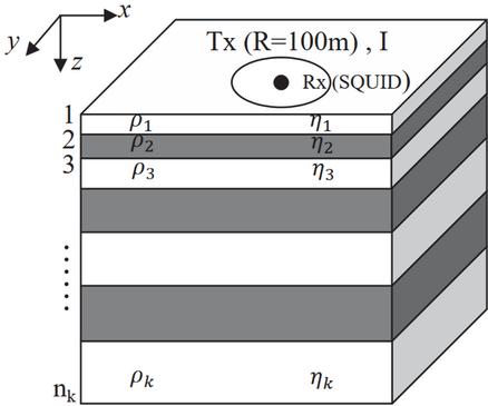
Figure 1 Configuration of SQUID TEM system.
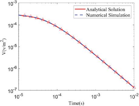
Figure 2 Numerical simulation results of electromagnetic response of half-space model.
C. Polarizable medium parameters characteristics
The Cole-Cole model of a polarizable medium comprises four parameters: resistivity , polarizability , time constant , and frequency-dependent coefficient . The time-domain EM-IP effect may be significantly affected by the resistivity and polarizability. The time-domain EM-IP effect of magnetic source of varying resistivities and polarizabilities is calculated. The TEM response curves presented in this paper represent the results after taking the absolute values. Figure 3 illustrates the TEM responses for resistivities of 10,100, and 1000 , with a polarizability . In Fig. 3, it can be seen that the effect of different resistivities on the electromagnetic response exhibits a clear difference in the time and amplitude characteristics [20]. When resistivity is low (e.g., blue curve, ), the decay of the response curve is slower, the negative response appears later, and the amplitude of the negative response is larger; conversely, as resistivity increases (e.g., the red curve, and the yellow curve, ), the decay of the electromagnetic response is markedly expedited, the negative response emerges sooner, and the amplitude progressively diminishes. Figure 4 shows the electromagnetic response corresponding to resistivity and polarizability . The differences in polarizability significantly affect electromagnetic responses, particularly in the timing and amplitude features of negative responses. When the polarizability is low (e.g., blue curve, ), the negative response occurs at a later stage, and its magnitude is relatively reduced. Conversely, as the polarizability escalates (e.g., red curve, and yellow curve, ), the negative response manifests sooner, while the magnitude progressively intensifies.
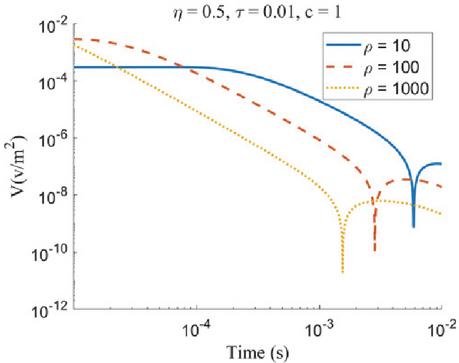
Figure 3 Electromagnetic response curves for different resistivities.
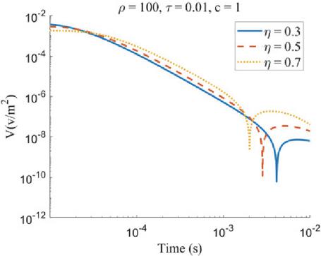
Figure 4 Electromagnetic response curves for different polarizabilities.
III. CNN-BiLSTM-ATTENTION INVERSION METHOD FOR EM-IP EFFECT
A. Convolutional neural network
The basic architecture of CNN comprises a convolutional layer, a pooling layer, and a fully connected layer, as illustrated in Fig. 5. The convolutional layer enables the extraction of local features from the input data via convolutional operations, thereby efficiently collecting essential patterns and structural information in the time series data of the EM-IP effect [21]. The pooling layer utilizes maximum pooling to reduce computing requirements and improve feature stability. The ReLU activation function is utilized to exclude insignificant data and improve the network’s nonlinear representation. The precise formulation of the ReLU activation function is .
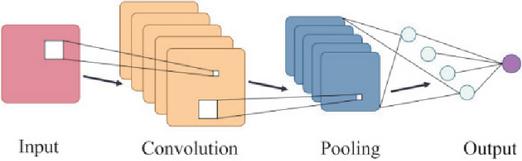
Figure 5 Convolutional neural network architecture diagram.
B. Bidirectional long short-term memory network
Long short-term memory (LSTM) networks effectively handle time series data by integrating longterm and short-term memories via a gating mechanism [22]. Figure 6 illustrates the cellular architecture of LSTM.
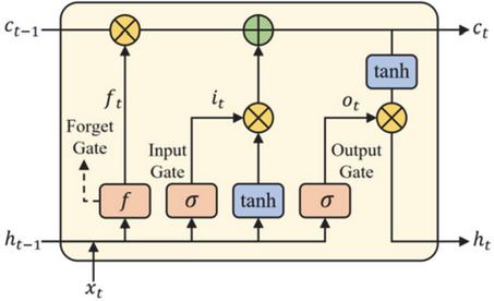
Figure 6 Diagram of the internal structure of the long short-term memory.
In Fig. 6, represents the previous cell state, is the prior hidden state, and is the current input. The forget gate determines which information from is discarded, while the relevant information is passed to . The input gate controls how much of the current input is retained, and the output gate regulates the transfer of information from the current cell state to the output .
BiLSTM enhances the conventional unidirectional LSTM. A conventional LSTM analyzes historical data in a single direction and cannot leverage future information. The BiLSTM, through its unique gating mechanisms and bidirectional processing capability, can simultaneously learn the temporal dependencies of this feature sequence from both the forward and reverse directions [23]. This capability is particularly advantageous for analyzing the temporal data of the EM-IP effect, as it comprehensively captures temporal relationships, amalgamates historical and future information, optimizes the training process, and enhances the accuracy of parameters extraction. The structure is illustrated in Fig. 7.
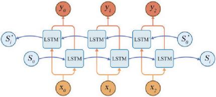
Figure 7 Diagram of the structure of Bi-LSTM.
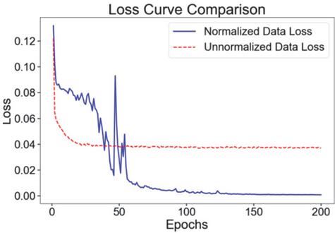
Figure 9 Overall framework of CNN-BiLSTM-Attention.
C. Attention mechanism
The attention mechanism is a bio-inspired selective processing method that emulates the human visual system’s ability to focus on critical information. In the context of sequence modeling, it facilitates a weighted aggregation of features across all time steps by learning a set of normalized weights, thereby enabling the network to automatically emphasize the most task-relevant segments [24]. To enhance the efficiency of parameter extraction from EM-IP data, this study employs a soft attention mechanism. This allows the model to concentrate its computational resources on the most information-rich temporal segments while suppressing diffuse background signals. Let the matrix represent the hidden state sequence from the BiLSTM, where is the matrix space of real-valued elements with rows and columns. Consequently, the state at the -th time step, is a dimensional column vector, and the total sequence length is . The attention is computed as follows:
| (3) | |
| (4) | |
| (5) |
where is trainable weight matrix, is normalized attention weight vector, and is resulting context vector which aggregates the sequence information. The soft attention mechanism adaptively emphasizes the late-time windows that are most sensitive to polarizability by assigning higher weights to the corresponding time steps. The SoftMax normalization effectively suppresses noise and early-time transmitter interference by assigning them extremely low weights, thereby reducing the prediction variance. Concurrently, the attention weight vector provides an interpretable map of temporal importance.
D. Data preprocessing
An essential step in the successful extraction of parameters is data preparation. This procedure involves applying normalization to input and output data in order to adjust them [25]. To reduce the effect of training bias caused by differences in numerical ranges, different electromagnetic response magnitudes are normalized to a constant range in the input data. For EM-IP effect data with a time series structure, this is very important. To improve forecast accuracy, the output data of polarizability and resistivity are also normalized. In bidirectional LSTM networks, normalization takes on a special importance. It avoids the vanishing or ballooning gradients that result from data that has not been normalized. Moreover, it improves accuracy and makes model convergence easier. Figure 8 present the loss curves for unnormalized and normalized data. The loss curve for the normalized data exhibits faster convergence and a lower final loss, thereby demonstrating the significant improvement in training efficiency and convergence performance afforded by normalization.
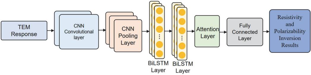
Figure 8 Loss curve comparison.
E. CNN-BiLSTM-Attention inversion method
Figure 9 illustrates the overall architecture of the CNN-BiLSTM-Attention inversion framework proposed in this paper. Its core concept lies in a multistage, multi-dimensional feature extraction and focusing process, designed to achieve a deep analysis of the complex non-linear relationship between the transient electromagnetic (TEM) response data and the parameters of resistivity () and polarizability (). It establishes a hierarchical “local-global-focus” analysis pipeline. The convolutional layers extract local patterns, the BiLSTM models bidirectional dependencies, and the attention layer re-weights the sequence according to to generate the context vector . Finally, the resistivity and polarizability are estimated. This method circumvents the drawbacks of traditional inversion methods, which are dependent on an initial model, computationally intensive, and may converge to local optima. The advantage of this framework stems from the functional complementarity of its components and its progressive, intelligent analysis capability.
The process commences with a one-dimensional CNN. In geophysical inversion, the local morphology of the TEM response curve across different time channels contains a wealth of geoelectric information. The CNN layers, through their convolutional kernels, can efficiently capture these local, fundamental feature patterns. This serves as an effective feature “preprocessing” and dimensionality reduction of the original high-dimensional time-series signal, laying a solid foundation for the more complex temporal analysis that follows.
The feature sequence extracted by the CNN is fed into a BiLSTM. The EM-IP effect is inherently a dynamic process that spans the entire time window, with long-range dependencies existing between signals at different time points. The BiLSTM, through its unique gating mechanisms and bidirectional processing capability, can simultaneously learn the temporal dependencies of this feature sequence from both the forward and reverse directions. Compared to a unidirectional LSTM or a traditional recurrent neural network, the BiLSTM can more comprehensively understand the contextual relationships within the signal, thereby achieving a more profound grasp of the overall dynamic evolution of the TEM response.
Finally, introduction of the Attention mechanism is a key optimization for the model and represents the core advantage of this architecture over other hybrid models. In a complex TEM response, not all temporal data points are of equal importance to the final parameter prediction. For instance, the negative-value region where the polarization effect occurs or the inflection points of the decay curve often contribute more significantly to the inversion result. The attention mechanism can, based on the hidden states output by the BiLSTM layer, dynamically assign different weights to the features of each time step. This allows the model to “focus” on those signal segments that are most sensitive to resistivity and polarizability and are most information-rich, while simultaneously suppressing noise and irrelevant information. This focusing capability is critical for enhancing the model’s accuracy and robustness.
IV. KEY PARAMETER SETTINGS OF CNN-BiLSTM-ATTENTION
In the CNN-BiLSTM-Attention framework, the selection of critical parameters, including the initial learning rate and Dropout value, significantly influences the model’s performance, particularly for parameters extraction efficacy. Therefore, to guarantee that the model is trained under ideal conditions and attains high accuracy, this study systematically picks and optimizes critical hyperparameters [26].
A. Dropout value setting
During the training of deep neural networks, a small dataset combined with a complex model can lead to overfitting. This is primarily indicated by a higher loss function on the test dataset compared to the training set, along with reduced prediction accuracy relative to the training set. Dropout mitigates overfitting by randomly deactivating neurons during training [27].
The selection of the Dropout value will yield varying impacts on the training process. This paper selects Dropout values of 0.0001, 0.001, 0.01, and 0.1 for comparison. The test results, illustrated in Fig. 10, indicate that the loss function decreases most rapidly at a Dropout value of 0.001, yielding the smallest final loss function value. Consequently, the optimal Dropout value for this study is determined to be 0.001 for the CNN-BiLSTM-Attention inversion method.
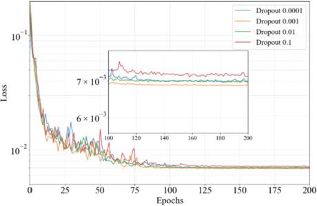
Figure 10 Comparison of loss curves at different Dropout values.
B. Initial learning rate selection
This paper employs Adam’s adaptive learning rate strategy, which adjusts the learning rate depending on current and historical gradient information [28]. A high initial learning rate can enhance training efficiency; nevertheless, an excessively high learning rate may bypass the global optimum or result in gradient explosion, preventing convergence. Figure 11 illustrates the comparison of loss curves corresponding to various beginning learning rates. With an initial learning rate of 0.1, the loss function nearly ceases to decrease after one training iteration, resulting in a gradient explosion; conversely, the final value of the loss function is minimized and most stable at a learning rate of 0.01.
Following the optimization and study of additional parameters, we established the definitive key parameter settings, with the particular values and corresponding settings detailed in Table 1. The neural network exhibited superior performance, and the model functioned effectively to obtain the most dependable inversion results.
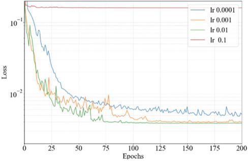
Figure 11 Comparison of loss curves at different initial learning rates.
Table 1 Neural network key parameter settings
| Neural Network Parameters | Values |
| CNN Convolutional Layer Kernel Size | 2 |
| CNN Convolutional Layer Count | 2 |
| BiLSTM Hidden Layer Node Count | 64 |
| BiLSTM Layer Count | 2 |
| Learning Rate Optimization Algorithm | Adam |
| Dropout Value | 0.001 |
| Initial Learning Rate | 0.01 |
V. THEORETICAL MODEL VERIFICATION
To validate the efficacy of the CNN-BiLSTMAttention inversion method, theoretical models are developed for method verification.
A. Dataset, training strategy
This paper designs three models, a polarizable halfspace, a three-layer polarizable model and a five-layer polarizable model. For all models, the time constant and the frequency-dependent coefficient are kept consistent, with a time constant of 0.01 and a frequency-dependent coefficient of 1, to ensure the comparability of results across different geometric complexities. We generate parameter combinations centered around the baseline parameters of each theoretical model within a range of 25% to 200%. Resistivity () is sampled using logarithmic equal-ratio steps, while polarizability () is sampled with linear equal-distance steps. Based on this, the corresponding TEM response data are generated to form the complete sample datasets.
The sample datasets are divided into training, validation, and test sets (70%, 15%, 15%). Furthermore, all input TEM response data and output parameter labels are normalized to eliminate dimensional differences and accelerate model convergence. The optimization objective of the model training is to minimize the Mean Squared Error (MSE) between the predicted parameters and the true theoretical parameters, using the Adam adaptive moment estimation optimizer for the iterative updating of model weights. To prevent model overfitting and achieve stable convergence, we designed a combined convergence criterion. The core of this criterion consists of an Early Stopping mechanism and a dynamic learning rate decay strategy. The Early Stopping mechanism monitors the validation set loss; when it does not improve for 25 consecutive epochs, the training is automatically terminated, and the model weights that performed best on the validation set are restored. Concurrently, if the validation set loss stagnates for 15 epochs, the learning rate is automatically reduced to 0.5 times its previous value, with a minimum learning rate of , then the model may perform a finer search when approaching an optimum.
B. Polarizable half-space model
We extract the parameters from TEM data for the polarizable half-space model. The polarizable halfspace model is configured with polarizability ranging from 0.1 to 0.9, resistivity from 1 to 1000 , a time constant , and a frequency-dependent coefficient . The TEM responses are calculated and the sample set is obtained.
Considering the correlation between resistivity and polarizability, the joint extraction error of the two parameters provides a more thorough indication of the correctness of the parameter extraction. In the computation of the combined relative error, resistivity and polarizability are assigned equal weight. To assess the accuracy of the extraction method, Fig. 12 displays the relative errors of the joint parameters extraction for various resistivity and polarization combinations, with their distribution illustrated through color coding. The relative error of the combined extraction results remains below 4% for all combinations of resistivity and polarizability. The effectiveness of the CNN-BiLSTMAttention inversion method is verified.
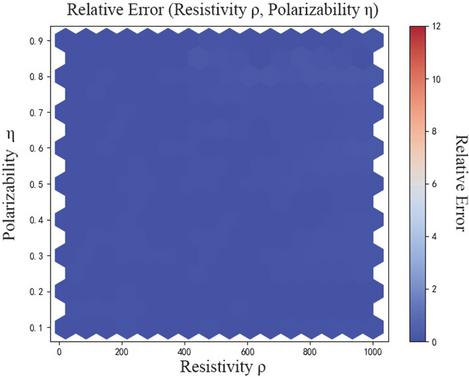
Figure 12 Joint relative error of resistivity and polarizability extraction.
C. Three-layer polarizable model
To further validate the effectiveness of the CNN-BiLSTM-Attention inversion method, this study conducts verification on the resistivity and polarizability extraction of a three-layer polarizable model. The thickness of each layer, and the resistivity and polarizability of the theoretical model are presented in Table 4. The polarizable medium models are developed, and the TEM response is computed as the sample set, followed by the application of the neural network for parameters extraction. Furthermore, we applied BiLSTM and CNN-LSTM to invert the TEM response of the layered model, and a comparison of their inversion accuracies is presented in the tables.
To more clearly evaluate the performance of the neural network inversion at the time-series level, we quantify it from three complementary dimensions: absolute error energy, mean absolute deviation, and relative percentage deviation, using the Root Mean Square Error (RMSE), Mean Absolute Error (MAE), and Mean Absolute Percentage Error (MAPE), respectively. The following metrics are all calculated on the absolute-valued waveforms to avoid the impact of sign reversals on the evaluation.
The RMSE, as defined in equation (6), holistically measures the “energy” of the error and is more sensitive to larger deviations, which facilitates the perception of significant mismatches occurring in critical time windows:
| (6) |
MAE, as defined in equation (7), measures the overall deviation as the average of the absolute differences; it is both intuitive and robust, which facilitates direct comparison across different datasets.
| (7) |
MAPE, as defined in equation (8), characterizes the relative amplitude deviation in percentage terms, making it well-suited for the characteristics of TEM data, which decay across several orders of magnitude.
| (8) |
Tables 2 and 3 present a detailed comparison of these performance metrics for the inversion of resistivity and polarizability, respectively. The results show that the CNN-BiLSTM-Attention model consistently outperforms the other two models across all metrics. For both resistivity and polarizability, it achieves the lowest RMSE, MAE, and MAPE values, indicating higher prediction accuracy and stability. This quantitative analysis further confirms the superiority of the proposed model.
Table 2 Comparison of resistivity inversion accuracy using different methods
| Method | RMSE | MAE | MAPE (%) |
| CNN-BiLSTM-Attention | 16.23 | 12.15 | 5.57 |
| BiLSTM | 33.85 | 28.12 | 13.05 |
| CNN-LSTM | 31.43 | 26.35 | 15.24 |
Table 3 Comparison of polarizability inversion accuracy using different methods
| Method | RMSE | MAE | MAPE (%) |
| CNN-BiLSTM-Attention | 0.035 | 0.028 | 6.75 |
| BiLSTM | 0.078 | 0.065 | 15.32 |
| CNN-LSTM | 0.069 | 0.057 | 16.54 |
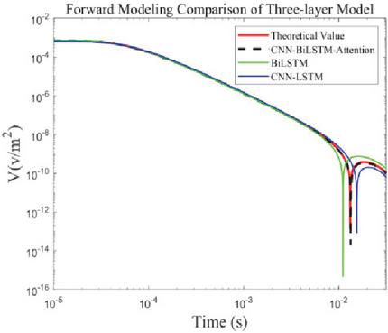
Figure 13 Comparison of the inversion TEM response and theoretical response for the three-layer model.
The TEM response of the inversion results is compared with the theoretical response, as illustrated in Fig. 13. This figure clearly demonstrates that the inversion results of the CNN-BiLSTM-Attention model exhibit the highest correlation between the TEM response and the theoretical response, signifying that the model adeptly captures the characteristics of the electromagnetic response and is suitable for resistivity and polarizability parameters extraction. Tables 4–6 present the inversion results for the CNN-BiLSTMAttention, BiLSTM, and CNN-LSTM methods, respectively. The CNN-BiLSTM-Attention model demonstrates a significant advantage in both the accuracy and stability of parameter extraction. It achieves a highly precise extraction of resistivity and polarizability across all layers, with the relative errors of the extracted parameters consistently below 6.5%, thereby validating the effectiveness of the CNN-BiLSTM-Attention method.
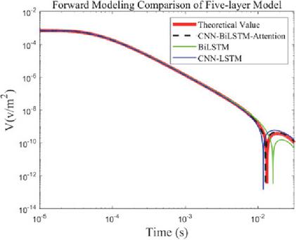
Figure 14 Comparison of the inversion TEM response and theoretical response for the five-layer model.
Table 4 CNN-BiLSTM-Attention model
| Layer | Thickness | Theoretical | Extracted | Relative Error | Theoretical | Extracted | Relative Error |
| (m) | Resistivity | Resistivity | in Resistivity | Polarizability | Polarizability | in Polarizability | |
| (m) | (m) | (%) | (%) | ||||
| Layer1 | 100 | 100 | 103.97 | 3.97 | 0.1 | 0.0968 | 3.20 |
| Layer2 | 100 | 10 | 10.65 | 6.50 | 0.6 | 0.6341 | 5.68 |
| Layer3 | INT | 100 | 102.93 | 2.93 | 0.2 | 0.2096 | 4.80 |
Table 5 BiLSTM model
| Layer | Thickness | Theoretical | Extracted | Relative Error | Theoretical | Extracted | Relative Error |
| (m) | Resistivity | Resistivity | in Resistivity | Polarizability | Polarizability | in Polarizability | |
| (m) | (m) | (%) | (%) | ||||
| Layer1 | 100 | 100 | 92.18 | 7.82 | 0.1 | 0.0878 | 12.20 |
| Layer2 | 100 | 10 | 11.23 | 12.30 | 0.6 | 0.6823 | 13.72 |
| Layer3 | INT | 100 | 108.93 | 8.93 | 0.2 | 0.2338 | 16.90 |
Table 6 CNN-LSTM model
| Layer | Thickness | Theoretical | Extracted | Relative Error | Theoretical | Extracted | Relative Error |
| (m) | Resistivity | Resistivity | in Resistivity | Polarizability | Polarizability | in Polarizability | |
| (m) | (m) | (%) | (%) | ||||
| Layer1 | 100 | 100 | 106.27 | 6.27 | 0.1 | 0.1083 | 8.30 |
| Layer2 | 100 | 10 | 9.13 | 8.70 | 0.6 | 0.5078 | 15.37 |
| Layer3 | INT | 100 | 111.97 | 11.97 | 0.2 | 0.1738 | 13.10 |
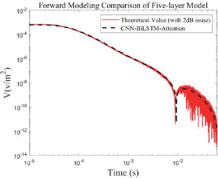
Figure 15 Forward modeling comparison for the fivelayer model with added noise.
Table 7 CNN-BiLSTM-Attention model
| Layer | Thickness | Theoretical | Extracted | Relative Error | Theoretical | Extracted | Relative Error |
| (m) | Resistivity | Resistivity | in Resistivity | Polarizability | Polarizability | in Polarizability | |
| (m) | (m) | (%) | (%) | ||||
| Layer1 | 200 | 100 | 100.54 | 0.54 | 0.1 | 0.1047 | 4.7 |
| Layer2 | 100 | 75 | 78.46 | 4.61 | 0.3 | 0.3217 | 7.23 |
| Layer3 | 50 | 50 | 51.67 | 3.34 | 0.6 | 0.6118 | 1.96 |
| Layer4 | 100 | 75 | 71.94 | 4.08 | 0.3 | 0.3133 | 4.43 |
| Layer5 | INT | 500 | 531.27 | 6.25 | 0.1 | 0.1051 | 5.10 |
Table 8 BiLSTM model
| Layer | Thickness | Theoretical | Extracted | Relative Error | Theoretical | Extracted | Relative Error |
| (m) | Resistivity | Resistivity | in Resistivity | Polarizability | Polarizability | in Polarizability | |
| (m) | (m) | (%) | (%) | ||||
| Layer1 | 200 | 100 | 103.06 | 3.06 | 0.1 | 0.1135 | 13.5 |
| Layer2 | 100 | 75 | 78.92 | 5.23 | 0.3 | 0.3299 | 9.96 |
| Layer3 | 50 | 50 | 43.45 | 13.10 | 0.6 | 0.6649 | 10.81 |
| Layer4 | 100 | 75 | 68.93 | 8.09 | 0.3 | 0.2567 | 14.43 |
| Layer5 | INT | 500 | 598.88 | 19.77 | 0.1 | 0.1182 | 18.20 |
Table 9 CNN-LSTM model
| Layer | Thickness | Theoretical | Extracted | Relative Error | Theoretical | Extracted | Relative Error |
| (m) | Resistivity | Resistivity | in Resistivity | Polarizability | Polarizability | in Polarizability | |
| (m) | (m) | (%) | (%) | ||||
| Layer1 | 200 | 100 | 96.16 | 3.84 | 0.1 | 0.0829 | 17.1 |
| Layer2 | 100 | 75 | 80.64 | 7.52 | 0.3 | 0.2771 | 7.63 |
| Layer3 | 50 | 50 | 55.17 | 10.34 | 0.6 | 0.4883 | 18.61 |
| Layer4 | 100 | 75 | 76.9 | 2.53 | 0.3 | 0.3253 | 8.43 |
| Layer5 | INT | 500 | 546.37 | 9.274 | 0.1 | 0.1113 | 11.30 |
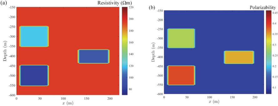
Figure 16 Polarizable anomalies theoretical model.
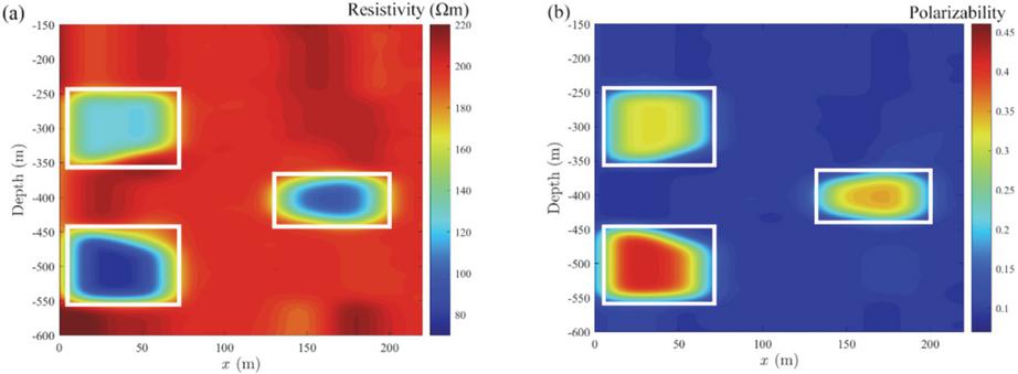
Figure 17 Inversion result of polarizable anomalies.
D. Five-layer polarizable model
In order to further assess the feasibility of the method, we selected a typical five-layer polarizable model for parameters extraction. The thickness of each layer, along with the parameter settings for resistivity and polarizability, is presented in Table 7. The CNN-BiLSTM-Attention, BiLSTM, and CNN-LSTM inversion methods were employed to extract the parameters from the TEM responses of the five-layer polarizable medium model, respectively. Figure 14 compares the TEM responses derived from various parameters extraction methods against the theoretical response. It is evident that the TEM response from the CNN-BiLSTM-Attention method exhibits the greatest concordance with the theoretical response, signifying its superior performance in parameters extraction. The inversion results are presented in Tables 7–9, indicating that the relative errors for the CNN-BiLSTM-Attention approach are less than 7.3%, demonstrating superior accuracy and stability compared to alternative methods.
To further verify the stability of the inversion method proposed in this paper, we conducted an antinoise test. We added Gaussian white noise to the theoretical TEM response data of the five-layer model, with the SNR of 2 dB. We used the noisy theoretical TEM response as input to the CNN-BiLSTM-Attention model for inversion. A comparison between the forward response of the inversion results and the noisy theoretical response is shown in Fig. 15. As can be seen from this figure, although the theoretical signal is significantly disturbed by noise, the forward response derived from the CNN-BiLSTM-Attention model’s inversion results still fits the noisy theoretical curve very well. This indicates that the method proposed in this paper has good stability and noise-resistance performance. The method accurately invert the resistivity and polarizability parameters for the noisy TEM data, demonstrating its potential value for processing field data.
E. Polarizable anomaly model
To verify the effectiveness of the CNN-BiLSTMAttention inversion method, a simple anomaly model can be created [29, 30]. Two polarizable anomalies model are constructed, as illustrated in Fig. 16. The model contains three low-resistivity, high-polarizability anomaly regions. One anomaly is located at , with a depth of , resistivity , and polarizability . Another anomaly is at , with a depth of , resistivity , and polarizability . The third anomaly is located at , with a depth of m, resistivity , and polarizability . These three anomaly regions are highlighted by boxes in the inversion results shown in Fig. 17.
As shown in Fig. 17, the position and size of the polarizable anomalies in the inversion results are in excellent agreement with the theoretical model, indicating that the proposed inversion method is capable of accurately capturing the target features. These results further demonstrate that the CNN-BiLSTM-Attention inversion method exhibits strong adaptability and accuracy when handling polarizable anomalies model, thereby validating its practical effectiveness.
VI. CONCLUSION
We present a CNN-BiLSTM-Attention inversion method to estimate resistivity and polarizability from SQUID TEM data acquired with a magnetic source. The method can effectively extract the resistivity and polarizability parameters of the time-domain EM-IP effect for polarizable half-space, three-layer, and fivelayer polarizable medium models. It can also effectively extract the resistivity and polarizability parameters from the polarizable anomalies model. The effectiveness of the CNN-BiLSTM-Attention inversion method is verified. It can offer technical support for the practical application of the SQUID TEM method.
ACKNOWLEDGMENTS
This study was performed under the Science and Technology Talent Development – Young and Middleaged Scientific and Technological Talent (Team) Project (High-level Talent Development Project) of Jilin Province under Grant 20250601004RC. We thank all members of the TEM group of Jilin University (China) for their support of this study.
REFERENCES
[1] M. Radulescu, S. Dalal, U. K. Lilhore, and S. Saimiya, “Optimizing mineral identification for sustainable resource extraction through hybrid deep learning enabled FinTech model,” Resources Policy, vol. 89, Feb. 2024.
[2] G. W. Hohmann, P. R. Kintzinger, G. D. Van Voorhis, and S. H. Ward, “Evaluation of the measurement of induced electrical polarization with an inductive system,” Geophysics, vol. 35, no. 5, pp. 901–915, Oct. 1970.
[3] C. A. Moreira, K. Borssatto, L. M. Ilha, S. F. D. Santos, and F. T. G. Rosa, “Geophysical modeling in gold deposit through DC resistivity and induced polarization methods,” REM-International Engineering Journal, vol. 69, no. 3, pp. 293–299, Sep. 2016.
[4] J. Clarke and A. I. Braginski, The SQUID Handbook: Applications of SQUIDs and SQUID Systems. Hoboken, NJ: John Wiley & Sons, 2006.
[5] C. Flores and S. A. Peralta-Ortega, “Induced polarization with in-loop transient electromagnetic soundings: A case study of mineral discrimination at El Arco porphyry copper, Mexico,” Journal of Applied Geophysics, vol. 68, no. 3, pp. 423–436, July 2009.
[6] I. Kumar, B. V. L. Kumar, S. N. S. Birua, J. K. Dash, and A. K. Chaturvedi, “Inductive induced polarization effect in transient electromagnetic surveys for mapping sulphide-rich zone: A case study from Gurulpada area, Singhbhum Shear Zone, Jharkhand,” Journal of Geophysics, vol. 38, no. 2, Apr. 2017.
[7] T. Lee, “Sign reversals in the transient method of electrical prospecting (one-loop version),” Geophysical Prospecting, vol. 23, no. 4, pp. 653–662, Dec. 1975.
[8] A. Viezzoli, V. Kaminski, and G. Fiandaca, “Modeling induced polarization effects in helicopter time domain electromagnetic data: Synthetic case studies,” Geophysics, vol. 82, no. 2, pp. E31–E50, Feb. 2017.
[9] K. F. Man, C. C. Yin, Y. H. Liu, X. Y. Ren, S. Y. Sun, J. J. Miao, and B. Xiong, “Inversion of timedomain airborne EM data with IP effect based on Pearson correlation constraints,” Applied Geophysics, vol. 17, no. 4, pp. 589–600, 2021.
[10] J. T. Lu, X. B. Wang, Z. W. Xu, M. S. Zhdanov, M. Guo, M. Q. Teng, and Z. Liu, “Quasi-2-D robust inversion of semi-airborne transient electromagnetic data with IP effects,” IEEE Trans. Geosci. Remote Sens., vol. 60, pp. 1–10, Nov. 2022.
[11] X. Wang, J. Lu, M. Guo, S. Zhang, Q. Hu, and H. El-Kaliouby, “Inversion of induced polarizationaffected electrical-source transient electromagnetic data observed in the groundwater survey from eastern Tibet, China,” Geophysics, vol. 90, no. 1, pp. B17–B28, Jan. 2025.
[12] S. Yu and J. Ma, “Deep learning for geophysics: Current and future trends,” Reviews of Geophysics, vol. 59, no. 3, e2021RG000742, Sep. 2021.
[13] T. J. Zhao, S. Wang, C. J. Ouyang, M. Chen, C. Y. Liu, J. Zhang, L. Yu, F. Wang, and Z. Wang, “Artificial intelligence for geoscience: Progress, challenges, and perspectives,” The Innovation, vol. 5, no. 5, p. 100691, Sep. 2024.
[14] Y. J. Ji, Y. Q. Wu, Y. H. Wu, and Y. Zhang, “Excitation process under the ramp-step waveform of inductive source-induced polarization method,” Geophysics, vol. 85, no. 2, pp. E57–E65, Feb. 2020.
[15] T. Alyousuf and Y. Li, “Inversion using adaptive physics-based neural network: Application to magnetotelluric inversion,” Geophysical Prospecting, vol. 70, no. 7, pp. 1252–1272, Aug. 2022.
[16] P. Li, M. L. Liu, M. Alfarraj, P. Tahmasebi, and D. Grana, “Probabilistic physics-informed neural network for seismic petrophysical inversion,” Geophysics, vol. 89, no. 2, pp. M17–M32, Mar. 2024.
[17] K. S. Cole and R. H. Cole, “Dispersion and absorption in dielectrics: Alternating current characteristics,” The Journal of Chemical Physics, vol. 9, no. 4, pp. 341–351, Apr. 1941.
[18] M. N. Nabighian, “Electromagnetic methods in applied geophysics,” in Investigations in Geophysics, no. 3. Tulsa, OK, USA: Society of Exploration Geophysics, pp. 1-2, 1988.
[19] D. Guptasarma and B. Singh, “New digital linear filters for Hankel J0 and J1 transforms,” Geophys. Prospecting, vol. 45, no. 5, pp. 745–762, Sep. 1997.
[20] M. Seidel and B. Tezkan, “1D Cole-Cole inversion of TEM transients influenced by induced polarization,” J. Appl. Geophys., vol. 138, pp. 220–232, Mar. 2017.
[21] L. Alzubaidi, J. L. Zhang, A. J. Humaidi, and L. Farhan, “Review of deep learning: Concepts, CNN architectures, challenges, applications, future directions,” J. Big Data, vol. 8, no. 1, p. 53, Mar. 2021.
[22] W. J. Lu, J. Z. Li, Y. F. Li, A. J. Sun, and J. Y. Wang, “A CNN-LSTM-based model to forecast stock prices,” Complexity, vol. 2020, no. 18, Nov. 2020.
[23] L. Q. Shan, Y. C. Liu, M. Tang, M. Yang, and X. Y. Bai, “CNN-BiLSTM hybrid neural networks with attention mechanism for well log prediction,” J. Pet. Sci. Eng., vol. 205, p. 108838, Oct. 2021.
[24] D. Soydaner, “Attention mechanism in neural networks: Where it comes and where it goes,” Neural Computing and Applications, vol. 34, no. 16, pp. 13371–13385, May 2022.
[25] L. Huang, J. Qin, Y. Zhou, F. Zhu, L. Liu, and L. Shao, “Normalization techniques in training DNNs: Methodology, analysis and application,” IEEE Trans. Pattern Anal. Mach. Intell., vol. 45, no. 8, pp. 10173–10196, Feb. 2023.
[26] S. L. Zhou and W. Song, “Deep learning-based roadway crack classification using laser-scanned range images: A comparative study on hyperparameter selection,” Autom. Constr., vol. 114, p. 103171, June 2020.
[27] P. Baldi and P. Sadowski, “The dropout learning algorithm,” Artificial Intelligence, vol. 210, pp. 78–122, May 2014.
[28] M. Reyad, A. M. Sarhan, and M. Arafa, “A modified Adam algorithm for deep neural network optimization,” Neural Computing and Applications, vol. 35, no. 23, pp. 17095–17112, Apr. 2023.
[29] H. Ren, D Lei, Q. Y. Di, and R. Wang, “Data discrepancy constraints for 3D airborne transient electromagnetic inversion for induced polarization parameters,” Geophysics, vol. 90, no. 3, pp. E105–E116, May 2025.
[30] H. Z. Cai, M. H. Liu, J. J. Zhou, J. H. Li, and X. Y. Hu, “Effective 3D-transient electromagnetic inversion using finite-element method with a parallel direct solver,” Geophysics, vol. 87, no. 6, pp. E377–E392, Nov. 2022.
BIOGRAPHIES

Yanju Ji received the M.S. degree in measurement technology and instruments and the Ph.D. degree in earth exploration and information techniques from Jilin University, Changchun, China, in 1998 and 2004, respectively. From 2004 to 2009, she was an Associate Professor with Jilin University. Since 2010, she has been with Jilin University, where she is currently a Professor of instrument science and technology. She has authored or co-authored more than 200 articles. Her research interests include computational electromagnetics, inverse problems, and electromagnetic detecting instrument.

Jinxiu Yuan is an undergraduate student at Jilin University, pursuing a degree in measurement and control technology and instrumentation. His research interests include, but are not limited to, machine learning, neural network inversion methods, and related fields. As an emerging researcher, he actively explores the application of advanced computational techniques to scientific problems.

Hui Luan received the Ph.D. degree in microwave remote sensing from the Chinese Academy of Science, Beijing, China, in 2007. Since 2007, she has been with the College of Instrumentation and Electrical Engineering, Jilin University, Changchun, where she is currently a Professor. Her research interests include the development of transient electromagnetic instruments and electromagnetic numerical simulation.

Yuan Wang is a Professor with the College of Instrumentation and Electrical Engineering, Jilin University, Changchun, China. He specializes in the development of geophysical exploration instruments, EM instruments, and marine exploration instruments. His research interests include electrical signal detection.

Qiong Wu received the B.S. degree in electrical engineering and automation from Jilin University, Changchun, Jilin Province, China, in 2013, and the Ph.D. degree in detection technology and automatic equipment from Jilin University, in 2019. From 2016 to 2017, she was an Exchange Student with Sustainable Resources Engineering, Faculty of Engineering, Hokkaido University, Sapporo, Japan. From 2019 to 2022, she was a Post-Doctoral Researcher with Jilin University. Since 2023, she is currently an Associate Professor with Jilin University. Her research interest includes the modeling and inversion method for electromagnetic method.
ACES JOURNAL, Vol. 41, No. 3, 258–270
DOI: 10.13052/2026.ACES.J.410307
© 2026 River Publishers