Application of Ground-Clump Method to Verification of Half-Space Dyadic Green’s Matrices

Nikola Basta¹ and Branko Kolundžija^{1, 2}

¹Department of General Electrical Engineering University of Belgrade – School of Electrical Engineering, Belgrade 11120, Serbia
nbasta@etf.rs

²WIPL-D d.o.o. Belgrade 11070, Serbia
kol@etf.rs

Submitted On: June 11, 2025 Accepted On: September 12, 2025

Abstract

A simple, robust, and easy-to-implement method is considered for verification of homogenous half-space dyadic Green’s matrices (DGMs) that relate electric and magnetic fields to elementary current sources placed near an infinite ground plane. The DGMs, as a rule, are calculated using either the Sommerfeld integrals or their approximations. The verification is based on an alternative method for evaluation of DGMs, in which elementary current sources are modeled by electrically small antennas and the infinite ground plane is modeled by a finite-sized piece of ground, i.e. the ground clump. The method is demonstrated by using a typical 3-D EM solver based on the method-of-moments (MoM) solution of surface integral equations (SIEs). The single-antenna scenario is proved effective for obtaining results with controllable accuracy, with relative error going from 10^-2 to 10^-5, which is demonstrated for ground clumps up to 20 $λ$ in diameter. A set of three electric and three magnetic dipoles is recommended for fast verification of DGMs.

Keywords: Dyadic Green’s matrix, Hertzian dipole, method of moments, Sommerfeld integrals, surface integral equation..

1 INTRODUCTION

For the past 100 years, there has been continuous interest in simulating antenna and scattering scenarios above and inside real ground (the half-space problem) [2, 3, 4]. This interest has risen with the recent development of space, aerial, and land systems for applications such as microwave remote sensing, ground-penetrating radar, and propagation of radio waves [5, 6, 7, 8, 9].

In order to compute the electromagnetic (EM) field of a realistic antenna near the half-space interface, one must first find the field responses to elementary electric and magnetic current sources in the same environment. These responses constitute the so-called dyadic Green’s matrices (DGMs), the elements of which are either Sommerfeld integrals (SIs) or their linear combinations. There are many proposed solutions to SIs, i.e. the elements of DGMs, both approximate analytical and numerical. In this study, we consider solutions that are appropriate for large-scale homogenous half-space problems [10, 11, 12, 13, 14], and verifiable in terms of accuracy. The interest for such scenarios is high within the scientific and industrial community, e.g. in automotive [15], which motivates this study.

There are few reliable verification methods for DGMs that are available in the open literature. One straight-forward and direct method would be comparison of the obtained numerical results of individual SIs to the proven numerical values from previously published work [16]. In other methods, the authors refer to the integrals of Sommerfeld type (not necessarily the original SIs), the solution of which is known in closed form, thus verifying their numerical algorithms with exact error calculation [11, 17]. Most of the published approaches are, actually, indirect methods. For instance, when computing particular matrix elements of SIs one can observe their convergence, while increasing the computational resources [14, 18], but there is no easy way to check if an SI is converging to a wrong solution. Other methods rely on representative observables (e.g. input impedance of antenna, magnitude of electric or magnetic near and far field, radiation pattern) that are verified via results obtained from simulations of complex, yet approximate half-space scenarios, using 3-D EM simulation tools [19, 20, 21, 22, 23]. The major downside of all these approaches is the lack of a thorough verification process and of guidelines for accuracy evaluation of arbitrary SI.

Therefore, a more general approach for verification of half-space DGMs is required. It is desirable that such a verification method can evaluate the EM field with various accuracy levels, and that the evaluation can be performed by the computational resources available. One such method is to model the infinite ground half-space by a finite sized piece of ground, i.e. the ground clump [24]. Although the ground-clump method is not the most efficient one, it is robust, reliable, and easy to implement in any frequency-domain general-purpose 3-D EM solver that can (a) model arbitrary composite metal and dielectric structures of finite size and (b) control the accuracy of the simulation by increasing the computational resources (number of unknowns, memory, and CPU time) [25, 26, 27].

In order to achieve the postulated objective, we propose a method based on simulation of two scenario projects in a commercial tool. In the first scenario, the elementary electric and magnetic dipoles are modeled as short dipole antennas and small loop antennas, respectively, in free space. In the second scenario, these antennas are placed in the vicinity of infinite ground plane, approximated by a specifically designed model of finite-sized piece of ground, i.e. a ground clump.

The desired DGMs are obtained by processing the two simulation results of input antenna impedances, and electric and magnetic fields in a selected grid of spatial points. Furthermore, we propose the following novelties: (a) rapid-verification set made of three orthogonal dipole antennas and three orthogonal loop antennas with minimal coupling, (b) optimal truncated ground-clump model for modeling of infinite ground boundary with respect to computational resources, (c) strategies for rapid verification of DGMs and strategies for assessment of high accuracy, and (d) rules for adjusting the geometry of the antennas and of the truncated ground clump (TGC), as well as simulation parameters, that allow for desirable accuracy with as low computer resources as possible.

In this paper, we address only the homogenous half-space problems, with particular interest in electrically large scenarios, whereas the multilayered or grounded-slab problems [12, 28, 29] are out of scope of this work. The implemented EM field is computed using all of the near-field terms, making the method valid for arbitrary source-observer distances. However, since the far field can be easily obtained using the reciprocity theorem and Fresnel reflection coefficients, the scope of this work is the near and intermediate radiation zone.

The basic concept is roughly presented in [30], while the details are elaborated in Section 2. Application of the verification method by using a typical 3-D EM solver based on surface integral equations (SIEs) is described in Section 3. Numerical examples are given in Section 4 and the conclusions in Section 5.

2 GENERAL CONCEPT OF THE VERIFICATION METHOD

Let us consider x, y, and z-oriented elementary Hertzian electric dipoles of length $Δ$ l and electric-current intensities $I_{x}^{e}$ , $I_{y}^{e}$ , and $I_{z}^{e}$ , respectively. The dipoles are placed at source point A, on z-axis at height $z^{'}$ above lossy homogeneous half-space (real ground) of permittivity $ε = ε_{0} ε_{r}$ and permeability $μ = μ_{0} μ_{r}$ , as shown in Fig. 1. (Alternatively, we will consider x, y, and z-directed Hertzian magnetic dipoles of length $Δ l$ and magnetic current intensities $I_{x}^{m}, I_{y}^{m}$ , and $I_{z}^{m}$ .)

Figure 1 Scenario in general purpose 3-D EM solver. (a) Finite-sized-body approximation of infinite half-space. (b) Model of y-oriented Hertzian electric dipole. (c) Model of x-oriented Hertzian magnetic dipoles.

The total electric field vector at an arbitrary observation point P, which is placed above the half-space, represents the sum of the direct field due to the dipoles and their field reflected from the boundary surface of the half-space. Cartesian components of the reflected electric field vector, $E^{e}$ , are related to the set of Hertzian dipoles by DGM as:

[\begin{matrix} E_{x}^{e} \\ E_{y}^{e} \\ E_{z}^{e} \end{matrix}] = [\begin{matrix} G_{x x}^{ee} & G_{x y}^{ee} & G_{x z}^{ee} \\ G_{y x}^{ee} & G_{y y}^{ee} & G_{y z}^{ee} \\ G_{z x}^{ee} & G_{z y}^{ee} & G_{z z}^{ee} \end{matrix}] [\begin{matrix} I_{x}^{e} \\ I_{y}^{e} \\ I_{z}^{e} \end{matrix}] Δ l .

(1)

Formally, the same relations can be written for Cartesian components of reflected magnetic field, $H^{e}$ , due to Hertzian electric dipoles, as well as for Cartesian components of reflected electric and magnetic fields, $E^{m}$ and $H^{m}$ , due to Hertzian magnetic dipoles. (In these cases, the superscripts for DGM elements are “me”, “em”, and “mm”.) The total number of DGM elements to be evaluated in one point is 36. Usually, the high-accuracy evaluations of these matrix elements are performed by numerically computing the individual SIs, which is also the path taken here, in which we followed [13, 14, 16]. Final expressions are given in [31]. The total number of integrals to be evaluated is 28. Obviously, it is a challenging task not only to develop a code that performs this numerical evaluation, but also to verify the accuracy of the results in the broad range of parameters of interest.

In this paper, we will illustrate verification of DGMs using a general-purpose 3-D EM solver in frequency domain in which we consider the reflected field at observation point P above ground, due to x, y and z-oriented Hertzian dipoles at the source point A (Fig. 1). Since the reflected field is mainly due to the nearby piece of the ground, for an approximate evaluation of reflected field at this point, it suffices to take into account only a finite part of this scenario. This finite size scenario can be modeled in any general-purpose 3-D EM solver. The ground is modeled as a body of finite size (ground clump), in the shape of a vertical cylinder of arbitrary cross-section, made of lossy homogeneous material of complex relative permittivity $ε_{r}$ . The cylindrical body of square cross-section is shown in Fig. 1 (a).

Elementary Hertzian dipoles are modeled as equivalent thin-wire antennas. “Equivalent” means that thin-wire antennas produce approximately the same electric and magnetic fields as elementary Hertzian dipoles, at least for distances between source and observation points much greater than the antenna dimensions. In particular, the elementary Hertzian electric dipole is modeled as electrically short symmetrical linear dipole antenna of length $l_{e}$ ( $l_{e} ≪ λ$ ) as shown in Fig. 1 (b). Note that the total current along one arm of such antenna decreases linearly from input current $I_{0}$ to zero. Hence, in order for such an antenna to produce approximately the same electric and magnetic field as Hertzian electric dipole, it is necessary that:

I^{e} Δ l = \frac{I_{0} l_{e}}{2} .

(2)

The elementary Hertzian magnetic dipole is modeled as electrically small, square-loop antenna of side length $l_{m}$ ( $l_{m}^{2} ≪ λ^{2}$ ), as shown in Fig. 1 (c). In order for such an antenna to produce approximately the same electric and magnetic field as Hertzian magnetic dipole, it is necessary that:

I^{m} Δ l = j ω μ_{0} I_{0} l_{m}^{2} .

(3)

The general verification procedure is performed in several steps:

1. One by one, equivalent wire antennas, shown in Figs. 1 (b) and 1 (c), are placed in the source point A, above ground clump, as depicted in Fig. 1 (a).

2. For each such project, the simulation is performed with and without the ground clump, resulting in total and direct field at observation point P.

3. Difference of these two fields gives the reflected field at observation point P.

4. Once the reflected field is known, one column of the DGM elements can be determined from equation of type (1).

For instance, let us consider the first project, in which the wire antenna equivalent to x-directed elementary Hertzian electrical dipole is placed above the ground clump. After the third step, the reflected field $E^{e}$ is determined. Since in these simulations $I_{y}^{e}$ and $I_{z}^{e}$ are equal to zero, the 1^st column of DGM can be determined from (1) as:

G_{x x}^{ee} = \frac{E_{x}^{e}}{I_{x}^{e} Δ l}, G_{y x}^{ee} = \frac{E_{y}^{e}}{I_{x}^{e} Δ l}, G_{z x}^{ee} = \frac{E_{z}^{e}}{I_{x}^{e} Δ l},

(4)

where $I_{x}^{e} Δ l = I_{0} l_{e} / 2$ according to (2) and $I_{0}$ is the current intensity of ideal current generator used for excitation of the wire antenna. In particular, by setting unit value for $I^{e} Δ l$ , DGM elements in (4) become equal to electric field components. (Alternatively, the wire antenna can be excited by an ideal voltage generator. In that case its voltage should be adjusted to give the same input current $I_{0}$ in two scenarios used in the second step.)

The accuracy of DGM elements evaluated in this way depends on two factors: (1) the accuracy of the finite size scenario simulation and (2) the size of the ground clump, intended to emulate the infinite ground. In the first case, the accuracy can be improved by increasing the resources used for the simulation (e.g. number of unknowns, memory, and CPU time). In the second case, the ground clump can be enlarged, which also increases the resources used for the simulation. In this way, the accuracy of DGM elements can be systematically increased up to desired level.

The verification method described above can be easily adjusted for the field transmitted into the ground, or for elementary Hertzian dipoles placed inside the ground.

3 IMPLEMENTATION OF THE VERIFICATION METHOD USING TYPICAL 3-D EM SOLVER BASED ON SURFACE INTEGRAL EQUATIONS

The proposed verification method is applied using WIPL-D Pro [27], a typical general-purpose frequency-domain 3-D EM solver based on method-of-moments solution of surface integral equations (MoM/SIE). In the case of MoM/SIE methods, the finite size material body is taken into account by equivalent electric and magnetic currents, placed over its surface. These currents are directly related to the components of the electric and magnetic field that are tangential to the surface. Note that in the case of lossy ground, electric and magnetic field weaken rapidly with the distance from the Hertzian dipoles, so that for a large enough ground clump, the equivalent currents on the sides and bottom of the ground clump are negligible compared to those on the top. Consequently, the side and bottom surfaces can be omitted from the ground-clump model without effect on accuracy of simulation [24]. In the case of lossless ground, even though the decline of the field is somewhat slower, the same approximation can be applied. In the remainder of the text, such finite-sized model of ground will be referred to as TGC.

In this application, we started with a ground clump in the form of a vertical cylinder of height $h = 2 a$ , of circular cross-section of radius $a$ , as shown in Fig. 2 (a). The total surface area of such clump is $S = 6 a^{2} π$ . In the MoM/SIE solvers, the number of unknowns and related simulation time depends on surface area in wavelengths squared. This number can be reduced using higher order basis functions (up to 7^th order) over quadrilateral patches, whose sides have maximum dimension of two wavelengths in air, i.e. $d_{\max} = 2 λ$ . In this case, the number of unknowns needed per wavelength squared of the clump surface for typical real ground and default simulation parameters is about 64, so that the total number of unknowns approximately amounts to $N = 1200 {(a / λ)}^{2}$ . Generally, all problems up to 120,000 unknowns can be easily solved on a standard desktop machine. It means that radius of the ground clump can be easily increased up to $a = 10 λ$ . By omitting the side and bottom surfaces, the cylindrical ground clump is reduced to a circular ground surface, as shown in Fig. 2 (b). In this way, the active surface for simulation, as well as the number of unknowns, is reduced approximately six times. Accordingly, the radius of such TGC can be easily increased to $a = 25 λ$ . In addition, diffraction effects at the sharp edge of circular TGC can be mitigated by adding a rounded rim, as shown in Fig. 2 (c). It is found that the optimal value for rim radius is half of a wavelength, $r_{a} = λ / 2$ , since its further increase does not further mitigate the diffraction effects, but increases the number of unknowns.

One way to improve the accuracy of simulation is to increase the number of patches, while keeping more or less the same maximum order of basis functions per patch. To enable such functionality, the initial model is created using the patches whose sides have maximum dimension much greater than $d_{\max}$ , while internal meshing routine is automatically used to subdivide the initial mesh into minimal number of patches whose sides have maximum dimension not exceeding $d_{\max}$ . In this case, by keeping more or less the same maximum order of basis functions per patch, the number of patches can be increased by decreasing $d_{\max}$ . It is found that high accuracy of simulation is achieved by setting $d_{\max} = 0.8 λ$ all over the model, and $d_{\max} = 0.4 λ$ over the inner circle of radius $b = λ$ , as shown in Fig. 2 (d). In this way the number of unknowns is increased approximately six times.

Antennas are modeled using WIPL-D Pro’s built in thin-wire approximation, in which the wire segments are modeled as cylinders, as previously shown in Fig. 1. Dimensions of antennas are set to $l_{e} = λ / 500$ , $l_{m} = λ / 250$ , and $r_{w} = λ / 30, 000$ . The number of unknowns used for antennas is negligible, being that $N = 1$ for the dipole antenna and $N = 4$ for the loop antenna. The antennas are excited by ideal voltage generators.

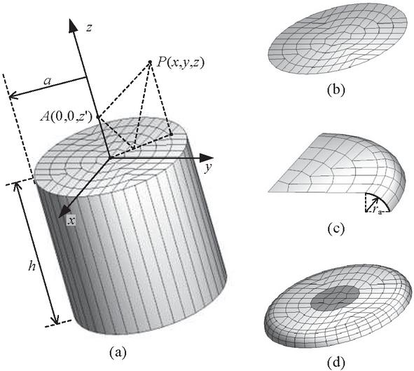
Figure 2 Different realizations of truncated ground clump. (a) Cylindrical clump. (b) Circular disk. (c) Enlarged part of disk with additional curved rim for diffraction mitigation. (d) Entire disk with a curved rim and a colored central disk, denoting part of the clump surface with local settings.

Figure 3 Examples of excitations that consist of elementary electric- and magnetic-current sources, realized as wire models. Electric-current sources are short dipoles, whereas magnetic-current sources are simulated as short square wire loops. (a) A pair of collinear electric-current and magnetic-current sources. (b) Three orthogonal electric-current sources. (c) Six coexisting sources.

To speed up the verification process, a number of equivalent wire antennas can be combined into an antenna system, as a single project, by exciting one-generator-at-a-time (OGAT) operation mode. Namely, the most consuming part in MoM/SIE simulation is the evaluation of the MoM matrix and its LU decomposition. Once the LU decomposition is performed, the solution of the matrix equations can be quickly obtained for various excitations columns by forward and backward substitution. This is exactly how the OGAT mode operates: one-by-one voltage generator is turned on, while all other generators are turned off, giving each time the corresponding excitation columns. For each excitation column, the solution is found for overall currents and electric and magnetic fields are evaluated in a grid of points of interest. If the coupling between antennas is negligible, the results obtained for each excitation column will correspond to those of a stand-alone antenna. For example, there will be no coupling at all if we combine wire antennas equivalent to vertical Hertzian electric and magnetic dipoles, as shown in Fig. 3 (a), or wire antennas equivalent to $x$ , $y$ , and $z$ -directed Hertzian electric dipole, as shown in Fig. 3 (b). Also, there is a practically negligible coupling between three orthogonal loop antennas, even if they are combined with the system of electric dipoles, resulting in configuration shown in Fig. 3 (c).

Once placed above the ground clump, all antennas will be additionally coupled. However, if the antenna system is not too close to the ground clump, this coupling remains negligible.

4 NUMERICAL EXAMPLES

In order to analyze the proposed verification procedure, we perform numerical simulations, in which SI solutions, obtained by applying the approach from [14] to equations elaborated in [31], are tested against the reference TGC MoM-based solutions. We assume an arbitrary real ground with relative permittivity $ε_{r} = 10 - j5$ and relative permeability $μ_{r} = 1$ , above which unit current sources, Hertzian dipoles, are placed and operating at frequency $f = 1$ GHz. All examples consider only the reflected field from the real ground due to the Hertzian dipoles, as well as their wire equivalents, excited by $I^{e} Δ l = 1 Am$ and $I^{m} Δ l = 1 Vm$ . The presented results are calculated in single precision. Specific to each example is the type of excitation antenna system, the type of TGC, the radius of TGC, the heights of the source $z^{'}$ and of the observation point $z$ , and the range of x- and y-coordinates for observation points.

4.1 Six-antenna scenario: Rapid verification

In the first example, the fast verification method is demonstrated. The radius of the ground clump, shown in Fig. 2 (c), and the maximum patch size are adjusted to $a = 2.5 λ$ and $d_{\max} = 0.8 λ$ , respectively. The full set of dipoles, shown in Fig. 3 (c), is placed at height $z^{'} = 0.1 λ$ . The reflected electric and magnetic fields are evaluated in yOz-plane at height of $z = z^{'}$ , in a range of y-coordinates, $y \in [0.01 λ, a]$ . The field magnitudes are shown in Fig. 4. Generally, excellent agreement between TGC and SI solutions is observed. The only exception are the results for magnetic field due to equivalent y-directed Hertzian electric dipole in a short range of y-coordinates, around $y = 0.5 λ$ , marked by a black circle in Fig. 4 (b). In this range, the magnetic field due to equivalent y-directed Hertzian electric dipole is extremely small, so that mutual coupling to equivalent Hertzian magnetic dipole antennas is not negligible. Namely, if magnetic dipoles are omitted from the scenario, which correspond to the set of dipoles shown in Fig. 3 (b), this deviation vanishes.

Figure 4 Magnitude of electric and magnetic field due to Hertzian dipoles, versus y-coordinate $(z^{'} = z = 0.1 λ, a = 2.5 λ)$ . TGC and SI solution are compared. (a) Electric field. (b) Magnetic field.

4.2 Single-antenna scenarios

In the following examples, single-antenna sources are applied, i.e. short electric dipoles (Fig. 1 (b)). The antennas are placed above the ground-clump model from Fig. 2 (d). The objective is to demonstrate the level of accuracy that can be achieved with the TGC solution. The relative error evaluated by TGC method is defined as:

δ_{X} = \frac{| X_{TGC} - X_{SI} |}{| X_{TGC} |},

(5)

where $X_{TGC}$ and $X_{SI}$ are electric or magnetic complex vector fields obtained from the TGC and SI solutions, respectively. The plots for the relative error of the magnetic field are omitted whenever they are similar to those for the electric field.

The relative error of the electric field versus x- and y-coordinates, for an x-directed Hertzian electric dipole ( $z = 0.1 λ$ , $a = 5 λ$ ) is shown in Fig. 5. The error slowly increases as we approach the rim and then rises sharply beyond it. Obviously, the error is lower in the direction that is orthogonal to the dipole axis.

In Figs. 6 (a) and 6 (b), the relative errors of the electric field due to vertical (z-oriented) and horizontal (x-directed) Hertzian electric dipole for various radii of the ground clump are presented. By increasing the radius of TGC from $a = 2.5 λ$ to $a = 10 λ$ the general level or the relative error for vertical dipole decreases from $10^{- 2}$ to 10^-3, while in the vicinity of $y = 0$ , this level is even lower by an order of magnitude. In the case of the horizontal dipole, the general level or relative error decreases from $3 \cdot 10^{- 4}$ to $3 \cdot 10^{- 5}$ . By further increase of the radius, the relative error can be lowered only if the number of unknowns is also increased and the simulation is performed in double precision.

Figure 5 Relative error of electric field due to horizontal (x-directed) Hertzian electric dipole versus x- and y-coordinates in plane $z = 0.1 λ$ ( $z^{'} = 0.1 λ, a = 5 λ$ ).

Figure 6 Relative error of electric field due to Hertzian electric dipole versus y-coordinate, for various radii, a, of the ground clump $(z^{'} = z = 0.1 λ, x = 0)$ . (a) Vertical dipole (z-directed). (b) Horizontal dipole (x-directed).

An analysis of the same scenario with the Hertzian magnetic dipoles shows that the general level of the relative error remains around $10^{- 2}$ , independently of the value of the TGC radius (first four curves in Figs. 7 (a) and 7 (b)). Obviously, an electrically small square current loop does not model the infinitesimal magnetic Hertzian dipole as well as an electrically short wire dipole models infinitesimal electric Hertzian dipole. However, by taking advantage of the duality of the expressions for fields resulting from electric and magnetic current moment above magnetic and electric grounds, respectively [31], an alternative simulation is conducted. Namely, electric dipoles are placed above lossy magnetic TGC, with converse parameters, i.e. $ε_{r} = 1$ and $μ_{r} = 10 - j5$ . The obtained electric field corresponds to the magnetic field of the original problem and vice versa. The error resulting from such dual simulation is evidently lower, as denoted by $δ_{H m}$ and given by last four curves in Figs. 7 (a) and 7 (b).

Figure 7 Relative error of electric field due to Hertzian magnetic dipole versus y-coordinates, for various radii, a, of the lossy dielectric ground clump. For comparison, results are shown for a dual problem, relative error of magnetic field due to Hertzian electric dipole above lossy magnetic ground clump $(z = 0.1 λ, x = 0, a = 5 λ)$ . (a) Vertical dipole (z-directed). (b) Horizontal dipole (x-directed).

4.3 Elevation analysis in single-antenna scenarios

Besides the size of the TGC, also the impact of the heights of the source and observation points are of interest. In that sense, a set of simulations is performed where we fix the height of the observation point and vary the height of the dipole up to 100 $λ$ , and vice versa. The relative error of the electric field due to horizontal (x-directed) Hertzian electric dipole is shown in Fig. 8.

We observe that by increasing the height of the dipole, the general level of relative error rises from $3 \cdot 10^{- 5}$ to $10^{- 2}$ , except in the vicinity of $y = 0$ , where this level is higher for half an order of magnitude (Fig. 8 (a)). In the converse case (Fig. 8 (b)), we can see that for heights of observation point up to $z = 1 λ$ , the general level of the relative error is between $3 \cdot 10^{- 5}$ and $3 \cdot 10^{- 4}$ , while by increasing this height up to $z = 100 λ$ , this level rises up to $10^{- 2}$ . This result is expected, since the high elevation above TGC reduces the model adequacy for half-space scenarios.

Figure 8 Relative error of electric field due to horizontal (x-directed) Hertzian electric dipole versus y-coordinate, for various heights of source and observation points. (a) Height variation of the source point, $z^{'}$ ( $z = 0.1 λ, x = 0, a = 5 λ$ ). (b) Height variation of the observation point, $z$ ( $z^{'} = 0.1 λ, x = 0, a = 5 λ$ ).

5 CONCLUSION

In this work, an alternative approach to verification of a family of Green’s functions, namely the homogenous half-space dyadic Green’s matrices, is presented. The elements of these matrices are typically linear combinations of numerically demanding Sommerfeld integrals and represent field responses to unit excitations, such as magnetic- or electric-current moments, i.e. elementary Hertzian dipoles.

Due to the diversity of practical half-space problems, it is often more tedious and less efficient to program a published algorithm as a reference solution for each of the possible scenarios, than to assemble a 3-D model in a proven EM tool, using basic primitives like wires, plates, and cylinders. However, testing a half-space computational procedure against complete and complex EM scenarios, e.g. by observing parameters of installed antenna, like impedance or radiation field, conceals the accuracy information on the actual algorithm that computes the elements of the Green’s matrices. Therefore, we propose verification of that numerical algorithm through simulations of fundamental scenarios that consist of elementary dipoles carefully designed as electrically small antennas, and of a model of infinite ground plane that is adjustable and thoughtfully constructed as finite-sized piece of ground, i.e. the ground clump. The procedure is easy to implement using any general-purpose 3-D EM solver in frequency domain and is applicable for all combinations of source and observation points directly above the clump, up to the height equal to the transversal dimension of the clump. With increase of the distance between the points, their heights, and the required accuracy, the resources required for the simulation also increase (e.g. number of unknowns, memory, CPU time). In order to reduce the simulation resources, the full ground-clump model is replaced by the upper boundary surface with a rounded rim (i.e. the TGC), and the number of rules is set for adjusting the simulation parameters, as well as the size and shape of antennas.

For fast and coarse verification of the DGMs, a multi-antenna scenario, based on simultaneous excitation of a set of three orthogonal electric dipoles together with a set of three orthogonal magnetic dipoles is recommended. The single-antenna scenarios allow us to attain more accurate results, where the relative error ranges from $10^{- 2}$ to $10^{- 5}$ . This is successfully demonstrated for ground clumps up to 20 $λ$ in transversal dimension. Further refinement of the finite 3-D model and of the basis functions may allow for lower error levels.

The proposed method is convenient for quick and simple verification of new algorithms that compute the elements of the half-space DGMs with somewhat limited, but controlled, accuracy. The analysis illuminates the potentials and provides guidelines for accurate verification in any 3-D EM analysis tool. Even though the given examples consider only the reflected fields, the proposed approach can also be extended to the transmitted fields, since the associated SIs are of similar nature. Naturally, care must be taken in the design of the elementary dipoles that are submerged in the ground clump.

The specific design of the TGC as open surface-of-rotation is currently limited to homogenous half-space scenarios. In future work, a multilayered TGC will be investigated and compared to the corresponding SI-based solutions.

REFERENCES

[1] A. Sommerfeld, “Über die Ausbreitung der Wellen in der drahtlosen Telegraphie,” Ann. Physik, vol. 28, pp. 665–736, 1909.

[2] A. Sommerfeld, “Über die Ausbreitung der Wellen in der drahtlosen Telegraphie,” Ann. Physik, vol. 28, pp. 665–736, 1909.

[3] H. Weyl, “Ausbreitung elektromagnetischer Wellen über einem ebenen Leiter,” Ann. Physik, vol. 60, pp. 481–500, 1919.

[4] B. Van der Pol and K. Niessen, “Über die Ausbreitung von elektromagnetischer Wellen über eine ebene Erde,” Ann. Physik, vol. 398, pp. 273–294, 1930.

[5] X. F. Li, Y. J. Xie, R. Yang, and Y. Y. Wang, “High-frequency analysis of scattering from complex targets in half space,” Applied Computational Electromagnetics Society (ACES) Journal, vol. 25, no. 5, pp. 433–443, June 2022.

[6] M. García-Fernández, G. Álvarez-Narciandi, Y. Álvarez López, and F. Las-Heras, “Array-based ground penetrating synthetic aperture radar on board an unmanned aerial vehicle for enhanced buried threats detection,” IEEE Transactions on Geoscience and Remote Sensing, vol. 61, pp. 1–18, May 2023.

[7] M. F. Pantoja, A. R. Bretones, and A. G. Yarovoy, “On the direct computation of the time-domain plane-wave reflection coefficients,” Applied Computational Electromagnetics Society (ACES) Journal, vol. 24, no. 3, pp. 294–299, June 2022.

[8] F. Rodriguez-Morales, D. Braaten, H. T. Mai, J. Paden, P. Gogineni, and J.-B. Yan, “A mobile, multichannel, UWB radar for potential ice core drill site identification in East Antarctica: Development and first results,” IEEE Journal of Selected Topics in Applied Earth Observations and Remote Sensing, vol. 13, pp. 4836–4847, Aug. 2020.

[9] B. Li, W. Ke, H. Lu, S. Zhang, and W. Tang, “Far field reconstruction based on compressive sensing with prior knowledge,” Applied Computational Electromagnetics Society (ACES) Journal, vol. 33, no. 12, pp. 1383–1389, July 2021.

[10] T. J. Cui and W. C. Chew, “Fast algorithm for electromagnetic scattering by buried 3-D dielectric objects of large size,” IEEE Transactions on Geoscience and Remote Sensing, vol. 37, no. 5, pp. 2597–2608, Sep. 1999.

[11] D. Koufogiannis, A. G. Polimeridis, M. Mattes, and J. R. Mosig, “Real axis integration of Sommerfeld integrals with error estimation,” in 2012 6th European Conference on Antennas and Propagation (EUCAP), Prague, pp. 719–723, Mar. 2012.

[12] K. Yang and A. E. Yilmaz, “A three-dimensional adaptive integral method for scattering from structures embedded in layered media,” IEEE Transactions on Geoscience and Remote Sensing, vol. 50, no. 4, pp. 1130–1139, Apr. 2012.

[13] K. A. Michalski and J. Mosig, “The Sommerfeld half-space problem revisited: From radio frequencies and Zenneck waves to visible light and fano modes,” Journal of Electromagnetic Waves and Applications, vol. 30, no. 1, pp. 1–42, 2016.

[14] N. Basta and B. Kolundžija, “Efficient evaluation of the finite part of pole-free Sommerfeld integrals in half-space problems with predefined accuracy,” IEEE Transactions on Antennas and Propagation, vol. 67, no. 7, pp. 4930–4935, July 2019.

[15] Automotive Antenna Test Solutions [Online]. Available: https://www.nsi-mi.com/applications/automotive.

[16] K. A. Michalski and J. R. Mosig, “Efficient computation of Sommerfeld integral tails – methods and algorithms,” Journal of Electromagnetic Waves and Applications, vol. 30, no. 3, pp. 281–317, 2016.

[17] V. V. Petroviæ and A. R. Djordjević, “General singularity extraction technique for reflected Sommerfeld integrals,” AEU – International Journal of Electronics and Communications, vol. 61, no. 8, pp. 504–508, 2007.

[18] M. Yuan and T. K. Sarkar, “Computation of the Sommerfeld integral tails using the matrix pencil method,” IEEE Transactions on Antennas and Propagation, vol. 54, no. 4, pp. 1358–1362, Apr. 2006.

[19] C.-P. Chang and C.-F. Yang, “A moment method solution for the shielding properties of three-dimensional objects above a lossy half space,” IEEE Transactions on Electromagnetic Compatibility, vol. 47, no. 4, pp. 723–730, Nov. 2005.

[20] W. Luo, Z. Nie, and Y. P. Chen, “Fast analysis of electromagnetic scattering from three-dimensional objects straddling the interface of a half space,” IEEE Geoscience and Remote Sensing Letters, vol. 11, no. 7, pp. 1205–1209, July 2014.

[21] X. Qi, Z. Nie, X. Que, Y. Wang, and Y. Yang, “An efficient method for analysis of EM scattering from objects straddling the interface of a half-space,” IEEE Geoscience and Remote Sensing Letters, vol. 13, no. 12, pp. 2014–2018, Dec. 2016.

[22] K. A. Michalski and J. R. Mosig, “On the complete radiation pattern of a vertical hertzian dipole above a low-loss ground,” IEEE Journal of Microwaves, vol. 1, no. 3, pp. 747–762, July 2021.

[23] J. Zhuo, F. Han, N. Liu, L. Ye, H. Liu, and Q. H. Liu, “Derivation and fast computation of dyadic Green’s functions of magnetic vector potential for unbounded uniaxial anisotropic media,” Applied Computational Electromagnetics Society (ACES) Journal, vol. 32, no. 10, pp. 862–871, July 2021.

[24] M. Kolundžija, A. R. Đorđević, and V. V. Petrović, “A new approach for accurate analysis of antennas above real ground,” in IEEE Antennas and Propagation Society International Symposium, Orlando, FL, USA, 11–16 July 1999.

[25] Ansys HFSS [Online]. Available: https://www.ansys.com/products/electronics/ansys-hfss.

[26] Altair Feko [Online]. Available: https://altair.com/feko.

[27] WIPL-D [Online]. Available: https://wipl-d.com/.

[28] J. M. Mosig and F. E. Gardiol, “Analytical and numerical techniques in the Green’s function treatment of microstrip antennas and scatterers,” IEE Proceedings H Microwaves, Optics and Antennas, vol. 130, no. 2, pp. 175–182, 1983.

[29] J. R. Mosig and A. A. Melcon, “Green’s functions in lossy layered media: integration along the imaginary axis and asymptotic behavior,” IEEE Transactions on Antennas and Propagation, vol. 51, no. 12, pp. 3200–3208, Dec. 2003.

[30] B. M. Kolundzija and N. Basta, “Method for evaluating the accuracy of Sommerfeld integrals calculations in half-space problems,” in 2023 International Conference on Electromagnetics in Advanced Applications (ICEAA), Venice, Italy, p. 435, Oct. 2023.

[31] N. Basta and B. Kolundžija, “Application of Sommerfeld-integral expressions in dielectric and magnetic half-space problems,” in 2024 11th International Conference on Electrical, Electronic and Computing Engineering (IcETRAN), Niš, Serbia, 2024.

BIOGRAPHIES

Nikola Basta was born in 1983 in Belgrade, Serbia. In 2008 he received the Dipl. Ing. degree from the School of Electrical Engineering, University of Belgrade, with a major in tele-communications. After graduation, he joined the Antenna Group at the Institute of Communications and Navigation of the German Aerospace Center (DLR), where he worked until 2014 on design and characterization of smart antennas and RF systems for GNSS application, as well as on time-domain analysis of wideband pulsed antenna arrays. Since 2014 he has been working at the School of Electrical Engineering, University of Belgrade, from which he received his Ph.D. degree in the area of computational electromagnetics. Currently, he works as assistant professor at the same school and his main interests are microwaves, applied electromagnetics, antenna systems, array signal processing and circuit theory.

Branko Kolundžija (Fellow, IEEE) was born in Zenica, Bosnia and Herzegovina, in 1958. He received the B.Sc., M.Sc., and D.Sc. degrees from the University of Belgrade, Belgrade, Serbia, in 1981, 1986, and 1990, respectively. He joined the Faculty of Electrical Engineering, University of Belgrade, in 1981, where he is currently a Full Professor in electromagnetics and antennas and propagation. He has held lectures and short courses in Ottawa, Lisbon, Urbana, Albuquerque, Syracuse, Monterrey, Stuttgart, New York, Copenhagen, Helsinki, Calgary, Zurich, Long Island, Calcutta, Tokyo, Washington, Yokohama, and Okinawa. He is the main architect of the WIPL-D software suite. He is the author or coauthor of two monographs, a chapter in a monograph, three software packages, one textbook, 32 journal articles, and 160 papers at international conferences. His research interests are numerical problems in electromagnetics, especially those applied to antennas and microwave components.