Multi-Objective Optimization of Permanent Magnet Motor Based on the Stochastic Collocation Method
Haichuan Cao, Jian Xiao, Chengzhou Yang, and Jingwei Zhu
College of Marine Electrical Engineering Dalian Maritime University, Dalian 116026, China
haichuan@dlmu.edu.cn, xj2220190706@dlmu.edu.cn, 292575223@qq.com, zjwdl@dlmu.edu.cn
Submitted On: July 20, 2025; Accepted On: December 11, 2025
ABSTRACT
In this paper, a novel multi-objective optimization method based on the stochastic collocation method (SCM) is proposed, and the effectiveness of this method is verified by finite element method (FEM) simulations on a permanent magnet synchronous motor (PMSM) with a two-layer Halbach array structure for electric vehicles (EVs). First, the proposed optimization method is introduced; then, the multi-objective optimization problem of the PMSM is defined; third, the optimization parameters are divided into two different subspaces according to their influence on the optimization objective; finally, each subspace is optimized sequentially. The FEM results show that the optimized motor has higher torque, lower torque ripple, and higher sinusoidal back-EMF.
Keywords: Design optimization, finite element method, multi-objective optimization, permanent magnet synchronous motor, stochastic collocation method, two-layer Halbach array.
1 INTRODUCTION
Electric vehicles (EVs) are powered by a battery pack and an electric motor. EVs do not produce tailpipe emissions, which helps protect the environment and improve air quality. They have become increasingly popular in recent years. Among drive motors, permanent magnet synchronous motors (PMSMs) are a promising choice because of their high energy density, high efficiency, compact size, and fast response. PMSMs are widely used for EV traction (e.g., BYD and NIO) [1, 2].
The key to improving the performance of EVs is to improve the performance of PMSMs. Research on new topologies and the optimization of design parameters are two main ways to improve the performance of the PMSMs. In recent years, many new topologies have been designed and applied to PMSMs. In [3], a consequent pole (CP) rotor topology is proposed in which the permanent magnet (PM) volume is reduced when compared with the conventional surface PMSM of EVs. Multilayer windings and non-ferromagnetic barriers are proposed to increase the torque density. In [4], a novel rotor structure with a magnetic stripe is proposed, based on the “dual stator with Halbach array” topology of the PMSM, which leads to a PMSM with greater power density. The results show that the novel rotor structure can increase the average torque. In [5], a novel interior PM rotor topology referred to here as Y-type is proposed. The new design can combine the goodness of both V- and spoke-type rotors for an FSCW stator. The goals of achieving maximum efficiency, minimum cost, and wide CPSR are accomplished in the proposed Y-type FSCW IPMSM. In [6], a novel low-cost consequent-pole permanent magnet (CPM) synchronous machine structure is proposed, considering the reluctance torque utilization. The results show that the ISCP-PMSM can obtain an almost equivalent torque and torque ripple, but with reduced PM (NdFeB) usage and cost when compared to the SPMSM.
For the optimization of design parameters, in [7], a novel automatic design method for PM motors using a Monte Carlo tree search is proposed. The optimal motor structures are determined through a tree search, in which the motors with different numbers of poles, current phase angles, PM configurations, and numbers of PMs are simultaneously considered. In [8], a robust optimization design method considering magnet material uncertainties is proposed for PM machines. The Kriging surrogate model and non-dominated sorting genetic algorithm II (NSGA-II) are adopted to solve the optimization model. In [9], a synergetic optimization approach considering both PM and armature airgap harmonics simultaneously is proposed to improve the power factor of the PM vernier machine. In [10], aiming at the uncertainty analysis method (MEAM) used in electromagnetic compatibility simulation, an uncertainty analysis method based on MEAM is proposed to test whether the uncertainty analysis method converges, and improve the efficiency and accuracy of the uncertainty analysis method. In [11], the design of experiments with the Taguchi method has been used, which is a simple and effective optimization method and requires a small number of experiments and experience. To select the best combination in multi-objective optimization, the TOPSIS method has been utilized to prioritize the optimal solutions.
Generally, motor design and optimization follow Pareto’s law, that is, the initial electromagnetic design of the motor accounts for 20% of the total time cost, and the motor parameter optimization and adjustment after the initial design account for 80%. This is because there are many design parameters of the motor, and the traditional optimization method is time-consuming; the parameters are highly nonlinear and strongly coupled. Combining individually optimized parameters does not necessarily yield a globally optimal system.
The stochastic collocation method (SCM) is a non-embedded uncertainty analysis method, which has the characteristics of high calculation accuracy and high calculation efficiency, so it is very suitable for the application of optimization design [12, 13]. Therefore, this paper selects it as an extended application of the uncertainty analysis method in optimization design and discusses its optimization performance in detail. The structure of this paper is as follows. Section 2 describes the principle of SCM. Section 3 investigates an example study for the optimization of a PMSM based on finite element method (FEM). Specific implementation and results are provided in section 4. Section 5 concludes the paper.
2 PRINCIPLE OF STOCHASTIC COLLOCATION METHOD
SCM performs uncertainty analysis without modifying the solver. It is, therefore, a non-intrusive method. The mathematical basis of this method is the Lagrange interpolation theorem.
In many practical problems, relationships between variables are not given by explicit functions and must be determined from experiments or observations. However, if a certain physical quantity in practice is observed and the corresponding observation value is obtained in several different places, interpolation technology can be used. The Lagrange interpolation method constructs a polynomial that exactly matches the observed values at the interpolation points. Such a polynomial is called a Lagrange interpolation polynomial. The specific form of one-dimensional Lagrange interpolation is:
| (1) |
where is the m-th polynomial of the independent variable x and is the function used to approximately describe ; is the -th interpolation point, while the function value is known at the interpolation point, and is:
| (2) |
For the general polynomial approximation theory, the random variable polynomial form is used to approximate the unknown FEM results. According to the Lagrange interpolation theorem, the approximate random variable polynomial can be obtained by following strategies [14]:
1. Regard the random variable as the independent variable x in equation (1);
2. Select certain points according to the random variable, which correspond to the interpolation point in equation (1);
3. When FEM simulation is carried out at these points, the simulation results can be regarded as the function value at the interpolation point in equation (1);
4. By using the Lagrange interpolation formula as shown in equation (1), a random variable polynomial can be obtained, which can be regarded as the result of FEM uncertainty analysis. The mathematical expression of the above process is:
| (3) |
where is a random variable introduced by uncertain input, and represents a random variable involving only one dimension in equation (4). is the result of uncertainty analysis in the form of polynomials of random variables, and it is the approximate function of the real result of . represents the interpolation point selected according to random variables, which is called the collocation point in SCM. represents the simulation results after a deterministic FEM simulation at the collocation point . Finally, is the Lagrange polynomial at the matching point.
Equation (4) gives the basic principle of SCM in the simulation analysis of FEM uncertainty, but only when the random variable is one-dimensional. In the case of multidimensional random variables, it is necessary to use the multidimensional Lagrange interpolation theorem. The interpolation point in the multidimensional Lagrange interpolation theorem is in the form of a tensor product in the one-dimensional case:
| (4) |
where represents the Lagrange interpolation formula at the point j in the i-th dimension, such as in equation (2), denotes the global Lagrange interpolation formula in i-th dimension, such as equation (4), and represents the number of matching points in dimension i.
Equation (2) is the calculation equation of SCM, in which the number of random variables is n and the total number of collocation points is . Based on equation (2), an FEM uncertainty analysis problem can be transformed into M deterministic FEM simulation problems, and the results of uncertainty analysis in the form of random variables are obtained.
In the optimization process, the parameters to be optimized also change within a certain range. If the range is treated as a random variable with a uniform distribution, the optimization process can be equivalent to an uncertainty analysis problem. The one-to-one correspondence between the value range and the random variable is:
| (5) |
where is the random variable obeying the uniform distribution in the range of .
According to the generalized polynomial chaos theory, SCM uses the Legendre polynomials to deal with uncertainty analysis problems with random variables of uniform distribution. The first terms of Legendre polynomials in one dimension are [15]:
| (6) |
According to the theory above, the core idea of SCM is to use the random variable polynomials to replace the FEM simulation process, and then the agent model can be sampled to obtain the uncertainty analysis results. For the optimization problem, we can also build a similar agent model and then use the exhaustive method to obtain the optimization results. As SCM has excellent computational efficiency, the establishment of the agent model only requires several forward FEM simulations, and the number of simulations is the number of collocation points. Unlike the traditional intelligent optimization algorithm, which requires repeated iterations, the proposed algorithm does not need iterations, but only a single computation; the efficiency of the proposed optimization algorithm is obviously better. However, the number of collocation points grows exponentially with the dimensionality of stochastic variables; a manifestation of the curse of dimensionality. With numerous parameters to identify, the required forward simulations increase combinatorially, thereby undermining the computational efficiency intrinsic to SCM. This inherent limitation restricts the proposed optimization framework to applications involving only a limited set of parameters. Therefore, a sensitivity analysis will be introduced in the following section to address this limitation.
3 OPTIMIZATION EXAMPLE OF A DOUBLE-LAYER HALBACH PERMANENT MAGNET ARRAY MOTOR
Figure 1 shows a brief flow chart of the application of the SCM optimization method for the double-layer Halbach PM array motor.
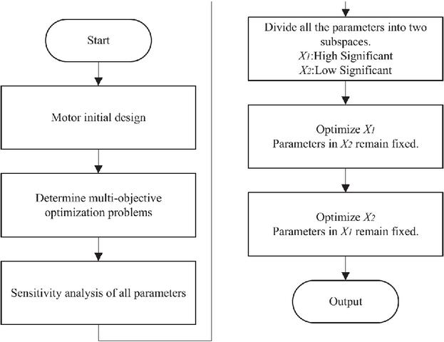
Figure 1 Flowchart of the SCM multi-objective optimization method for the Halbach motor.
Step 1: According to the practical application and design requirements of the motor, determine the initial design parameters, including structural parameters and electromagnetic parameters.
In this example, the double-layer Halbach PM array slotless motor is designed for the application of EVs. Figure 2 shows the structure of the 4-pole PM rotor with the double-layer Halbach PM array structure and the magnetization direction of the PM.
As shown in Fig. 2, the array consists of T1 (green) and T2 (purple) PMs arranged at regular intervals. The two types of PMs are magnetized in parallel, but the magnetizing direction is different. The magnetization direction of T1 PM is parallel to the radial centerline, while that of the T2 PM is perpendicular to the radial centerline. The PMs of two shapes are arranged at intervals according to the magnetizing direction in the figure to form a Halbach array. Because the magnetic fields of the PMs can be superimposed, the double-layer Halbach array is equivalent to the superposition of its upper and lower layers.
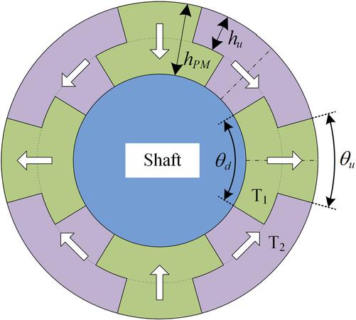
Figure 2 Rotor structure with double-layer Halbach array.
In this paper, the Halbach array near the stator is called the upper layer (subscript “u”), and the layer near the rotor shaft is called the lower layer (subscript “d”). As shown in Fig. 2, the ratio of upper and lower layer angles, and , to rotor pole angle is defined as the upper pole arc coefficient and lower-layer pole arc coefficient , respectively. Thus, the structure size of the double-layer Halbach PM array has two defined parameters: and . At the same time, for the convenience of optimization, the parameter is defined as the ratio of the thickness of the upper PM to the total PM thickness, and is defined as the tangential radius size that can be reduced by the PM. A higher value of this parameter indicates less PM material is used.
As shown in Fig. 2, the two-layer magnet structure can effectively adjust the flux distribution and reduce harmonic distortion. In our previous work [16], it was shown that if and are exchanged, remains nearly unchanged, but the fundamental flux density decreases by about 8%, which leads to a reduction of . Therefore, the optimization should be performed within the range of . The electrical parameters and initial design parameters of the motor are presented in Table 1.
Table 1 Specifications and initial design parameters of the motor
| Parameter | Description | Unit | Value |
| Rated power | kW | 4.9 | |
| n | Rated speed | r/min | 7500 |
| Rated current | A | 15 | |
| Stator outer diameter | mm | 46 | |
| Axial length | mm | 80 | |
| Number of phases | 3 | ||
| p | Number of pole pairs | 4 | |
| Upper pole arc coefficient | 0.4 | ||
| Lower pole arc coefficient | 0.6 | ||
| Air gap | mm | 1.0 | |
| Total PM thickness | mm | 11 | |
| Thickness of upper PM | mm | 6.6 | |
| Ratio of upper and total PM | 0.6 | ||
| PM of tangential reducible size | mm | 1.0 |
Table 2 Parameters to be optimized and their value range
| Parameter | Initial Value | Range |
| 0.4 | 0.30.7 | |
| 0.6 | 0.20.8 | |
| (mm) | 1.0 | 0.51.5 |
| (mm) | 11 | 1114 |
| 0.6 | 0.30.7 | |
| (mm) | 1.0 | 02 |
Step 2: Determine the SCM multi-objective optimization problem, including the determination of the parameters to be optimized, the multi-objective optimization model, and selection criteria. Selecting six of the more significant parameters according to experience as the parameters to be optimized. The selected parameters and the range to be optimized are shown in Table 2.
The optimization objectives for the motor therefore include average torque, torque ripple, and the sinusoidal quality of the back-EMF waveform. In this application, the optimization problem can be defined by:
| (7) |
where are optimization parameters, and , , and are three optimization objectives, which represent average torque, distortion rate of back-EMF waveform, and torque ripple, respectively. In the field of electric machine optimization, the weighted-sum single-objective approach is prevalent in engineering-oriented applications. In order to facilitate the selection of the optimal solution in an example, the selection criteria can be defined as:
| (8) |
where , , and are the average torque, distortion rate of the back-EMF waveform and torque ripple of the initial design, and , and are weight factors. In this example, , and are set to 0.6, 0.2, and 0.2, respectively. A single objective function can provide a fast optimization convergence process.
Step 3: Sensitivity analysis of all parameters to be optimized.
Sensitivity analysis is suitable for high-dimensional optimization problems. FEM provides high accuracy but is time-consuming. The increase of each parameter to be optimized will lead to an increase in the exponential level of FEM sampling time cost, and sensitivity analysis helps significantly reduce the computation time.
Step 4: Divide all the parameters into different subspaces.
Referring to the results of the sensitivity analysis in Step 3, input parameters are divided into two subspaces based on their influence on the output: highly significant and less significant.
Step 5: Optimize subspace .
In this step, it is determined that the parameters in subspace remain unchanged; the parameters in subspace are optimized, and the optimized parameters are passed to the next subspace.
Step 6: Optimize subspace .
Like the previous step, when optimizing subspace , ensure that the optimization results of subspace from the previous step remain unchanged, and optimize the parameters in subspace .
Step 7: Output the optimization results
The above seven steps constitute a complete optimization process. After optimization, the results can be substituted into FEM for verification, and the performance parameters before and after optimization are compared.
4 IMPLEMENTATION AND RESULTS
First, local sensitivity analysis is carried out, and all parameters are divided into two different subspaces to reduce the computational burden. Second, the proposed multi-objective optimization based on SCM is studied. Then, the accuracy of SCM is verified using FEM results. Finally, the optimal solution is compared with the initial design results, and the results are analyzed and discussed.
4.1 Sensitivity analysis
In order to reduce the computational burden, the parameters to be optimized are divided into different subspaces, and the sensitivity of the parameters is analyzed. Since the model is based on FEM, there is no clear mathematical expression between input and output, so the incremental change method is used to determine sensitivity. Because different output parameters have different units, the normalized sensitivity expression is [17]:
| (9) |
where is the sensitivity studied and is the objective function. In this paper, increment is determined to be and of the initial value, respectively.
There are six parameters to be determined with sensitivity. Each parameter requires four FEM simulations (20%, 10%, 10%, 20%). Together with the simulation of the initial parameters, a total of FEM samples are required.
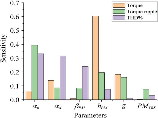
Figure 3 Local sensitivity indices of torque, distortion rate of back-EMF waveform, and torque ripple.
The results of the sensitivity analysis are shown in Fig. 3. According to the results, the parameters to be optimized are divided into two subspaces. The parameters in subspace have a significant influence on the optimization objectives, including three parameters , , and . The parameters in subspace have a less significant influence on the optimization objectives, including the remaining three parameters of , , and .
4.2 Sequential subspace optimization
According to the SCM optimization method in the second section, the sequential optimization of and subspaces is carried out, respectively. The collocation points for the and subspaces are selected in the form of a tensor product in equation (2) using the zeros of fifth-order Legendre polynomials in equation (5). These points are presented in equations (4.2) and (4.2), respectively.
| (10) | ||
| (11) |
The results of parameter identification calculated using SCM are and .
It is worth noting that, due to the introduction of sensitivity analysis, the sequential subspace optimization method is adopted and the optimization efficiency is greatly improved. For this case, the fifth-order zeros of Legendre polynomials are selected according to equation (6) and are in the form of a tensor product as shown in equation (2). In the context of finite element simulation for electrical machines, a single simulation sample requires approximately 5 minutes. If a single-level method were used to optimize all six parameters, FEM samples would be required. In contrast, the proposed sequential subspace method needs only FEM samples, reducing the number of required simulations by 98.4% and greatly improving efficiency. Meanwhile, computational time was substantially reduced from hours to hours. In addition, verification through FEM showed that the optimized parameter grouping does not affect the final trend.
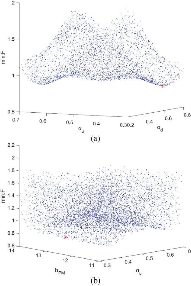
Figure 4 Relationship between objective function and optimization variables in subspace : (a) relationship between and , and (b) relationship between and , .
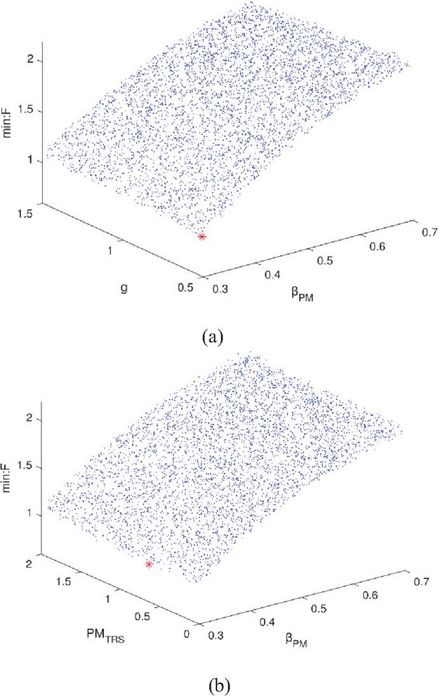
Figure 5 Relationship between objective function and optimization variables in subspace : (a) relationship between and , and (b) relationship between F and , .
Figures 4 and 5 illustrate the relationships of the objective function in equation (3) with the parameters of subspaces and , based on the SCM formulation in equation (2). The red star in Figs. 4 and 5 represents the optimization result given by SCM, which clearly verifies the effect of SCM in the area where the optimal value (i.e., the minimum value) is located.
4.3 Verification of SCM accuracy
Since optimization relies on SCM, it is necessary to verify its accuracy. SCM using equation (2) and FEM are used to sample the torque, sinusoidal distortion rate of the back-EMF waveform, and torque ripple, respectively. When optimizing , takes the initial design value. Table 3 shows the parameters obtained after the two SCM optimizations, along with the corresponding FEM results.
The initially optimized structural parameters are: . The final optimized structural parameters are: ; the average torque of the motor is 5.07 Nm, the sine wave distortion rate of back-EMF is 0.58%, and the torque ripple is 0.97%. These results yield the min .
4.4 Comparison with genetic algorithm
To verify the superiority of the proposed algorithm, it is compared with the classical Genetic Algorithm (GA). GA is a heuristic search algorithm that simulates the process of biological evolution and finds the optimal or near-optimal solution by iteratively evolving candidate solutions. In [18], the structural parameters of the motor to be optimized are first stratified based on sensitivity, and then NSGA-II is used to optimize multiple objective parameters. In [19], classical GA is used to optimize two typical electromagnetic compatibility problems, one configured with a population size of 60 for 20 iterations and the other with a population size of 60 for 10 iterations.
Table 3 Optimization results of SCM and FEM
| Parameter | Initial | ||
| Value | Optimized | Optimized | |
| 0.4 | 0.37 | 0.37 | |
| 0.6 | 0.79 | 0.79 | |
| (mm) | 11 | 12.49 | 12.49 |
| (mm) | 1 | 1 | 0.56 |
| 0.6 | 0.6 | 0.31 | |
| (mm) | 1 | 1 | 0.39 |
| FEM | |||
| (Nm) | 4.47 | 4.78 | 5.07 |
| 1.11 | 1.22 | 0.58 | |
| 1.26 | 1.11 | 0.97 | |
| min | |||
| 1 | 0.95709 | 0.78746 | |
In this paper, three objective functions have been combined into one F function; therefore, classical GA is chosen. First, the pre-experiment is configured with a population size of 80 and conducted through 12 iterations. The results are shown in Table 4.
Table 4 Optimization results of GA (80-12)
| Iteration times | Simulation times | min F |
| 1 | 160 | 1 |
| 2 | 240 | 0.99353 |
| 3 | 320 | 0.99203 |
| 4 | 400 | 0.96367 |
| 5 | 480 | 0.93284 |
| 6 | 560 | 0.92226 |
| 7 | 640 | 0.90597 |
| 8 | 720 | 0.83544 |
| 9 | 800 | 0.78753 |
| 10 | 880 | 0.77665 |
| 11 | 960 | 0.77665 |
| 12 | 1040 | 0.77665 |
In addition to the GA configuration with a population size of 80 and 12 iterations (used for preliminary comparison in this study), we also tested a more common configuration with a population size of 30 and 20 iterations, as suggested in the literature. The results are shown in Table 5.
The crossover probability and mutation probability of the two sets of genetic algorithms are set to be the same, namely and . The finally converged simulation results are: the average torque of the motor is 5.07 Nm, the sine wave distortion rate of back-EMF is 0.52%, and the torque ripple is 0.97%. These results make min .
Finally, for reference, the optimized result for the composite objective function using SCM methodology was 0.78746. For comparison, as can be seen from Table 4, the GA with a population size of 80 and 12 iterations reached a value of 0.78753 for the objective function by the 9th generation. From Table 5, it is observed that the GA with a population size of 30 and 20 iterations achieved a slightly higher value of 0.78768 for by the 18th generation. Under the same parameters, compared to the latter, the former can converge more quickly due to having more samples. Thus, the GA requires 6301040 FEM runs, which is much larger than the SCM’s 250 runs.
Both GA cases confirm that SCM achieves comparable accuracy with far fewer FEM evaluations, while the GA needs many more iterations to converge.
Table 5 Optimization results of GA (30-20)
| Iteration times | Simulation times | min |
| 1 | 60 | 1 |
| 2 | 90 | 0.99703 |
| 3 | 120 | 0.99190 |
| 4 | 150 | 0.96867 |
| 5 | 180 | 0.96303 |
| 6 | 210 | 0.95720 |
| 7 | 240 | 0.95139 |
| 8 | 270 | 0.93949 |
| 9 | 300 | 0.93201 |
| 10 | 330 | 0.92726 |
| 11 | 360 | 0.91097 |
| 12 | 390 | 0.90336 |
| 13 | 420 | 0.86479 |
| 14 | 450 | 0.86267 |
| 15 | 480 | 0.84044 |
| 16 | 510 | 0.83531 |
| 17 | 540 | 0.81726 |
| 18 | 570 | 0.78768 |
| 19 | 600 | 0.77665 |
| 20 | 630 | 0.77665 |
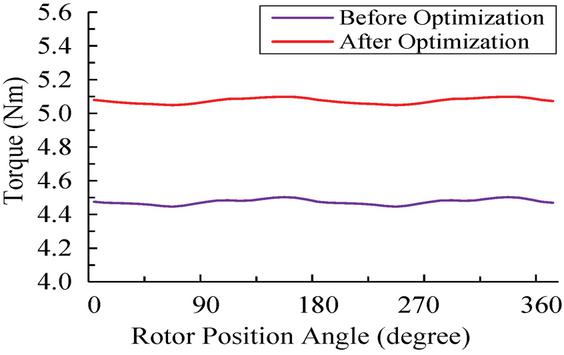
Figure 6 Comparison of torque before and after optimization.
4.5 Results comparison
After validating the SCM model, the optimal solution in Figs. 4 and 5 is credible. Figures 6 and 7 show comparisons of torque and back-EMF waveforms between the optimal solution and the initial design, respectively, and a detailed numerical comparison is shown in Table 3. In the initial design, the average torque of the motor is 4.47 Nm, the sine wave distortion rate of back-EMF is 1.11%, and the torque ripple is 1.26%. After optimization by the SCM method, the average torque reaches 5.07 Nm, the sine wave distortion rate of back-EMF is 0.58%, and the torque ripple is 0.97%. It can be seen that the motor optimized by SCM not only achieves higher torque and lower torque ripple but also improves the sinusoidal quality of back-EMF.
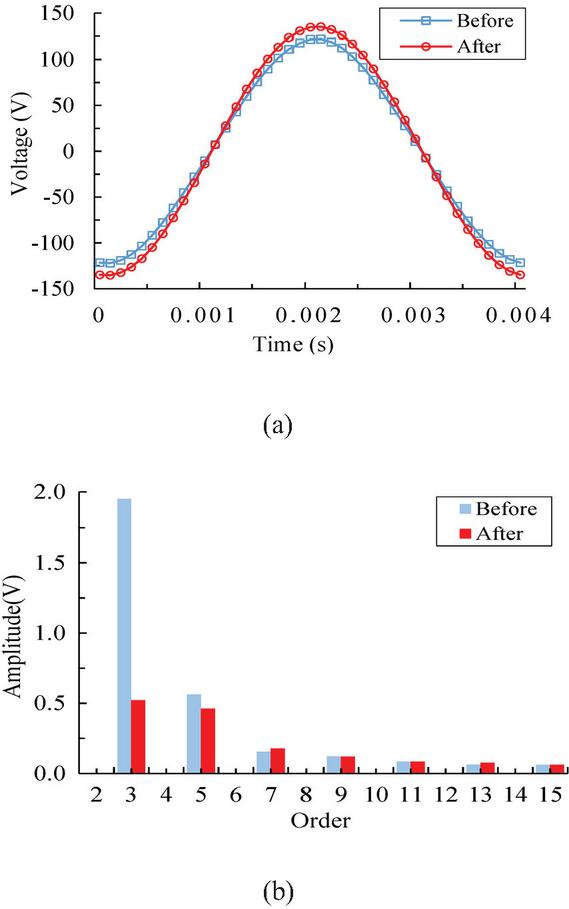
Figure 7 Comparison of back-EMF and harmonic waveform before and after optimization: (a) back-EMF and (b) harmonic wave.
5 CONCLUSION
This paper proposes a multi-objective optimization algorithm based on SCM to achieve an efficient structural design of PM motors. A double-layer Halbach PM motor is used as an example, with torque, back-EMF, THD, and torque ripple as optimization objectives. The design parameters are divided into two subspaces through sensitivity analysis and optimized separately under the SCM framework to improve efficiency and reduce computation. Compared with GA, FEM-based results show that SCM provides clear advantages in optimization efficiency.
ACKNOWLEDGMENT
This research was funded by the National Natural Science Foundation of China under grant number 52377037.
REFERENCES
[1] T. A. Huynh and M. F. Hsieh, “Performance analysis of permanent magnet motors for electric vehicles (EV) traction considering driving cycles,” Energies, vol. 11, no. 6, p. 1385, May 2018.
[2] C. Gong, Y. Hu, J. Gao, Z. Wu, J. Liu, H. Wen, and Z. Wang, “Winding-based DC-bus capacitor discharge technique selection principles based on parametric analysis for EV-PMSM drives in post-crash conditions,” IEEE Transactions on Power Electronics, vol. 36, no. 3, pp. 3551–3562, Mar. 2021.
[3] H. Dhulipati, S. Mukundan, Z. Li, E. Ghosh, J. Tjong, and N. C. Kar, “Torque performance enhancement in consequent pole PMSM based on magnet pole shape optimization for direct-drive EV,” IEEE Transactions on Magnetics, vol. 57, no. 2, pp. 1–7, Feb. 2021.
[4] W. Wei, J. Zhang, J. Yao, S. Tang, and S. Zhang, “Performance analysis and optimization of power density enhanced PMSM with magnetic stripe on rotor,” Energies, vol. 13, no. 17, p. 4457, Sep. 2020.
[5] R. Dutta, A. Pouramin, and M. F. Rahman, “A novel rotor topology for High-Performance fractional slot concentrated winding interior permanent magnet machine,” IEEE Transactions on Energy Conversion, vol. 36, no. 2, pp. 658–670, June 2021.
[6] W. Chai, Z. Cai, B. I. Kwon, and J. W. Kwon, “Design of a novel low-cost consequent-pole permanent magnet synchronous machine,” IEEE Access, vol. 8, pp. 194251–194259, 2020.
[7] H. Sato and H. Igarashi, “Automatic design of PM motor using Monte Carlo tree search in conjunction with topology optimization,” IEEE Transactions on Magnetics, vol. 58, no. 9, pp. 1–4, Sep. 2022.
[8] J. Wu, X. Zhu, D. Fan, Z. Xiang, L. Xu, and L. Quan, “Robust optimization design for permanent magnet machine considering magnet material uncertainties,” IEEE Transactions on Magnetics, vol. 58, no. 2, pp. 1–7, Feb. 2022.
[9] L. Xu, W. Wu, and W. Zhao, “Airgap magnetic field harmonic synergetic optimization approach for power factor improvement of PM vernier machines,” IEEE Transactions on Industrial Electronics, vol. 69, no. 12, pp. 12281–12291, Dec. 2022.
[10] J. Bai, L. Wang, D. Wang, A. P. Duffy, and G. Zhang, “Validity evaluation of the uncertain EMC simulation results,” IEEE Transactions on Electromagnetic Compatibility, vol. 59, no. 3, pp. 797–804, June 2017.
[11] M. Naseh, S. Hasanzadeh, S. M. Dehghan, H. Rezaei, and A. S. Al-Sumaiti, “Optimized design of rotor barriers in PM-assisted synchronous reluctance machines with Taguchi method,” IEEE Access, vol. 10, pp. 38165–38173, 2022.
[12] J. Bai, G. Zhang, A. P. Duffy, and L. Wang, “Dimension-reduced sparse grid strategy for a stochastic collocation method in EMC software,” IEEE Transactions on Electromagnetic Compatibility, vol. 60, no. 1, pp. 218–224, Feb. 2018.
[13] J. Bai, K. Gou, J. Sun, and N. Wang, “Application of the multi-element grid in EMC uncertainty simulation,” Appl. Comput. Electromagn. Soc. J., vol. 37, no. 4, pp. 428–434, Apr. 2022.
[14] Y. M. You, “Optimal design of PMSM based on automated finite element analysis and metamodeling,” Energies, vol. 12, no. 24, p. 4673, Dec. 2019.
[15] D. Xiu and G. Karniadakis, “The Wiener-Askey polynomial chaos for stochastic differential equations,” SIAM Journal on Scientific Computing, vol. 24, no. 2, pp. 619–644, Oct. 2002.
[16] B. Kou, H. Cao, W. Li, and X. Zhang, “Analytical analysis of a novel double layer Halbach permanent magnet array,” Transactions of China Electrotechnical Society, vol. 30, no. 10, pp. -76, 2015.
[17] J. Morio, “Global and local sensitivity analysis methods for a physical system,” European Journal of Physics, vol. 32, no. 6, pp. 1577–1583, Nov. 2011.
[18] W. Yan, H. Chen, H. Liu, X. Ma, Z. Lv, X. Wang, R. Palka, L. Chen, and K. Wang “Design and multi-objective optimization of switched reluctance machine with iron loss,” IET Electr. Power Appl., vol. 13, no. 4, pp. 435–444, Apr. 2019.
[19] X. Niu, S. Liu, and R. Qiu, “Efficient electromagnetic compatibility optimization design based on the stochastic collocation method,” Appl. Comput. Electromagn. Soc. J., vol. 39, no. 6, pp. 533–541, June 2024.
BIOGRAPHIES

Haichuan Cao was born in China and is a Ph.D. lecturer. His current research interests are permanent magnet motors, marine rim propulsion motors and related fields. His main research areas are motor structure design and optimization, motor magnetic field analysis and optimization calculation, and drive and control technology.

Jian Xiao received the bachelor’s degree in engineering. In 2023, he graduated from Dalian Maritime University, majoring in marine electronics and electrical engineering. He is currently a graduate student in electrical engineering at Dalian Maritime University, and his main research direction is the design and optimization analysis of six-phase permanent magnet linear motors.

Chengzhou Yang was born in 1996. He completed a master’s degree in Electrical Engineering at Dalian Maritime University from 2020 to 2023, with research specializing in the design and optimization of switched reluctance motors. Since 2023, he has been employed at State Grid Shandong Electric Power Company Laiwu Power Supply Company.

Jingwei Zhu (Member, IEEE) received the B.S. degree in automation instrumentation engineering from Jinzhou Institute of Technology, Jinzhou, China, in 1985, the M.S. degree in electronic engineering from the Shenyang University of Technology, Shenyang, in 1990, and the Ph.D. degree in electrical engineering from Adelaide University, Adelaide, SA, Australia, in 2008. He was a Lecturer and an Associate Professor with the Jinzhou Institute of Technology, from 1985 to 1999. In 2000, he joined the Marine Electrical Engineering College, Dalian Maritime University, Dalian, where he is currently a Professor. His research interests include design and control for electrical machine systems, power electronic devices, and sustainable energy generation.
ACES JOURNAL, Vol. 40, No. 12, 1226–1235
DOI: 10.13052/2025.ACES.J.401210
© 2026 River Publishers