Quantitative Analysis of Confidence Interval for Electromagnetic Characteristics of Hypersonic Targets

Yupeng Zhu¹, Dina Chen², Huaguang Bao², and Min Han^1,*

¹Institute of Systems Engineering Academy of Military Sciences, People’s Liberation Army of China, Beijing 100082, China
nudtyp@163.com, hanminchina@163.com
^∗Corresponding Author

²Nanjing University of Science and Technology Nanjing 210094, China
1390737464@qq.com, hgbao@njust.edu.cn

Submitted On: July 29, 2025 Accepted On: October 07, 2025

Abstract

In response to the current lack of rapid and efficient techniques for uncertainty analysis in electromagnetic problems, this paper proposes an efficient uncertainty quantification method based on the finite-difference time-domain (FDTD) method. A conformal FDTD formulation integrated with polynomial chaos expansion (PCE) is comprehensively derived. For random input variables exhibiting Gaussian distribution characteristics, Hermite polynomial expansion and Galerkin testing are employed. Furthermore, by incorporating the Runge-Kutta time-stepping scheme, the method efficiently quantifies electromagnetic scattering characteristics considering stochastic variations in plasma electron density of hypersonic targets. Numerical experiments demonstrate that the proposed approach provides a reliable framework for uncertainty analysis in complex electromagnetic environments.

Keywords: Electromagnetic characteristics, hypersonic target, polynomial chaos expansion, uncertainty..

1 INTRODUCTION

Near-space refers to the region between 20 km and 100 km altitude, which includes most of the stratosphere, the entire mesosphere, and parts of the thermosphere. When hypersonic targets reach near-space regions during high-speed flight, they encounter a highly complex high-temperature plasma sheath [1]. As radio signals propagate through the plasma sheath, they experience absorption and scattering effects that alter the electromagnetic characteristics of the vehicle, posing significant challenges for communication and radar detection of hypersonic vehicles [2, 3]. The hypersonic flow environment is further complicated by high-temperature non-equilibrium flows, chemical reactions, and thermodynamic non-equilibrium. Regarding confidence intervals in radar detection, the primary question is it the target or just noise. The decision is based on comparing the received signal power to a threshold. The significance of confidence intervals in radar tracking is accurate estimation of the tracked motion state of the target. Although environmental parameters can be measured on the ground, it is prohibitively expensive. Thus, numerical simulation techniques are crucial for analyzing the electromagnetic properties of hypersonic targets [4, 5]. Despite the high accuracy of numerical methods, real-world problems often introduce numerous uncertainty factors. This has led to a strong interest in studying the effects of these stochastic fluctuations to enhance the precision and reliability of engineering analyses.

Considering the actual environment, manufacturing processes, and other factors, practical electromagnetic systems are susceptible to uncertainties such as electromagnetic interference (EMI) and electromagnetic compatibility (EMC) [6, 7, 8]. It is crucial to consider and quantify the impact of these uncertainties through methods like electromagnetic compatibility analysis and bioelectromagnetic analysis [9]. There are primarily two types of numerical quantification methods. One type is statistical methods based on sampling theory, with the most famous being the Monte Carlo (MC) method [10]. Hastings et al. used the MC-FDTD method to analyze the electromagnetic scattering characteristics of random rough surfaces [11]. While the Monte Carlo method is simple to implement, it suffers from low convergence rates, resulting in significant computational time. The other type is stochastic methods based on probability theory, which include several techniques. Smith proposed the Stochastic FDTD (SFDTD) method using Taylor series expansion and applied it to bioelectromagnetic simulations, achieving an analysis of the electromagnetic properties of multilayer skin tissues considering uncertainties in dielectric parameters and conductivity [12, 13, 14]. Nguyen et al. employed the SFDTD method to study the electromagnetic characteristics of magnetized plasma with random electron and ion concentrations in the atmosphere [15]. Silly-Carette et al. used the Stochastic Collocation (SC) method, combined with FDTD simulation, to analyze the uncertainty of the impact of plane waves with random incident angles on human head radiation [16]. Edwards et al. combined the PCE technique with the FDTD method to analyze EMC problems, quantifying uncertainties in scenarios involving uniformly distributed reflection coefficients of shielding plates and the random variation of dielectric sphere radii, dielectric parameters, and magnetic permeability [17]. Austin and Sarris utilized the FDTD method based on PCE technology to conduct efficient analysis of integrated circuits with geometrically varying dimensions [18]. Pyrialakos et al. used the FDTD method, based on PCE technology and the Karhunen-Loeve (KL) expansion method, for spatially inhomogeneous materials with stochastic exponential gradients. This allowed for rapid analysis of the electromagnetic characteristics of uncertain problems by decoupling multi-input variable random processes and reducing the polynomial order describing random output variables [19]. Lin et al. proposed a framework for uncertainty quantification based on the isogeometric boundary element method and PCE method in the acoustic field and robust shape optimization for sound barriers [20]. Jiang et al. proposed a novel and comprehensive computational framework based on intrusive polynomial chaos approach to effectively analyze the uncertainty problem of thermomagnetic convection caused by random temperature fluctuations [21]. In comparison to Monte Carlo methods, probabilistic-based stochastic methods are operationally intricate but exhibit enhanced convergence characteristics.

Yang et al. introduced the Monte Carlo method to streamline the uncertainty analysis in the measurement of electromagnetic parameters for absorbing materials using the transmission/reflection method and investigated the key factors influencing system uncertainty [22]. In electromagnetic compatibility analysis, the quantification of uncertainty frequently encounters challenges caused by the curse of dimensionality, Jiang et al. proposes an enhanced sparse polynomial chaos expansion method that combines hyperbolic truncation, E-optimality criterion, and the subspace pursuit algorithm to improve both computational efficiency and model accuracy [23].

Given the absence of fast and efficient analysis techniques for uncertain electromagnetic problems in the time-domain differential equation method, this paper explores an efficient uncertainty analysis technique based on the time-domain differential equation method. Specifically, we investigate the conformal finite-difference time-domain (FDTD) method augmented with polynomial chaos expansion (PCE) technology. In this study, we focus on employing the Hermite polynomial expansion and Galerkin test to address random problems characterized by Gaussian distribution of input variables. Additionally, we integrate the Runge-Kutta exponential time-history difference technique into the analysis. Through these combined approaches, we achieve quantitative analysis of the uncertain electromagnetic scattering characteristics of hypersonic target plasma, specifically considering the random variation of electron concentration. The proposed methodology allows for a thorough examination of the uncertainties associated with the scattering behavior of hypersonic target plasma. By effectively incorporating the PCE technology and specialized numerical techniques within the conformal FDTD framework, we can analyze the electromagnetic response of the system in the presence of random variations in electron concentration. This research significantly contributes to advancing our understanding of the uncertain electromagnetic properties of hypersonic targets, enabling more accurate characterization and prediction of their scattering characteristics.

2 POLYNOMIAL CHAOS EXPANSION TECHNIQUES

The Monte Carlo method is a classical sampling statistical method that offers clear principles and easy implementation. However, it is often time-consuming due to the need for repeated sampling calculations. In contrast, PCE technology, as a probabilistic statistical method, conducts an orthogonal polynomial expansion on random input variables and their corresponding response variables. This approach transforms uncertainty quantification into solving expansion coefficients, allowing us to obtain statistical characteristics of uncertainty problems through a single simulation. In deterministic time-domain electromagnetic simulations, the computational dimension typically consists of the time dimension (t) and spatial dimensions (x, y, z). When uncertain variables are present in the electromagnetic system, an additional dimension $\xi$ is introduced to capture the randomness of electromagnetic waves. For conventional time-domain differential equation methods, basis functions or direct difference methods are employed for spatial expansions, while difference methods are used for time expansions. Therefore, when dealing with the newly introduced dimension, suitable methods must be employed for expansion. In this paper, we adopt the polynomial chaos expansion method on the additional dimension. This involves using orthogonal polynomials to expand random variables. The selection of orthogonal polynomials should consider the probabilistic statistical distribution of the random input variables. If the random input variable follows a Gaussian probability distribution, Hermite polynomials can be chosen. If the random input variables follow a uniform distribution, Legendre polynomials can be selected. These choices are made based on the statistical properties of the random variables to ensure accurate representation and analysis of the uncertainties in the electromagnetic system.

2.1 Gaussian probability distribution

Assuming that the random input variable $In(\xi )$ satisfies the Gaussian probability distribution, then the input variable can be described as:

$$In(\xi )={\mu }_{In}+{\sigma }_{In}\xi .$$

(1)

Here ${\mu }_{In}$ is the average value,${\sigma }_{In}$ is the standard deviation, and $\xi$ is a random quantity satisfying the standard normal distribution. Using Hermite polynomial to expand the uncertain response variable $f(r,t,\xi )$:

$$f(r,t,\xi )=\sum _{k=0}^{k=p}{\psi }_k(\xi )f^k(r,t).$$

(2)

Here ${\psi }_k(\xi )$ is Hermite polynomial and $p$ is polynomial order. The Hermite polynomial of order $k$ is defined as:

$${\psi }_k(\xi )={(-1)}^k{e}^{{\xi }^2/2}\frac{d^k}{d{\xi }^k}{e}^{-{\xi }^2/2}.$$

(3)

Hermite polynomials satisfy the following recursion relation and orthogonality:

$${\psi }_0(\xi )=1,{\psi }_1(\xi )=\xi ,$$
$${\psi }_{k+1}(\xi )=\xi {\psi }_k(\xi )-k{\psi }_{k-1}(\xi ),k>1,$$	(4)
$$⟨{\psi }_m(\xi ),{\psi }_n(\xi )⟩={\int }_{-\mathrm{\infty }}^{+\mathrm{\infty }}{\psi }_m(\xi ){\psi }_n(\xi )e^{-{\xi }^2/2}\mathit{d}\xi$$
$$=n!\sqrt{2\pi }{\delta }_{mn}.$$	(5)

Here ${\delta }_{mn}$ is the Kronecker impulse function.

2.2 Uniform distribution

If the random input variable $In(\xi )$ follows the uniform distribution of [a,b], then the input variable can be described as:

$$In(\xi )=\frac{b-a}{2}\xi +\frac{a+b}{2}.$$

(6)

Here $\xi$ follows the uniform distribution of $[-1,1]$. The Legendre polynomial is used to expand the uncertain response variable $f(r,t,\xi )$:

$$f(r,t,\xi )=\sum _{k=0}^{k=p}{P}_k(\xi )f^k(r,t).$$

(7)

Here $P_k(\xi )$ represents the Legendre polynomial and $p$ is the polynomial order. The Hermite polynomial of order $k$ is defined as:

$$P_k(\xi )=\frac{1}{2^{k}k!}\frac{d^k}{d{\xi }^k}[{({\xi }^2-1)}^k].$$

(8)

The Legendre polynomial satisfies the following recursion relation and orthogonality:

$$P_0(\xi )=1,P_1(\xi )=\xi ,$$
$$(k+1)P_{k+1}(\xi )=(2k+1)\xi P_k(\xi )-k{P}_{k-1}(\xi ),k>1,$$	(9)
$$⟨P_m(\xi ),P_n(\xi )⟩={\int }_{-1}^1{P}_m(\xi )P_n(\xi )\mathit{d}\xi =\frac{2}{2n+1}{\delta }_{mn}.$$	(10)

3 UNCERTAINTY ELECTROMAGNETIC ANALYSIS

Plasma is a unique state of matter consisting of ions, electrons, and non-ionized neutral particles. It is characterized by its collective behavior and is primarily influenced by electromagnetic forces. Plasma exists in a neutral state overall, despite the presence of charged particles. Plasma finds a wide range of applications across various fields, including biomedical, electronic, and military domains. In the realm of electronics, plasma is utilized in microelectronics for processes like plasma etching and deposition, which are crucial in the fabrication of integrated circuits and other electronic devices. Plasma displays, such as plasma TVs, rely on the ionization of gas to produce light. High-power microwave devices also employ plasma to generate and control electromagnetic radiation. Plasma-based techniques can be used to reduce radar cross-section and improve the stealth capabilities of military equipment. Additionally, plasmas can be harnessed to enhance the aerodynamic properties of aircraft by controlling the boundary layer flow around the surface. The electromagnetic analysis of plasma needs to correctly extract the equivalent electromagnetic parameters of plasma, where plasma frequency ${\omega }_p$ and plasma collision frequency $v_c$ are the two main parameters.

The oscillation frequency of electrons and ions in plasma under the combined action of external disturbance and coulomb force is called the oscillation angular frequency of plasma, also known as the cut-off frequency of plasma. The plasma frequency ${\omega }_p$ is the sum of the angular frequency of electron oscillation ${\omega }_{pe}$ and the angular frequency of ion oscillation ${\omega }_{pi}$, namely ${\omega }_p={\omega }_{pe}+{\omega }_{pi}$. The angular frequency of electron oscillation and the angular frequency of ion oscillation have the following forms:

$${\omega }_{pe}=\sqrt{\frac{n_e{q}_e^2}{m_e{\epsilon }_0}},{\omega }_{pi}=\sqrt{\frac{n_i{q}_e^2}{m_i{\epsilon }_0}},$$

(11)

where $n_e$ is the number of electrons per unit volume, $n_i$ is the number of ions per unit volume, $q_e$ is the electron charge, $m_e$ is the electron mass, $m_i$ is the ion mass, and ${\epsilon }_0$ is the dielectric constant of free space. Under normal aerodynamic conditions, $m_i$ is much greater than $m_e$. Correspondingly, ${\omega }_{pi}$ is much smaller than ${\omega }_{pe}$. The angular frequency of ion oscillation is negligible, so it can be approximated ${\omega }_p\approx {\omega }_{pe}$. The angular frequency of plasma oscillation is expressed as:

$${\omega }_p\approx \sqrt{\frac{n_e{q}_e^2}{m_e{\epsilon }_0}}.$$

(12)

Plasma collision frequency $v_c$ is also a necessary parameter in the dielectric constant of the plasma, in which the electron collision frequency dominates. There are many kinds of collisions between particles in plasma, the most important part is the collision between electrons and ions and the collision between electrons and neutral particles.

The collision frequency between electrons and neutral particles is:

$$v_{em}=6.3\times {10}^{-9}{n}_m\sqrt{\frac{T}{300}}.$$

(13)

The collision frequency of electrons and ions is:

$$v_{ei}=\frac{5.5n_i}{T_e^{3/2}}\left[\ln \left(\frac{280T_e}{n_i^{1/3}}\right)+\frac{1}{3}\ln \left(\frac{T}{T_e}\right)\right].$$

(14)

Normally,$v_{em}\gg v_{ei}$. Therefore, it can be approximated $v_c\approx v_{em}$. The expression of plasma collision frequency is:

$$v_c\approx v_{em}=6.3\times {10}^{-9}{n}_m\sqrt{\frac{T}{300}},$$

(15)

where $n_m$ is the density of neutral particles in the gas.

The electromagnetic parameters of unmagnetized plasma can be described by the Drude model in the following form:

$$\epsilon ={\epsilon }_0\left(1+\frac{{\omega }_p^2}{j\omega (j\omega +v_c)}\right).$$

(16)

Substituting the above equation into the frequency-domain Maxwell curl equations, we get:

$$j\omega {\epsilon }_0\left(1+\frac{{\omega }_p^2}{j\omega (j\omega +v_c)}\right)\mathit{E}=\nabla \times \mathit{H},$$	(17)
$$j\omega \mu \mathit{H}=-\nabla \times \mathit{E}.$$	(18)

By introducing the polarization current density $\mathit{J}$ and converting the above equation into the time-domain, the following expression can be obtained:

$${\epsilon }_0\frac{\partial \mathit{E}}{\partial t}+\mathit{J}=\nabla \times \mathit{H}.$$	(19)
$$\mu \frac{\partial \mathit{H}}{\partial t}=-\nabla \times \mathit{E}.$$	(20)
$$\frac{\partial \mathit{J}}{\partial t}+v_c\mathit{J}={\epsilon }_0{\omega }_p^2\mathit{E}.$$	(21)

In a rectangular coordinate system, the component of polarization current density in the $\frac{d{J}_x}{dt}+v{J}_x={\epsilon }_0{\omega }_p^2{E}_x$ direction is expressed as:

$$\frac{\partial {\mathit{J}}_x}{\partial t}+v_c{\mathit{J}}_x={\epsilon }_0{\omega }_p^2{\mathit{E}}_x.$$

(22)

We multiply both sides of equation (22) by the factor $e^{v_{c}t}$ and simplify to get:

$$\frac{\partial ({\mathit{J}}_x{e}^{v_{c}t})}{\partial t}={\epsilon }_0{\omega }_p^2{\mathit{E}}_x.$$

(23)

Using second-order Runge-Kutta time difference and simplifying the above equation, the following recurrence relationship can be obtained:

$J_x^{n+1}$	$=e^{-{\nu }_c\mathrm{\Delta }t}{J}_x^n+{\displaystyle \frac{1-e^{-{\nu }_c\mathrm{\Delta }t}}{{\nu }_c}}{\epsilon }_0{\omega }_p^2{E}_x^n$
	$+{\displaystyle \frac{(e^{-{\nu }_c\mathrm{\Delta }t}-1+{\nu }_c\mathrm{\Delta }t)}{{\nu }_c^2\mathrm{\Delta }t}}[{\epsilon }_0{\omega }_p^2{E}_x^{n+1}-{\epsilon }_0{\omega }_p^2{E}_x^n].$	(24)

Equation (19) can be discretized by using central difference in time as:

$$E_x^{n+1}=E_x^n+\frac{\mathrm{\Delta }t}{{\epsilon }_0}{(\nabla \times \mathit{H})}_x-\frac{\mathrm{\Delta }t}{2{\epsilon }_0}(J_x^{n+1}+J_x^n).$$

(25)

By substituting equation (24) into equation (25) and simplifying, we get:

$E_x^{n+1}$	$={\displaystyle \frac{1}{1+\frac{{\omega }_p^2}{2{\nu }_c^2}(e^{-{\nu }_c\mathrm{\Delta }t}-1+{\nu }_c\mathrm{\Delta }t)}}$
	$\times \{[1-{\displaystyle \frac{\mathrm{\Delta }t{\omega }_p^2}{2{\nu }_c}}(1-e^{-{\nu }_c\mathrm{\Delta }t})$
	$+{\displaystyle \frac{{\omega }_p^2}{2{\nu }_c^2}}(e^{-{\nu }_c\mathrm{\Delta }t}-1+{\nu }_c\mathrm{\Delta }t)]E{}_x{}^n$
	$+{\displaystyle \frac{\mathrm{\Delta }t}{{\epsilon }_0}}{(\nabla \times \mathit{H})}_x-{\displaystyle \frac{\mathrm{\Delta }t}{2{\epsilon }_0}}(1+e^{-{\nu }_c\mathrm{\Delta }t})J_i^n\}.$	(26)

Similar treatment is done in the other directions, and the iterative formula of the magnetic field is the same as that of the ordinary FDTD, which means that the plasma can still be treated with traditional metal conformal treatment when it is located at the metal interface. From equations (24) and (3), the iterative formula of Runge-Kutta in the discretized three-dimensional unmagnetized plasma can be obtained. The following is a concrete expression for $J_x$ and $E_x$ in the $x$ direction at the coordinates $(i+1/2,j,k)$. The form of the $y$ and $z$ direction components is similar, so those expressions are omitted.

$J_x^n(i+{\displaystyle \frac{1}{2}},j,k)$
$=e^{-{\nu }_c\mathrm{\Delta }t}{J}_x^{n-1}(i+{\displaystyle \frac{1}{2}},j,k)$
$+{\displaystyle \frac{1-e^{-{\nu }_c\mathrm{\Delta }t}}{{\nu }_c}}{\epsilon }_0{\omega }_p^2{E}_x^{n-1}(i+{\displaystyle \frac{1}{2}},j,k)$
$+{\displaystyle \frac{(e^{-{\nu }_c\mathrm{\Delta }t}-1+\nu \mathrm{\Delta }t)}{{\nu }_c^2\mathrm{\Delta }t}}$
$\times [{\epsilon }_0{\omega }_p^2{E}_x^n(i+{\displaystyle \frac{1}{2}},j,k)$
$-{\epsilon }_0{\omega }_p^2{E}_x^{n-1}(i+{\displaystyle \frac{1}{2}},j,k)].$	(27)
$E_x^{n+1}(i+{\displaystyle \frac{1}{2}},j,k)$
$={\displaystyle \frac{1}{1+\frac{{\omega }_p^2}{2{\nu }_c^2}(e^{-{\nu }_c\mathrm{\Delta }t}-1+{\nu }_c\mathrm{\Delta }t)}}$
$\times \{[1-{\displaystyle \frac{\mathrm{\Delta }t{\omega }_p^2}{2{\nu }_c}}(1-e^{-{\nu }_c\mathrm{\Delta }t})$
$+{\displaystyle \frac{{\omega }_p^2}{2{\nu }_c^2}}(e^{-\nu \mathrm{\Delta }t}-1+{\nu }_c\mathrm{\Delta }t)]$
$\times E_x^n(i+{\displaystyle \frac{1}{2}},j,k)$
$+{\displaystyle \frac{\mathrm{\Delta }t}{{\epsilon }_0}}[{\displaystyle \frac{1}{\mathrm{\Delta }y}}(H_z^{n+1/2}(i+{\displaystyle \frac{1}{2}},j+{\displaystyle \frac{1}{2}},k)$
$-H_z^{n+1/2}(i+{\displaystyle \frac{1}{2}},j-{\displaystyle \frac{1}{2}},k))$
$-{\displaystyle \frac{1}{\mathrm{\Delta }z}}(H_y^{n+1/2}(i+{\displaystyle \frac{1}{2}},j,k+{\displaystyle \frac{1}{2}})$
$-H_y^{n+1/2}(i+{\displaystyle \frac{1}{2}},j,k-{\displaystyle \frac{1}{2}}))]$
$-{\displaystyle \frac{\mathrm{\Delta }t}{2{\epsilon }_0}}(1+e^{-{\nu }_c\mathrm{\Delta }t})J_x^n\}.$	(28)

Here, the electron concentration in the plasma is considered as a random variable satisfying certain statistical characteristics. Assuming that the electron concentration satisfies the Gaussian probability distribution, then the electron concentration can be described as:

$$n_e(\xi )={\mu }_{n_e}+{\sigma }_{n_e}\xi ,$$

(29)

where ${\mu }_{n_e}$ represents the average electron concentration, ${\sigma }_{n_e}$ is its standard deviation, and $\xi$ is the random quantity satisfying the standard normal distribution. Because the random change of electron concentration leads to the corresponding random change of electric field, magnetic field, and current density, these variables are expanded by Hermite polynomial and expressed as:

$E(i+1/2,j,k,\xi )$
$={\displaystyle \sum _{m=0}^p}{\psi }_m(\xi )e(i+1/2,j,k,m).$	(30)
$H(i+1/2,j+1/2,k,\xi )$
$={\displaystyle \sum _{m=0}^p}{\psi }_m(\xi )h(i+1/2,j+1/2,k,m).$	(31)
$J(i+1/2,j,k,\xi )$
$={\displaystyle \sum _{m=0}^p}{\psi }_m(\xi )J(i+1/2,j,k,m).$	(32)

By substituting equation (12) and equations (29–32) into equation (28), we get:

	$[1+A{n}_e(\xi )]{\displaystyle \sum _{m=0}^p}{\psi }_m(\xi )e_x^{n+1}(i+1/2,j,k,m)$
	$=[1-B{n}_e(\xi )+A{n}_e(\xi )]$
	$\times {\displaystyle \sum _{m=0}^p}{\psi }_m(\xi )e_x^n(i+1/2,j,k,m)$
	$+{\displaystyle \frac{\mathrm{\Delta }t}{{\epsilon }_0}}[{\displaystyle \frac{1}{\mathrm{\Delta }y}}({\displaystyle \sum _{m=0}^p}{\psi }_m$
	$\times (\xi )h_z^{n+1/2}(i+1/2,j+1/2,k,m)$
	$-{\displaystyle \sum _{m=0}^p}{\psi }_m(\xi )h_z^{n+1/2}(i+1/2,j-1/2,k,m))$
	$-{\displaystyle \frac{1}{\mathrm{\Delta }z}}({\displaystyle \sum _{m=0}^p}{\psi }_m(\xi )h_y^{n+1/2}(i+1/2,j,k+1/2,m)$
	$-{\displaystyle \sum _{m=0}^p}{\psi }_m(\xi )h_y^{n+1/2}(i+1/2,j,k-1/2,m))]$
	$-{\displaystyle \frac{\mathrm{\Delta }t}{2{\epsilon }_0}}(1+e^{-{\nu }_c\mathrm{\Delta }t}){\displaystyle \sum _{m=0}^p}{\psi }_m$
	$\times (\xi )J_x^n(i+1/2,j+1/2,k,m).$	(33)

The coefficients $A$ and $B$ satisfy the following relation:

$A$	$={\displaystyle \frac{q_e^2}{2{\nu }_c^2{m}_e{\epsilon }_0}}(e^{-{\nu }_c\mathrm{\Delta }t}-1+{\nu }_c\mathrm{\Delta }t).$	(34)
$B$	$={\displaystyle \frac{\mathrm{\Delta }t{q}_e^2}{2{\nu }_c{m}_e{\epsilon }_0}}(1-e^{-{\nu }_c\mathrm{\Delta }t}).$	(35)

Equation (36) is tested by using Hermite polynomial and simplified by using Hermite polynomial recurrence relation and orthogonal property:

$A{\sigma }_{n_e}{e}_x^{n+1}(i+1/2,j,k,l-1)$
$+(1+A{\mu }_{n_e})e_x^{n+1}(i+1/2,j,k,l)$
$+(l+1)A{\sigma }_{n_e}{e}_x^{n+1}(i+1/2,j,k,l+1)$
$=(A-B){\sigma }_{n_e}{e}_x^n(i+1/2,j,k,l-1)$
$+[1+(A-B){\mu }_{n_e}]e_x^n(i+1/2,j,k,l)$
$+(l+1)(A-B){\sigma }_{n_e}{e}_x^n(i+1/2,j,k,l+1)$
$+{\displaystyle \frac{\mathrm{\Delta }t}{{\epsilon }_0}}[{\displaystyle \frac{1}{\mathrm{\Delta }y}}(h_z^{n+1/2}(i+1/2,j+1/2,k,l)$
$-h_z^{n+1/2}(i+1/2,j-1/2,k,l))$
$-{\displaystyle \frac{1}{\mathrm{\Delta }z}}(h_y^{n+1/2}(i+1/2,j,k+1/2,l)$
$-h_y^{n+1/2}(i+1/2,j,k-1/2,l))]$
$-{\displaystyle \frac{\mathrm{\Delta }t}{2{\epsilon }_0}}(1+e^{-{\nu }_c\mathrm{\Delta }t})J_x^n(i+1/2,j+1/2,k,l).$	(36)

It can be seen from the observation of equation (36) that when uncertainty electromagnetic analysis is carried out using $p$-order polynomial chaos expansion method, the updates of the unknowns of the electric field at different edges are independent of each other, but the updates of the unknown electric field at the same edge $p+1$ need to be synchronized. Its iterative matrix equation satisfies the tridiagonal property and can be quickly solved by the catch-up method. The updated formulas for the remaining field quantities are similarly derived and are not listed here.

4 NUMERICAL EXAMPLES

In order to verify the correctness and effectiveness of the proposed conformal FDTD uncertainty analysis method based on PCE technology, the electromagnetic scattering analysis of the AGARD HB-2 calibration model is carried out. As shown in Fig. 1(a), the total length of the target is 1.4932 m When this target flies at a high speed, plasma will be generated on the surface, and its plasma parameters $n_e$ and $T$ can be obtained through the fluid dynamics simulation software CFD-FASTRAN. Here, the flight height of the target is set at 30 km. The flight speed is set to Mach 10, and the generated plasma flow field has a radius of 0.8 m and a total length of 2.8 m. The distribution of $n_e$ and $T$ is shown in Figs. 1(b) and 1(c). Incident plane wave is against the light, incidence parameter is set to $\theta ={90}^{\circ },\phi =0^{\circ }$, $\alpha =0^{\circ }$, and viewing angle is set to $\varphi =0^{\circ },\theta =0^{\circ }\sim {360}^{\circ }$. The computing platform comprises a DELL server equipped with an Intel(R) Xeon(R) E7-4850 CPU running at 2.0 GHz, along with 512 GB of memory.

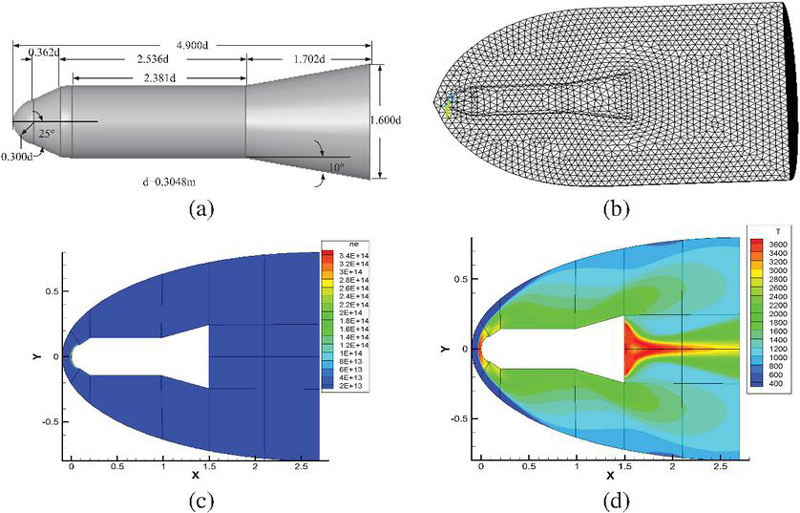
Figure 1 The AGARD HB-2 calibration model at 30 km/10 Ma. (a) Geometric diagram, (b) grid diagram, (c) electron concentration, and (d) temperature.

First, the observation frequency is set to 300 MHz the spatial dispersion size is $\mathrm{\Delta }x=\mathrm{\Delta }y=\mathrm{\Delta }z=0.025$ m, and the time step is set to $\mathrm{\Delta }t=0.7\mathrm{\Delta }x/\sqrt{3}c$, where $c$ represents the propagation speed of electromagnetic waves in free space, the total number of time steps is set to 4000, and the electric field observation point is set at the discrete grid (16, 92, 92). Here, the randomness of electron concentration is considered, assuming that it satisfies the Gaussian probability distribution and the mean value satisfies the spatial distribution shown in Fig. 1. The mean value and standard deviation of electron concentration at different spatial locations are different, their ratio is assumed to be the same, and the standard deviation/mean value equals 2%. Monte Carlo method and CFDTD method based on PCE technology (PCE-CFDTD) were used for uncertainty analysis. The sampling times of Monte Carlo method was 100 times, and the polynomial order of PCE technology was set as $p=1$. Figure 2 shows the expected and standard deviation of the electric field at the observation points of the two methods, which are in good agreement, indicating the correctness of the proposed PCE-CFDTD. Figure 3 shows the comparison diagram of the bistatic RCS mean value of the target at 300 MHz. In order to further prove the effectiveness of PCE technology, the calculation time of the two methods is listed in Table 1. The Monte Carlo method with 100 samples takes 114,698 s, while the proposed PCE-CFDTD method takes only 5,901 s, which greatly saves calculation time. Results show the high efficiency of the proposed PCE-CFDTD method.

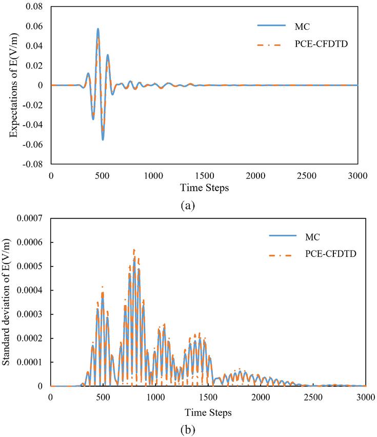
Figure 2 Comparison of electric field results at the observation point of different methods. (a) Expectations and (b) standard deviation.

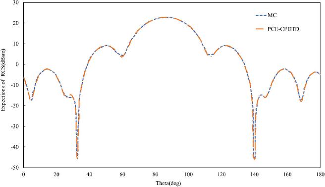
Figure 3 Expectations of RCS at 300 MHz.

Table 1 CPU time comparison

Method	MC	PCE-CFDTD
CPU time(s)	114,698	5,901

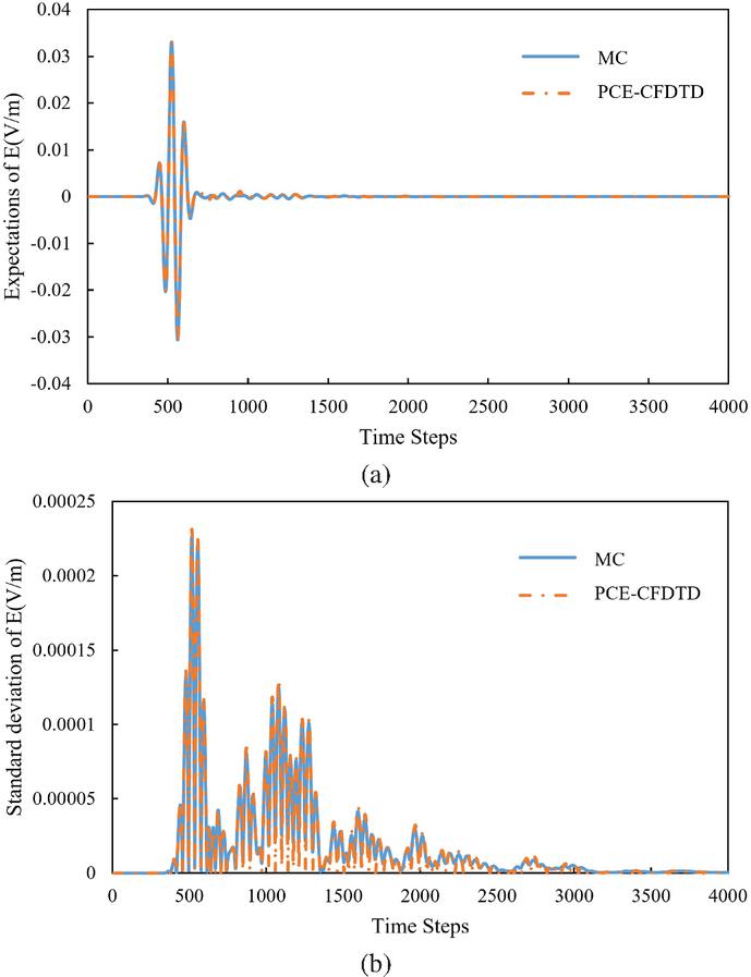
Figure 4 Comparison of electric field results at the observation point of different methods. (a) Expectations and (b) standard deviation.

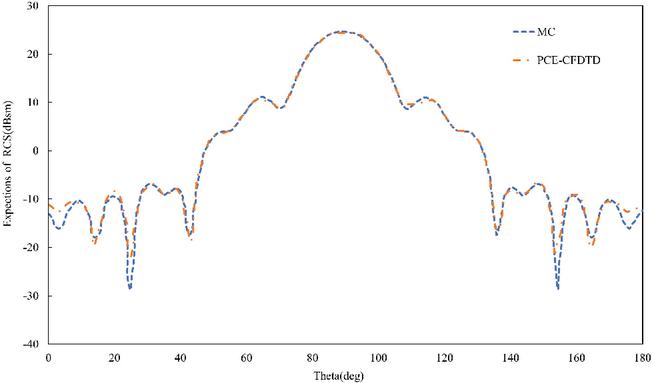
Figure 5 Expectation comparison of RCS at 600 MHz.

Table 2 CPU time comparison

Method	MC	PCE-CFDTD
CPU time(s)	307,315	7583

Next, the observation frequency is set to 600 MHz, the spatial dispersion size is $\mathrm{\Delta }x=\mathrm{\Delta }y=\mathrm{\Delta }z=0.0125$ m, the time step is set to $\mathrm{\Delta }t=0.7\mathrm{\Delta }x/\sqrt{3}c$, and the total number of time steps is set to 3000. The electric field observation point is set at the discrete grid (16, 92, 92), and the randomness of electron concentration is consistent with the above. Figure 4 shows the standard deviation of the electric field at the observation point of the two methods, which is in good agreement. Figure 5 shows a comparison of the mean value of the bistatic RCS of the hypersonic HB-2 model at 600 MHz. Due to the limitation of computer resources and time, the calculation accuracy achieved by Monte Carlo sampling 100 times is not high enough. The calculation time of the two methods is listed in Table 2. The Monte Carlo method with 100 samples takes 307,315 s, while the proposed PCE-CFDTD method only takes 7,583 s, which greatly saves calculation time. Results show the high efficiency of the proposed PCE-CFDTD method.

5 CONCLUSIONS

In this paper, an efficient algorithm for hypersonic target uncertainty electromagnetic analysis is studied, and the conformal FDTD uncertainty electromagnetic analysis technique based on polynomial chaos expansion is proposed. Firstly, the iterative method of polynomial chaos expansion conformal FDTD method is derived and combined with metal/medium conformal technique and polynomial chaos expansion technique, an efficient electromagnetic analysis of the uncertainty problem of the electron concentration of the plasma generated on the hypersonic target surface is achieved. Currently, this method is limited to solving Maxwell’s equations and has not yet been extended to other equations or to handling the coupling between multiphysics equations.in the future, it could be applied to solve heat conduction equations and address random thermal field problems with uncertain parameters.

REFERENCES

[1] Y. Zheng, I. Jun, and W. Tu, “Overview, progress and next steps for our understanding of the near-earth space radiation and plasma environment: Science and applications,” Advances in Space Research, 2024.

[2] J. Cheng, K. Jin, Y. Kou, R. Hu, and X. Zheng, “An electromagnetic method for removing the communication blackout with a space vehicle upon re-entry into the atmosphere,” J. Appl. Phys., vol. 121, p. 093301, 2017.

[3] N. Mehra, R. K. Singh, and S. C. Bera, “Mitigation of communication blackout during re-entry using static magnetic field,” Prog. Electromag. Res. B, vol. 63, pp. 161–172, 2015.

[4] Y. Hu, Z. Fan, D. Ding, and R. Chen, “Hybrid MLFMA/MLACA for analysis of electromagnetic scattering from inhomogeneous high-contrast objects,” Applied Computational Electromagnetics Society (ACES) Journal, vol. 26, no. 10, pp. 765–772, 2011.

[5] Z. Cong, R. Chen, and Z. He, “Numerical modeling of EM scattering from plasma sheath: A review,” Engineering Analysis with Boundary Elements, vol. 135, pp. 73–92, 2022.

[6] J. Bai, L. Zhang, L. Wang, and T. Wang, “Uncertainty analysis in EMC simulation based on improved method of moments,” Applied Computational Electromagnetics Society (ACES) Journal, vol. 31, no. 1, pp. 66–71, 2016.

[7] A. Drandiæ and B. Trkulja, “Computation of electric field inside substations with boundary element methods and adaptive cross approximation,” Engineering Analysis with Boundary Elements, vol. 91, pp. 1–6, 2018.

[8] J. Bai, B. Hu, and A. Duffy, “Uncertainty analysis for EMC simulation based on Bayesian optimization,” IEEE Transactions on Electromagnetic Compatibility, vol. 67, no. 2, pp. 587–597, Apr. 2025.

[9] E. Garcia, “Electromagnetic compatibility uncertainty, risk, and margin management,” IEEE Transactions on Electromagnetic Compatibility, vol. 52, no. 1, pp. 3–10, Feb. 2010.

[10] G. S. Fishman, Monte Carlo. Concepts, Algorithms, and Applications. New York, NY, USA: Springer, 1996.

[11] F. D. Hastings, J. B. Schneider, and S. L. Broschat, “A Monte-Carlo FDTD technique for rough surface scattering,” IEEE Transactions on Antennas and Propagation, vol. 43, no. 11, pp. 1183–1191, Nov. 1995.

[12] K. M. Bisheh, B. Zakeri, and S. M. H. Andargoli, “Correlation coefficient estimation for stochastic FDTD method,” International Symposium on Telecommunications, pp. 234–238, 2014.

[13] S. M. Smith and C. Furse, “Stochastic FDTD for analysis of statistical variation in electromagnetic fields,” IEEE Transactions on Antennas and Propagation, vol. 60, no. 7, pp. 3343–3350, July 2012.

[14] S. M. Smith, “Stochastic finite-difference time-domain,” Ph.D. dissertation, Dept. Elect. Eng, Univ. Utah, Salt Lake City, UT, USA, 2011.

[15] B. T. Nguyen, C. Furse, and J. J. Simpson, “A 3-D stochastic FDTD model of electromagnetic wave propagation in magnetized ionosphere plasma,” IEEE Transactions on Antennas and Propagation, vol. 63, no. 1, pp. 304–313, Jan. 2015.

[16] J. Silly-Carette, D. Lautru, M. F. Wong, A. Gati, J. Wiart, and V. F. Hanna, “Variability on the propagation of a plane wave using stochastic collocation methods in a bio electromagnetic application,” IEEE Microwave and Wireless Components Letters, vol. 19, no. 4, pp. 185–187, Apr. 2009.

[17] R. S. Edwards, A. C. Marvin, and S. J. Porter, “Uncertainty analyses in the finite-difference time-domain method,” IEEE Transactions on Electromagnetic Compatibility, vol. 52, no. 1, pp. 155–163, Feb. 2010.

[18] A. C. M. Austin and C. D. Sarris, “Efficient analysis of geometrical uncertainty in the FDTD method using polynomial chaos with application to microwave circuits,” IEEE Transactions on Microwave Theory and Techniques, vol. 61, no. 12, pp. 4293-4301, 2013.

[19] G. G. Pyrialakos, T. T. Zygiridis, and N. V. Kantartzis, “A 3-D polynomial-chaos FDTD technique for complex inhomogeneous media with arbitrary stochastically-varying index gradients,” Applied Computational Electromagnetics Society (ACES) Journal, vol. 1, no. 3, pp. 109–112, 2016.

[20] X. Lin, W. Zheng, and F. Huang, “Uncertainty quantification and robust shape optimization of acoustic structures based on IGA BEM and polynomial chaos expansion,” Engineering Analysis with Boundary Elements, vol. 165, p. 105770, 2024.

[21] C. Jiang, Y. Qi, and E. Shi, “Combination of Karhunen-Loève and intrusive polynomial chaos for uncertainty quantification of thermomagnetic convection problem with stochastic boundary condition,” Engineering Analysis with Boundary Elements, vol. 159, pp. 452–465, 2024.

[22] H. Yang, G. Wu, and P. Lyu, “Uncertainty analysis for electromagnetic parameter measurement method of absorbing materials based on waveguide device,” Journal of Electronic Measurement and Instrument, vol. 39, no. 2, pp. 169–176, 2025.

[23] H. Jiang, F. Ferranti, and G. Antonini, “Enhanced sparse polynomial chaos expansion for electromagnetic compatibility uncertainty quantification problems,” IEEE Transactions on Electromagnetic Compatibility, vol. 99, pp. 1–10, Aug. 2025.

BIOGRAPHIES

Yupeng Zhu received the B.S. degree from the Department of Electronic Science, National University of Defense Technology, Changsha, China, in 2003, and the Ph.D. degree in 2009. He is currently a Research Fellow with the Academy of Military Sciences. He has published over 20 papers. His current research interests include radar signal processing, electromagnetic scattering and intelligent sensing technologies.

Dina Chen was born in Taizhou, Jiangsu, China. She received the B.S. degree from the Yancheng Institute of Technology, Yancheng, in 2022. She is currently pursuing the Ph.D. degree in the School of Microelectronics, Nanjing University of Science and Technology (NJUST), Nanjing. Her research interests include computational electromagnetics and microwave power component field-circuit coordination.

Huaguang Bao received the B.S. and Ph.D. degrees in communication engineering from the School of Electrical Engineering and Optical Technique, Nanjing University of Science and Technology, Nanjing, China, in 2011 and 2017, respectively. From 2017 to 2019, he was a Postdoctoral Fellow in the Computational Electromagnetics and Antennas Research Laboratory, Department of Electrical Engineering, The Pennsylvania State University, USA. He is currently a Professor with the Department of Integrated Circuit Engineering, Nanjing University of Science and Technology. His research interests include semiconductor simulation, RF-integrated circuits, and computational electromagnetics.

Min Han received the M.S. degree in information and communication engineering from the Nanjing University of Science and Technology, Nanjing, China, in 2013, and the Ph.D. degree in electromagnetic field and microwave engineering from Southeast University, Nanjing, in 2020. She is currently an Associate Researcher at the Academy of Military Sciences. Her research interests include electromagnetic scattering, millimeter wave circuits, and radar signal processing.

ACES JOURNAL, Vol. 40, No. 10, 962–970
DOI: 10.13052/2025.ACES.J.401001
© 2025 River Publishers