A PEC Conformal FDTD Algorithm with Distorted Grid Face Filtering for Enhanced Efficiency

Chenshu Liu, Kaihang Fan, and Juan Chen

School of Information and Communications Engineering
Xi’an Jiaotong University, Xi’an 710049, China
Shelleylcs@stu.xjtu.edu.cn, khfan@xjtu.edu.cn, chen.juan.0201@xjtu.edu.cn

Submitted On: August 20, 2025; Accepted On: March 03, 2026

Abstract

The finite-difference time-domain (FDTD) method suffers from accuracy loss when applied to curved targets due to the staircase approximation. To improve the surface fitting accuracy of curved perfect electric conductor (PEC) objects, the conformal finite-difference time-domain (CFDTD) has been introduced. However, when high-precision conformal cell fitting is performed, the time step in CFDTD is significantly reduced by the presence of distorted small cells, leading to much lower computational efficiency. In this paper, a novel PEC CFDTD algorithm with distorted grid face filtering is proposed, which allows a larger time step. By deriving the stability condition of CFDTD, a Conformal Distortion Index (CDI) is defined and used as a filtering criterion. The conformal cells are retained in regions with low CDI, while areas with high CDI are reverted to the staircase mesh. A sensitivity study on a PEC sphere is used to determine an optimal filtering ratio of 5%, under which the proposed method greatly improves computational efficiency while incurring only a minimal loss in accuracy. Numerical examples are presented to validate the effectiveness of the proposed method.

Index Terms: Conformal finite-difference time-domain (CFDTD), curved targets, grid face filtering, time step reduction.

I. INTRODUCTION

The finite-difference time-domain (FDTD) is widely used in computational electromagnetics due to its explicit time-stepping scheme, inherent parallelism, and time-domain broadband response in a single simulation [1, 2, 3, 4]. However, significant staircase errors are introduced in FDTD when discretizing curved perfect electric conductor (PEC) surfaces with Yee cells, which restricts its accuracy in curved target analysis [5, 6, 7]. Conformal FDTD (CFDTD) addresses this issue by employing conformal meshes to fit the curved surfaces for improving modeling accuracy [8]. Nevertheless, high-precision conformal fitting inevitably produces numerous small and highly distorted cells in PEC objects. Because the time step is limited by the smallest cell, the computational efficiency of CFDTD decreases significantly with increasing mesh distortion [9].

To improve the balance between accuracy and efficiency of the CFDTD methods for PEC structures, several schemes have been proposed. Yu and Mittra approximated the area of conformal cells to those of Yee cells, which eases the stability constraint but reduces accuracy [10]. Other methods, such as global mesh adjustment and enlarged cell technique, seek to control distortion or enlarge small cells. This often involves manual intervention or complex field update equations [11, 12, 13, 14]. Mesh modification strategies, such as adjusting edge lengths or shifting intersection points, are used to regularize cell shapes for relaxing the stability constraint [15, 16]. Alternatively, local or multi-rate time stepping schemes have been introduced. This typically requires additional interpolation, thus increasing complexity and computational cost [17, 18]. In these methods, all conformal cells are still preserved, and the restriction imposed by the smallest cells is handled by making the time-stepping scheme or the mesh structure more complicated.

In addition, recent work has extended CFDTD to higher-order and advanced algorithms to further improve stability and enable larger time steps in complex PEC models [19, 20, 21, 22, 23, 24, 25, 26]. Implicit or weakly conditionally stable schemes, such as conformal alternating direction implicit (C-ADI)-FDTD and conformal locally one-dimensional (C-LOD)-FDTD, can formally relax the limit but require solving linear systems at each time step. In practice, C-ADI-FDTD may still suffer from stability degradation on highly distorted conformal meshes. In contrast, C-LOD-FDTD, though unconditionally stable, exhibits relatively large numerical dispersion and may need finer meshes to match the accuracy of explicit CFDTD.

With these advances, CFDTD has continued to mature in recent years, demonstrating improved accuracy, broader applicability, and greater reliability. It has been successfully applied to waveguide ports [9, 27, 28], periodic and anisotropic structures [29], and advanced boundary conditions [30]. These applications underscore the significance of these algorithms and the need for further improvements in computational efficiency and stability, especially for severely distorted meshes.

In this paper, a novel PEC CFDTD algorithm with distorted grid face filtering is proposed. Instead of updating all the highly distorted conformal cells, the proposed method operates directly on the mesh by filtering out a portion of the most problematic cells. By quantitatively relating a Conformal Distortion Index (CDI) to the global time step stability constraint, a filtering criterion is established to replace a preset proportion of highly distorted conformal cells with staircase cells. Thus, a small sacrifice of geometric accuracy for a limited number of cells leads to a much larger allowable time step and a substantial improvement in computational efficiency. A sensitivity study on a PEC sphere identifies 5% as the optimal filtering ratio. Under this setting, the proposed method achieves significant improvement in computational efficiency while introducing only a minor accuracy loss compared to the conventional CFDTD, as verified by numerical results.

II. STABILITY ANALYSIS OF CFDTD

When applying the CFDTD method to PEC, conformal meshes truncate the boundary Yee cells. Therefore, the electromagnetic field calculation for the mesh in the boundary region needs to be corrected using Faraday’s law as

$${\oint }_{\partial S}\overrightarrow{E}\cdot \mathit{d}\overrightarrow{l}=-\frac{\partial }{\partial t}{\iint }_S\mu \overrightarrow{H}\cdot \mathit{d}\overrightarrow{S},$$

(1)

where $S$ represents the area of the region, $\partial S$ denotes its boundary, l is the length of the grid cell along the boundary of the region, t is the time, and $\mu$ is the magnetic permeability.

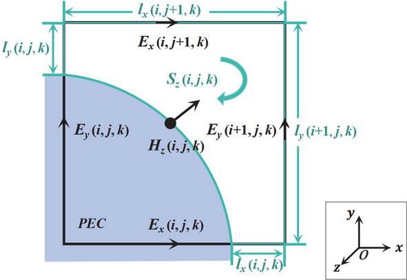
Figure 1 Illustration of changes in conformal mesh integration path and area.

According to equation (1), the explicit magnetic field calculation must be modified to account for changes in the integration path and regions outside the PEC. As shown in Fig. 1, the equation for the z-component of the magnetic field is given as [8]

	$H_z^{n+1/2}(i,j,k)$
	$=H_z^{n-1/2}(i,j,k)+{\displaystyle \frac{\mathrm{\Delta }t}{\mu S_z(i,j,k)}}$
	$\cdot \left[\begin{array}{c}{E}_x^n(i,j+1,k)l_x(i,j+1,k)\hfill \\ -E_x^n(i,j,k)l_x(i,j,k)\hfill \\ -E_y^n(i+1,j,k)l_y(i+1,j,k)\hfill \\ +E_y^n(i,j,k)l_y(i,j,k)\hfill \end{array}\right],$	(2)

where $\mathrm{\Delta }t$ denotes the time step size. At the grid point with three-dimensional coordinates $(i,j,k)$, $S_z(i,j,k)$ represents the area of the $H_z$-associated grid cell outside the PEC, $l_x$, $l_y$ denote the lengths of the grid edges along the x and y directions at the boundary of $S_z(i,j,k)$ outside the PEC, and n is the time step index.

To preserve the finite-difference formulation of the magnetic field components along different coordinate directions in CFDTD, equivalent edge lengths $l_v^{\prime }$ and equivalent areas $S_v^{\prime }(v=x,y,z)$ are introduced. Using the magnetic field component in the z-direction, illustrated in Fig. 1 as an example, we define

$$l_x^{\prime }=l_x/\mathrm{\Delta }x,l_y^{\prime }=l_y/\mathrm{\Delta }y,S_z^{\prime }=S/\mathrm{\Delta }x\mathrm{\Delta }y,$$

(3)

where $\mathrm{\Delta }v(v=x,y,z)$ denotes the full sizes of the Yee cells in the x, y, and z directions, respectively, representing the differential discretization intervals along each axis.

Thus, the equivalent edge lengths of the conformal cell are $l_x^{\prime }(i,j+1,k)$ and $l_y^{\prime }(i+1,j,k)$, and the equivalent area is $S_z(i,j,k)$. Consequently, the magnetic field update equation in CFDTD is modified as

	$H_z^{n+1/2}(i,j,k)$
	$=H_z^{n-1/2}(i,j,k)+{\displaystyle \frac{\mathrm{\Delta }t}{\mu S_z^{\prime }(i,j,k)}}$
	$\cdot \left[\begin{array}{c}{\displaystyle \frac{{\mathrm{E}}_{\mathrm{x}}^{\mathrm{n}}(\mathrm{i},\mathrm{j}+1,\mathrm{k}){\mathrm{l}}_{\mathrm{x}}^{\prime }(\mathrm{i},\mathrm{j}+1,\mathrm{k})-{\mathrm{E}}_{\mathrm{x}}^{\mathrm{n}}(\mathrm{i},\mathrm{j},\mathrm{k}){\mathrm{l}}_{\mathrm{x}}^{\prime }(\mathrm{i},\mathrm{j},\mathrm{k})}{\mathrm{\Delta }\mathrm{y}}}\hfill \\ {\displaystyle \frac{{\mathrm{E}}_{\mathrm{y}}^{\mathrm{n}}(\mathrm{i},\mathrm{j},\mathrm{k}){\mathrm{l}}_{\mathrm{y}}^{\prime }(\mathrm{i},\mathrm{j},\mathrm{k})-{\mathrm{E}}_{\mathrm{y}}^{\mathrm{n}}(\mathrm{i}+1,\mathrm{j},\mathrm{k}){\mathrm{l}}_{\mathrm{y}}^{\prime }(\mathrm{i}+1,\mathrm{j},\mathrm{k})}{\mathrm{\Delta }\mathrm{x}}}\hfill \end{array}\right].$	(4)

While the magnetic field is adjusted in the CFDTD method, the electric field calculation still follows the conventional FDTD formulation.

The stability proof of the CFDTD method in this work is based on a simplified form of equation (2). By incorporating all coefficients of the electric field terms in equation (2) into a new definition $E_{v\ast }^n(i,j,k)=E_v^n(i,j,k)\cdot l_v^{\prime }(i,j,k),(v=x,y,z)$, the equation can be rewritten as

	$H_z^{n+1/2}(i,j,k)$
	$=H_z^{n-1/2}(i,j,k)$
	$+{\displaystyle \frac{\mathrm{\Delta }t}{\mu S_z^{\prime }(i,j,k)}}\left[\begin{array}{c}{\displaystyle \frac{E_{x\ast }^n(i,j+1,k)-E_{x\ast }^n(i,j,k)}{\mathrm{\Delta }y}}\hfill \\ -{\displaystyle \frac{E_{y\ast }^n(i+1,j,k)+E_{y\ast }^n(i,j,k)}{\mathrm{\Delta }x}}\hfill \end{array}\right].$	(5)

Considering a linear, isotropic, lossy medium, the fundamental computation equations of CFDTD can be written in matrix form as

	$\left[\begin{array}{cccccc}1& 0& 0& 0& 0& 0\\ 0& 1& 0& 0& 0& 0\\ 0& 0& 1& 0& 0& 0\\ 0& -{\mathrm{C}}_{\mathrm{q}}\cdot {\displaystyle \frac{\partial }{\partial \mathrm{z}}}{\displaystyle \frac{1}{{\mathrm{S}}_{\mathrm{x}}}}& {\mathrm{C}}_{\mathrm{q}}\cdot {\displaystyle \frac{\partial }{\partial \mathrm{y}}}{\displaystyle \frac{1}{{\mathrm{S}}_{\mathrm{x}}}}& 1& 0& 0\\ {\mathrm{C}}_{\mathrm{q}}\cdot {\displaystyle \frac{\partial }{\partial \mathrm{z}}}{\displaystyle \frac{1}{{\mathrm{S}}_{\mathrm{y}}}}& 0& -{\mathrm{C}}_{\mathrm{q}}\cdot {\displaystyle \frac{\partial }{\partial \mathrm{x}}}{\displaystyle \frac{1}{{\mathrm{S}}_{\mathrm{y}}}}& 0& 1& 0\\ -{\mathrm{C}}_{\mathrm{q}}\cdot {\displaystyle \frac{\partial }{\partial \mathrm{y}}}{\displaystyle \frac{1}{{\mathrm{S}}_{\mathrm{z}}}}& {\mathrm{C}}_{\mathrm{q}}\cdot {\displaystyle \frac{\partial }{\partial \mathrm{x}}}{\displaystyle \frac{1}{{\mathrm{S}}_{\mathrm{z}}}}& 0& 0& 0& 1\end{array}\right]$	(6)
	$\times \left[\begin{array}{c}{E}_{x\ast }^{n+1}\\ E_{y\ast }^{n+1}\\ E_{z\ast }^{n+1}\\ H_x^{n+1}\\ H_y^{n+1}\\ H_z^{n+1}\end{array}\right]$	(7)
	$=\left[\begin{array}{cccccc}1& 0& 0& 0& -{\mathrm{C}}_b\cdot {\displaystyle \frac{\partial }{\partial z}}& {\mathrm{C}}_b\cdot {\displaystyle \frac{\partial }{\partial y}}\\ 0& 1& 0& {\mathrm{C}}_b\cdot {\displaystyle \frac{\partial }{\partial z}}& 0& -{\mathrm{C}}_b\cdot {\displaystyle \frac{\partial }{\partial x}}\\ 0& 0& 1& -{\mathrm{C}}_b\cdot {\displaystyle \frac{\partial }{\partial y}}& {\mathrm{C}}_b\cdot {\displaystyle \frac{\partial }{\partial x}}& 0\\ 0& 0& 0& 1& 0& 0\\ 0& 0& 0& 0& 1& 0\\ 0& 0& 0& 0& 0& 1\end{array}\right]$	(8)
	$\times \left[\begin{array}{c}{E}_{x\ast }^n\\ E_{y\ast }^n\\ E_{z\ast }^n\\ H_x^n\\ H_y^n\\ H_z^n\end{array}\right],$	(9)

where $C_b=\frac{\mathrm{\Delta }t}{\epsilon },C_q=\frac{\mathrm{\Delta }t}{\mu }$, and $\epsilon$ is the dielectric constant.

The field components $E^n$ and $H^n$ in equation (2) can be represented as three-dimensional plane waves at time step n

$$\{\begin{array}{c}{E}^n={\varphi }_E{\zeta }^n\exp [j(k_{x}x+k_{y}y+k_{z}z)]\\ H^n={\varphi }_H{\zeta }^n\exp [j(k_{x}x+k_{y}y+k_{z}z)]\end{array},$$

(10)

where $\varphi$ is the amplitude of the field components, $\zeta$ is the amplification factor, and $k_x,k_y,k_z$ are the wavenumbers in the x, y, z directions, respectively.

Substituting equation (42) into equation (20) and discretizing the spatial components $\exp [j(k_{x}x+k_{y}y+k_{z}z)$ gives

	$\left[\begin{array}{cccccc}\zeta -1& 0& 0& 0& {\mathrm{C}}_{\mathrm{bx}}^{\prime }{\sigma }_{\mathrm{z}}& -{\mathrm{C}}_{\mathrm{bx}}^{\prime }{\sigma }_{\mathrm{y}}\\ 0& \zeta -1& 0& -{\mathrm{C}}_{\mathrm{by}}^{\prime }{\sigma }_{\mathrm{z}}& 0& {\mathrm{C}}_{\mathrm{by}}^{\prime }{\sigma }_{\mathrm{x}}\\ 0& 0& \zeta -1& {\mathrm{C}}_{\mathrm{bz}}^{\prime }{\sigma }_{\mathrm{y}}& -{\mathrm{C}}_{\mathrm{bz}}^{\prime }{\sigma }_{\mathrm{x}}& 0\\ 0& -\zeta {\mathrm{C}}_{\mathrm{qx}}^{\prime }\cdot {\sigma }_{\mathrm{z}}& \zeta {\mathrm{C}}_{\mathrm{qx}}^{\prime }{\sigma }_{\mathrm{y}}& \zeta -1& 0& 0\\ \zeta {\mathrm{C}}_{\mathrm{qy}}^{\prime }{\sigma }_{\mathrm{z}}& 0& -\zeta {\mathrm{C}}_{\mathrm{qy}}^{\prime }{\sigma }_{\mathrm{x}}& 0& \zeta -1& 0\\ -\zeta {\mathrm{C}}_{\mathrm{qz}}^{\prime }{\sigma }_{\mathrm{y}}& \zeta {\mathrm{C}}_{\mathrm{qz}}^{\prime }{\sigma }_{\mathrm{x}}& 0& 0& 0& \zeta -1\end{array}\right]$	(11)
	$\cdot \left[\begin{array}{c}{\varphi }_{E_x}{\zeta }_n\\ {\varphi }_{E_y}{\zeta }_n\\ {\varphi }_{E_z}{\zeta }_n\\ {\varphi }_{H_x}{\zeta }_n\\ {\varphi }_{H_y}{\zeta }_n\\ {\varphi }_{H_z}{\zeta }_n\end{array}\right]=0,$	(12)

where ${\sigma }_x=2j\sin \left(\frac{k_x\mathrm{\Delta }x}{2}\right)/\mathrm{\Delta }x$, ${\sigma }_y=2j\sin \left(\frac{k_y\mathrm{\Delta }y}{2}\right)/\mathrm{\Delta }y$, ${\sigma }_z=2j\sin \left(\frac{k_z\mathrm{\Delta }z}{2}\right)/\mathrm{\Delta }z$, $C_{bv}^{\prime }=\frac{\mathrm{\Delta }t\cdot l_v^{\prime }}{\epsilon }$, $C_{qv}^{\prime }=\frac{\mathrm{\Delta }t}{\mu \cdot S_v^{\prime }}$, $(v=x,y,z)$.

For equation (49) to have non-trivial solutions, the determinant of the coefficient matrix must be zero, that is

$${(\zeta -1)}^2{\left[\begin{array}{c}\zeta (C_{bx}^{\prime }{C}_{qx}^{\prime }{\sigma }_x^2+C_{by}^{\prime }{C}_{qy}^{\prime }{\sigma }_y^2+C_{bz}^{\prime }{C}_{qz}^{\prime }{\sigma }_z^2)\hfill \\ -(\zeta -1)(\zeta -1)\hfill \end{array}\right]}^2=0.$$

(13)

To ensure numerical stability during iterative computation, the amplitude of the amplification factor must satisfy $|\zeta |=1$, thus, equation (57) is equivalent to

$$\zeta -1=0,$$	(14)
$$\zeta (C_{bx}^{\prime }{C}_{qx}^{\prime }{\sigma }_x^2+C_{by}^{\prime }{C}_{qy}^{\prime }{\sigma }_y^2+C_{bz}^{\prime }{C}_{qz}^{\prime }{\sigma }_z^2)-{(\zeta -1)}^2=0.$$	(15)

By solving equation (58), we obtain $|\zeta |=|1|\le 1$, indicating that this stability condition is always satisfied. Equation (59) can then be rearranged as

$${\zeta }^2-[2+C_{bx}^{\prime }{C}_{qx}^{\prime }{\sigma }_x^2+C_{by}^{\prime }{C}_{qy}^{\prime }{\sigma }_y^2+C_{bz}^{\prime }{C}_{qz}^{\prime }{\sigma }_z^2]\zeta +1=0.$$

(16)

For the convenience of calculation, a linear transformation defined by $\zeta =\frac{r+1}{r-1}$ is applied to equation (60) as

	$[-C_{bx}^{\prime }{C}_{qx}^{\prime }{\sigma }_x^2+C_{by}^{\prime }{C}_{qy}^{\prime }{\sigma }_y^2+C_{bz}^{\prime }{C}_{qz}^{\prime }{\sigma }_z^2]r^2$
	$+[4+C_b^{\prime }{C}_q^{\prime }({\sigma }_x^2+{\sigma }_y^2+{\sigma }_z^2)]=0.$	(17)

Using the Routh-Hurwitz criterion [31], the necessary and sufficient condition for numerical stability in equation (2) is that all coefficients are positive. The first-order terms are always positive, so only the constant term requires further analysis, which is simplified as

	$\left[\begin{array}{c}{\displaystyle \frac{l_x^{\prime }}{S_x^{\prime }}}\cdot {\left({\displaystyle \frac{\sin \left(\frac{k_x\mathrm{\Delta }x}{2}\right)}{\mathrm{\Delta }x}}\right)}^2+{\displaystyle \frac{l_y^{\prime }}{S_y^{\prime }}}\cdot {\left({\displaystyle \frac{\sin \left(\frac{k_y\mathrm{\Delta }y}{2}\right)}{\mathrm{\Delta }y}}\right)}^2\hfill \\ +{\displaystyle \frac{l_z^{\prime }}{S_z^{\prime }}}\cdot {\left({\displaystyle \frac{\sin \left(\frac{k_z\mathrm{\Delta }z}{2}\right)}{\mathrm{\Delta }z}}\right)}^2\hfill \end{array}\right]$	(18)
	$\le \left[{\displaystyle \frac{l_x^{\prime }}{S_x^{\prime }}}{\left({\displaystyle \frac{1}{\mathrm{\Delta }x}}\right)}^2+{\displaystyle \frac{l_y^{\prime }}{S_y^{\prime }}}{\left({\displaystyle \frac{1}{\mathrm{\Delta }y}}\right)}^2+{\displaystyle \frac{l_z^{\prime }}{S_z^{\prime }}}{\left({\displaystyle \frac{1}{\mathrm{\Delta }z}}\right)}^2\right]\le {\displaystyle \frac{\epsilon \mu }{{\left(\mathrm{\Delta }t\right)}^2}}.$	(19)

Accordingly, the time step $\mathrm{\Delta }t$ in CFDTD should meet the following criterion

$\mathrm{\Delta }{t}_{CFDTD}$	$\le \sqrt{{\displaystyle \frac{\epsilon \mu }{\frac{l_x^{\prime }}{S_x^{\prime }}{\left(\frac{1}{\mathrm{\Delta }x}\right)}^2+\frac{l_y^{\prime }}{S_y^{\prime }}{\left(\frac{1}{\mathrm{\Delta }y}\right)}^2+\frac{l_z^{\prime }}{S_z^{\prime }}{\left(\frac{1}{\mathrm{\Delta }z}\right)}^2}}}$
	$\le \sqrt{{\displaystyle \frac{\epsilon \mu }{{\left(\frac{l^{\prime }}{S^{\prime }}\right)}_{\max (x,y,z)}\left[{\left(\frac{1}{\mathrm{\Delta }x}\right)}^2+{\left(\frac{1}{\mathrm{\Delta }y}\right)}^2+{\left(\frac{1}{\mathrm{\Delta }z}\right)}^2\right]}}}$
	$=\mathrm{\Delta }{t}_{FDTD}/{\left(\sqrt{{\displaystyle \frac{l^{\prime }}{S^{\prime }}}}\right)}_{\max (x,y,z)}.$	(20)

In summary, the stability condition for the CFDTD method is $\mathrm{\Delta }{t}_{CFDTD}\le \mathrm{\Delta }{t}_{FDTD}/{(\sqrt{\frac{l^{\prime }}{S^{\prime }}})}_{\max }$.

III. IMPLEMENTATION OF CFDTD BASED ON DISTORTED MESH SURFACES FILTERING

A. Conformal Distortion Index

As discussed in Section II, the conformal treatment of PEC boundaries modifies the effective edge lengths and areas of the truncated Yee cells, and these equivalent geometric parameters enter the stability condition in (2). In this paper, we introduce the CDI to characterize the distortion of conformal mesh surfaces in a way that is directly linked to this stability constraint.

The CDI of a conformal mesh surface is calculated as shown in Fig. 2. Here, $l_a^{\prime }$, $l_b^{\prime }$, $l_c^{\prime }$, and $l_d^{\prime }$ are the equivalent lengths of the mesh surface’s four edges, respectively, and S represents the equivalent area.

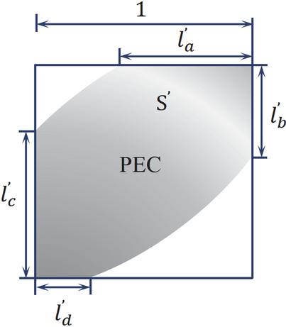
Figure 2 Illustration of CDI parameter analysis for the conformal mesh surface.

Hence, the defined CDI in a conformal mesh surface can be expressed as

$CDI={(\sqrt{l^{\prime }/S^{\prime }})}_{\max }=\sqrt{\max (l_a^{\prime },l_b^{\prime },l_c^{\prime },l_d^{\prime })/S^{\prime }}=\sqrt{l_c^{\prime }/S^{\prime }}.$

(21)

Substituting (67) into (2), the numerical stability condition for CFDTD can be expressed as

$$\mathrm{\Delta }{t}_{CFDTD}\le \mathrm{\Delta }{t}_{FDTD}/CD{I}_{\max },$$

(22)

where $CD{I}_{max}$ refers to the maximum CDI among all conformal mesh surfaces. For a given conformal cell surface, the time step is limited by $CD{I}_{max}$. According to [11], it can be seen that $CD{I}_{max}\ge 1$. As the $CD{I}_{max}$ of the conformal cell increases, the time step will be smaller and, consequently, the computational efficiency in CFDTD is also reduced.

Unlike conventional mesh-quality metrics, CDI is constructed directly from the equivalent edge lengths and equivalent area so that it appears explicitly in the CFDTD stability constraint in (68), and therefore quantitatively describes how strongly the most distorted conformal surfaces restrict the global time step. To alleviate this limitation, a novel CFDTD method with distorted grid surface filtering is proposed to remove highly distorted conformal cell surfaces, thereby reducing the overall $CD{I}_{max}$.

B. Specific implementation

The proposed PEC CFDTD with distorted grid surface filtering proceeds as follows.

(a) Calculate the CDI for all conformal cell surfaces using (67) and rank them in descending order to create a priority list for filtering.

(b) Set the removal ratio $\eta$ and remove the top $\eta$ fraction of the distorted surfaces from the list. Removed mesh cells are converted back to regular grid cells based on the dielectric properties at their centers, aiming to preserve the geometric integrity as much as possible.

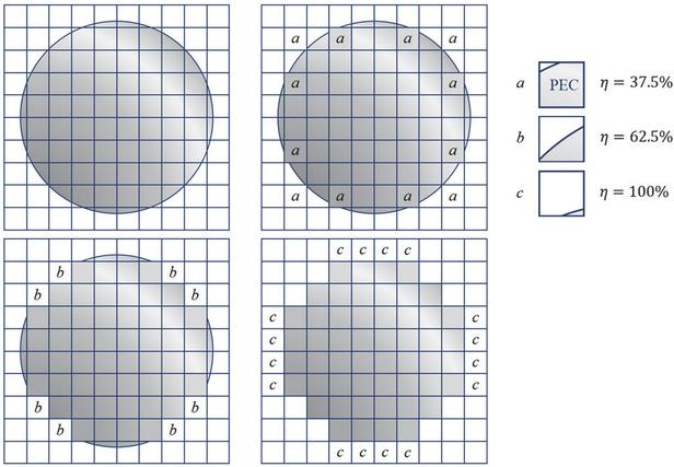
Figure 3 Illustration of the proposed CFDTD method incorporating distorted grid surface filtering.

To clarify the proposed approach, a two-dimensional circular PEC surface, shown in Fig. 3, was constructed and discretized using conformal meshing. For this model, the filtering procedure was applied to conformal meshes, which are divided into filtering regions a, b, and c according to descending CDI values. At a removal ratio $\eta$ of 37.5%, cells in region a are reverted to the conventional Yee cell; increasing $\eta$ to 62.5% includes region b as well, thereby filtering out meshes with moderate CDI values. When $\eta$ reaches 100%, region c is also converted back to the base mesh, so that subsequent calculations are performed entirely on the standard FDTD grid.

After applying a certain proportion of filtering to the mesh using this method, the maximum time step for the proposed method is then given by

$\mathrm{\Delta }{t}_{filtered}$	$=\mathrm{\Delta }{t}_{FDTD}/CD{I}_{\max }^{\prime }$
	$=\mathrm{\Delta }{t}_{FDTD}/{(CD{I}_{\max })}_{\mathit{the}\mathit{remaining}\mathit{grids}}.$	(23)

A larger time step is allowed by increasing the removal ratio, but this may reduce the accuracy of the proposed method. In specific engineering problems, an appropriate ratio can improve computational efficiency significantly within an acceptable range of accuracy loss.

In practical simulations, it is necessary to determine an optimal filtering ratio at which the time step is maximally relaxed while the loss of computational accuracy remains negligible. To identify the optimal filtering ratio, we will perform a detailed parameter sensitivity analysis on typical examples in section IV, thereby establishing a selection criterion for $\eta$ and verifying the effectiveness of the chosen filtering ratio.

IV. NUMERICAL EXAMPLES AND RESULT ANALYSIS

To verify the effectiveness of the proposed PEC CFDTD algorithm based on distorted mesh surface filtering, the radar cross-section (RCS) of two typical curved metal surfaces is analyzed. All simulations are performed on a Windows 10 operating system equipped with an Intel(R) Xeon(R) 8360Y CPU @ 2.40 GHz (up to 3.50 GHz) and 1.0 TB RAM.

A. PEC sphere

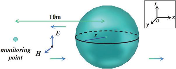
Figure 4 Model for PEC sphere backscattering RCS calculation.

In the first example, a PEC sphere with a radius of 0.36 m is analyzed. An x-polarized plane wave is incident along the positive z-direction, with a Gaussian pulse $f(t)=\exp [-4\pi {(t-t_0)}^2/{\tau }^2]$, where $\tau =2\times {10}^{-9}$ s, $t_0=0.8\tau$. A monitoring point is set at 10 m along the negative z-axis to record the backscattering RCS characteristics of the metal sphere, as shown in Fig. 4.

For an accurate reference solution, the FDTD method uses a uniform small grid of 0.01 m to discretize the metal sphere, while both conventional and proposed CFDTD allow a coarser grid of 0.03 m. The air region adopts a uniform grid of 0.03 m.

The variation of $CD{I}_{max}$ and the average RCS error with respect to the removal ratio $\eta$ is investigated in Fig. 5. When $\eta$ increases from 0% to 5%, $CD{I}_{max}$ drops sharply. Since the time step is inversely proportional to $CD{I}_{max}$, this corresponds to a substantial relaxation of the time step constraint and thus several improvements in computational efficiency. Meanwhile, the RCS curve remains almost unchanged, and the increase in the average error does not exceed 0.1 dB$\cdot$m². When $\eta$ exceeds 5%, the decrease of $CD{I}_{max}$ gradually saturates, so further increasing $\eta$ brings marginal gains in the allowable time step, while the RCS error grows more noticeably. Therefore, $\eta =5\%$ is identified as an effective compromise. The algorithm removes the highly distorted cells that dominate the time step constraint, while keeping the loss of accuracy at a low level.

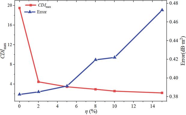
Figure 5 Variations of $CD{I}_{max}$ and average RCS error with respect to removal ratio $\eta$ for the PEC sphere.

To visually verify that this choice is appropriate, Fig. 6 compares the RCS curves for different $\eta$ values. The curve for $\eta =5\%$ almost coincides with CFDTD and the Mie analytical solution, indicating that the proposed method preserves the high accuracy of CFDTD while improving efficiency. In contrast, the RCS curve for $\eta =15\%$ shows clear deviations, implying that excessive filtering destroys the geometric features of the curved surface and deteriorates the scattering response.

Figure 7 further presents the time-domain results of the observation point located 0.03 m from the center of the incident plane wave. The results indicate that for $\eta =15\%$, the time-domain response exhibits noticeable deviations. In contrast, for $\eta =5\%$, it is in good agreement with that of CFDTD throughout the entire simulation time. This confirms both the numerical stability and the accuracy of the proposed method in the time domain.

The detailed simulation parameters and relative errors of the four methods are summarized in Table 1, with the analytical Mie series solution employed as the exact reference. For the conventional CFDTD, the presence of small distorted cells imposes a strict constraint on the time step, leading to an overall runtime even longer than that of the fine mesh FDTD. In contrast, when the proposed filtering strategy with $\eta =5\%$ is applied, the computation time is reduced from 943 s to 151 s, a decrease of about 84.0%. At the same time, the relative error of the backscattering RCS remains around 2.40%, which is essentially comparable to that of the conventional CFDTD. When $\eta$ reaches 15%, the error grows significantly, whereas the gain in computation time becomes negligible.

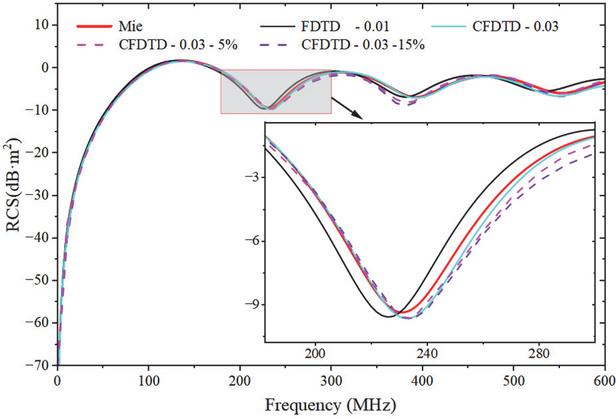
Figure 6 Frequency response of RCS of the PEC sphere.

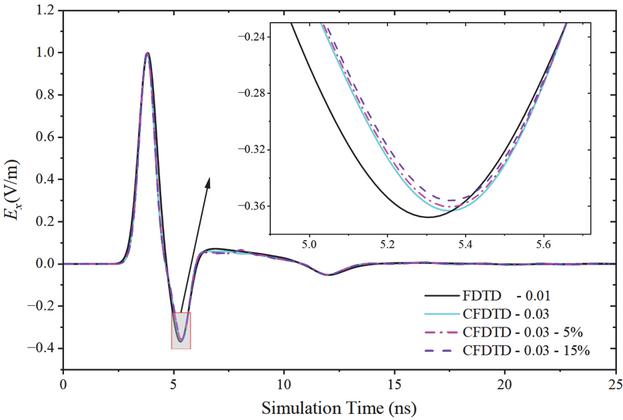
Figure 7 Time-domain results of the PEC sphere.

In summary, for the PEC sphere example, a removal ratio of $\eta =5\%$ provides an almost optimal balance between computational efficiency and accuracy.

Table 1 Comparison of computation parameters for FDTD and proposed methods of the sphere

$\mathit{\eta }$ (%)	Time	Grid	Relative	Memory
	(s)	Number	Error (%)	(MB)
FDTD	1050	438,976	3.99	1400
0	1179	21,952	2.39	549
5	189	21,952	2.40	365
15	133	21,952	2.58	364

B. F117 aircraft model

To further verify the generality of the optimal removal ratio $\eta =5\%$ in complex targets, the F117 aircraft is analyzed. In this example, the aircraft has an overall length of 20.08 m, a height of 3.78 m, and a wingspan of 13.20 m. An x-polarized plane wave at 500 MHz is incident along the positive z-axis, as shown in Fig. 8. The background FDTD domain uses a uniform fine mesh of 0.03 m, while both the conventional CFDTD and the proposed method adopt a grid size of 0.06 m in the conformal region.

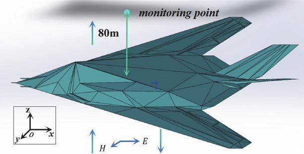
Figure 8 F117 forward RCS computation model.

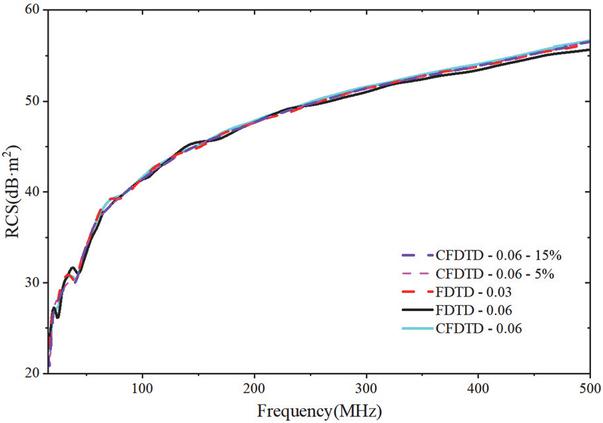
Figure 9 Frequency response of forward RCS for F117.

Figure 9 compares the forward RCS frequency responses obtained by different methods. The results of the proposed filtering method agree very well with those of the conventional CFDTD, while achieving a clear improvement in computational efficiency compared with the fine-mesh FDTD.

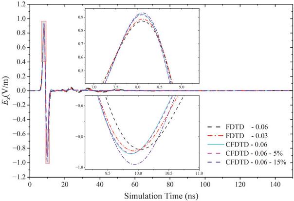
Figure 10 Time-domain results of F117.

The detailed simulation parameters and errors for the five methods applied to the F117 are summarized in Table 2, where the result of the conventional CFDTD is used as the reference. When the recommended removal ratio of 5% is used, the computation time is reduced from 3234 minutes to 651 minutes, corresponding to a 79.9% reduction, while the RCS relative error with respect to the conventional CFDTD is only 1.778%. When the removal ratio is increased to 15%, the computation time is further reduced. However, the additional gain is much less significant than that obtained when increasing the removal ratio from 0% to 5%, while the error continues to increase. This trend is particularly evident in the time-domain results shown in Fig. 10. For a 15% removal ratio, the time-domain result deviates noticeably from CFDTD, while the 5% case still matches it well.

Therefore, choosing a 5% removal ratio for distorted grid faces filtering provides a robust trade-off between accuracy and efficiency, which strongly demonstrates the applicability of the proposed method to electromagnetic simulations of complex targets.

Table 2 Comparison of computation parameters for FDTD and proposed methods of F117

$\mathit{\eta }$ (%)	Time	Grid	Relative	Memory
	(min)	Number	Error (%)	(GB)
FDTD-0.03	1417	22,368,060	1.886	26.25
FDTD-0.06	135	3,025,848	2.582	6.90
0	3234	3,025,848	-	6.95
5	651	3,025,848	1.778	6.93
15	302	3,025,848	2.211	6.91

As shown in the two examples, the proposed CFDTD improves efficiency by filtering part of the distorted grids while keeping the accuracy loss small. As the removal ratio $\eta$ increases, the decrease of the maximum CDI becomes slower. In practice, a removal ratio of about 5% already gives a large gain in the allowable time step and computational efficiency, with only minor error. Therefore, users can choose $\eta$ according to their accuracy and runtime requirements, with $\eta =5\%$ as a recommended optimal choice.

V. CONCLUSION

To improve the computational efficiency of traditional conformal FDTD, this paper proposes a conformal PEC FDTD method with distorted grid-face filtering. A CDI is defined to measure the grid distortion, and a simple statistical filtering scheme is used. Only a small number of conformal cells that impose the most restrictive global time step limit are filtered, which directly relaxes the constraint. Numerical examples for a PEC sphere and an F117 aircraft show that, when the filtering ratio is set to 5%, the proposed method is generally applicable and greatly improves computational efficiency with only a small loss of accuracy. This method provides a simple, robust, and efficient approach for electromagnetic simulation of large and complex targets, allowing users to flexibly balance computational efficiency and geometric modeling accuracy according to practical engineering needs.

ACKNOWLEDGMENT

This work was supported by the National Natural Science Foundation of China Youth Science Fund Project (Category A) under No. 62525114, the National Natural Science Foundation of China Youth Science Fund Project (Category C) under No. 62401455, the Shaanxi Province Innovation Capability Support Plan under No. 2024RS-CXTD-07, and the Key R&D Program of Shaanxi Province under No. 2024GX-ZDCYL-05-04.

REFERENCES

[1] K. S. Yee, “Numerical solution of initial boundary value problems involving Maxwell’s equations,” IEEE Trans. Antennas Propag., vol. 14, no. 3, pp. 302–207, May 1966.

[2] K. S. Kunz and R. J. Luebbers, The Finite-Difference Time-Domain Method for Electromagnetics. Boca Raton, FL, USA: CRC Press, 1993.

[3] A. Taflove and S. C. Hagness, Computational Electrodynamics: The Finite-Difference Time-Domain Method. Norwood, MA, USA: Artech House, 2005.

[4] A. V. Boriskin, A. Rolland, R. Sauleau, and A. I. Nosich, “Assessment of FDTD accuracy in the compact hemielliptic dielectric lens antenna analysis,” IEEE Trans. Antennas Propag., vol. 56, no. 3, pp. 758–764, Mar. 2008.

[5] T. G. Jurgens, A. Taflove, K. Umashankar, and T. G. Moore, “Finite-difference time-domain modeling of curved surfaces,” IEEE Trans. Antennas Propag., vol. 40, no. 4, pp. 357–366, Apr. 1992.

[6] Y. Hao and C. J. Railton, “Analyzing electromagnetic structures with curved boundaries on Cartesian FDTD meshes,” IEEE Trans. Microw. Theory Techn., vol. 46, no. 1, pp. 82–88, Jan. 1998.

[7] A. C. Cangellaris and D. B. Wright, “Analysis of the numerical error caused by the stair-stepped approximation of a conducting boundary in FDTD simulations of electromagnetic phenomena,” IEEE Trans. Antennas Propag., vol. 39, no. 10, pp. 1518–1525, Oct. 1991.

[8] S. Dey and R. Mittra, “A locally conformal finite-difference time-domain (CFDTD) algorithm for modeling three-dimensional perfectly conducting objects,” IEEE Microw. Guided Wave Lett., vol. 17, no. 9, pp. 273–275, Sep. 1997.

[9] G. Chen, J. Stang, and M. Moghaddam, “A conformal FDTD method with accurate waveport excitation and S-parameter extraction,” IEEE Trans. Antennas Propag., vol. 64, no. 10, pp. 4504–4509, Oct. 2016.

[10] W. Yu and R. Mittra, “A conformal FDTD algorithm for modeling perfectly conducting objects with curve-shaped surfaces and edges,” Microw. Opt. Technol. Lett., vol. 27, no. 2, pp. 136–138, Aug. 2000.

[11] S. Benkler, N. Chavannes, and N. Kuster, “A new 3-D conformal PEC FDTD scheme with user-defined geometric precision and derived stability criterion,” IEEE Trans. Antennas Propag., vol. 54, no. 6, pp. 1843–1849, June 2006.

[12] T. Xiao and Q. H. Liu, “Enlarged cells for the conformal FDTD method to avoid the time step reduction,” IEEE Microw. Wireless Compon. Lett., vol. 14, no. 12, pp. 551–553, Dec. 2004.

[13] R. Schuhmann, I. A. Zagorodnov, and T. Weiland, “Comment on ‘Enlarged cells for the conformal FDTD method to avoid the time step reduction,”’ IEEE Microw. Wireless Compon. Lett., vol. 16, no. 1, p. 55, Jan. 2006.

[14] T. Xiao and Q. H. Liu, “A 3-D enlarged cell technique (ECT) for the conformal FDTD method,” IEEE Trans. Antennas Propag., vol. 56, no. 3, pp. 765–773, Mar. 2008.

[15] I. A. Zagorodnov, R. Schuhmann, and T. Weiland, “Conformal FDTD method to avoid time step reduction with and without cell enlargement,” J. Computational Phys., vol. 225, pp. 1493–1507, Aug. 2007.

[16] M. R. Cabello, L. D. Angulo, J. Alvarez, A. R. Bretones, G. G. Gutierrez, and S. G. Garcia, “A new efficient and stable 3D conformal FDTD,” IEEE Microw. Wireless Compon. Lett., vol. 26, no. 8, pp. 553–555, Aug. 2016.

[17] C. M. Kuo and C. W. Kuo, “A new scheme for the conformal FDTD method to calculate the radar cross-section of perfect conducting curved objects,” IEEE Antennas Wireless Propag. Lett., vol. 9, pp. 16–19, 2010.

[18] C.-M. Kuo and C.-W. Kuo, “A novel FDTD time-stepping scheme to calculate RCS of curved conducting objects using adaptively adjusted time steps,” IEEE Trans. Antennas Propag., vol. 61, no. 10, pp. 5127–5134, Oct. 2013.

[19] M. Chai, T. Xiao, and Q. H. Liu, “Conformal method to eliminate the ADI-FDTD staircasing errors,” IEEE Trans. Electromagn. Compat., vol. 48, no. 2, pp. 273–281, May 2006.

[20] J. Dai, Z. Chen, D. Su, and X. Zhao, “Stability analysis and improvement of the conformal ADI-FDTD methods,” IEEE Trans. Antennas Propag., vol. 59, no. 6, pp. 2248–2258, June 2011.

[21] J. Wang and W. Y. Yin, “Development of a novel FDTD (2, 4)-compatible conformal scheme for electromagnetic computations of complex curved PEC objects,” IEEE Trans. Antennas Propag., vol. 61, no. 1, pp. 299–309, Jan. 2013.

[22] W. Shi, J. Wang, Q.-F. Liu, W.-J. Wu, and W.-Y. Yin, “A conformal scheme for modeling curved dispersive medium objects compatible with ADE-FDTD (2, 4) method,” IEEE Antennas Wireless Propag. Lett., vol. 24, no. 1, pp. 177–181, Jan. 2025.

[23] X. Wei, W. Shao, S. Shi, Y. Zhang, and B. Wang, “An efficient locally one-dimensional finite-difference time-domain method based on the conformal scheme,” Chin. Phys. B, vol. 24, no. 7, pp. 76–84, May 2015.

[24] H. Liu, X. Zhao, X.-H. Wang, S. Yang, and Z. Chen, “An unconditionally stable conformal LOD-FDTD method for curved PEC objects and its application to EMC problems,” IEEE Trans. Electromagn. Compat., vol. 64, no. 3, pp. 827–839, June 2022.

[25] M. Zhu, Q. Cao, L. Zhao, and X. Li, “Analysis of three-dimensional curved objects by Runge-Kutta high-order time-domain method,” Appl. Comput. Electromagn., vol. 30, no. 1, pp. 86–92, 2015.

[26] M. A. Kourah, M. F. Hadi, and A. S. Al-Zayed, “Extending the enlarged cell and uniformly stable conformal techniques to modeling curved conductors in two-dimensional high-order finite-difference time-domain algorithms,” Int. J. Numer. Model. Electron. Netw. Devices Fields, vol. 26, no. 3, pp. 205–306, May 2013.

[27] K. Wang, S. Zuo, Q. Wu, Z. Lin, Y. Zhang, and X. Zhao, “A novel compact conformal 2-D FDFD method for modeling waveports in 3-D FDTD,” IEEE Antennas Wireless Propag. Lett., vol. 23, no. 7, pp. 2091–2095, July 2024.

[28] G. Lin, T. Huang, W. Cai, D. Gong, and X. Jin, “An efficient scheme of waveguide port modeling based on conformal and nonuniform mesh for time-domain finite integration technique,” IEEE Trans. Antennas Propag., vol. 73, no. 2, pp. 1047–1058, Feb. 2025.

[29] K. Wang, Q. Wu, F. Yu, S. Zuo, Z. Lin, X. Zhao, and Y. Zhang, “Conformal anisotropic periodic boundary condition for FDTD method,” IEEE Antennas Wireless Propag. Lett., vol. 24, no. 1, Jan. 2025.

[30] S. Gaucher, C. Guiffaut, N. Bui, A. Reineix, and O. Cessenat, “Angle-dependent face-centered SIBC model of metamaterial in conformal FDTD methods,” IEEE Trans. Antennas Propag., vol. 71, no. 9, pp. 7438–7446, Sep. 2023.

[31] A. Pereda, L. A. Vielva, A. Vegas, and A. Prieto, “Analyzing the stability of the FDTD technique by combining the von Neumann method with the Routh-Hurwitz criterion,” IEEE Trans. Microw. Theory Tech., vol. 49, no. 2, pp. 377–381, Feb. 2001.

BIOGRAPHIES

Chenshu Liu was born in Hubei, China, in 2002. She received her B.S. degree in Electronic and Information Engineering from Xi’an Jiaotong University, Xi’an, in 2024, where she is currently working toward an M.S. degree in Electromagnetic Field and Microwave Technology. Her current research interests include computational electromagnetics.

Kaihang Fan received the B.S. degree in electronic information science and technology from Xidian University, Xi’an, China, in 2014, and the Ph.D. degree in radio physics, Xidian University, Xi’an, in 2021. She is currently an Assistant Professor with the School of Information and Communications Engineering, Xi’an Jiaotong University, Xi’an. Her current research interests include computational electromagnetics numerical methods and multi-physics field simulation.

Juan Chen was born in Chongqing, China. She received the Ph.D. degree from Xi’an Jiaotong University, Xi’an, in 2008, in electromagnetic field and microwave technology. She is currently working in Xi’an Jiaotong University, Xi’an, as a professor. Her research interests include computational electromagnetics and microwave device design.

ACES JOURNAL, Vol. 41, No. 3, 216–224
DOI: 10.13052/2026.ACES.J.410303
© 2026 River Publishers