Numerical Analysis of Large-Scale Phased Array Calibration, Using a Kronecker Product Formulation

Jake W. Liu

Department of Electronic Engineering, National Taipei University of Technology, Taipei 10608, Taiwan, jwliu@ntut.edu.tw

Submitted On: August 15, 2025; Accepted On: February 10, 2026

Abstract

This paper proposes a calibration method for large-scale phased arrays based on a Kronecker product formulation, termed the Kronecker Product Method (KPM). Unlike the conventional Phase Toggling Method (PTM), which excites one element per measurement and suffers from limited measurement diversity, KPM employs simultaneous binary-phase excitation across all elements. This structure enhances robustness against noise and error accumulation, particularly in large arrays or high Signal-to-Noise Ratio (SNR) conditions. KPM retains PTM’s simplicity and 1-bit phase control compatibility while offering superior theoretical properties and practical performance.

Keywords: Far-field calibration method, Kronecker product, large arrays, phase toggling method, phased array calibration..

1 INTRODUCTION

Accurate calibration is essential for phased arrays, especially in applications demanding precise beamforming and null control [1, 2, 3, 4]. Practical systems suffer from phase and amplitude errors, requiring calibration to maintain pattern fidelity.

Early techniques used near-field scans [5, 6], later improved by PWS-based Backward Transformation Methods (BTM) [7, 8, 9], but both are complex and scale poorly. In contrast, far-field methods offer better efficiency in calibration since no mechanical scan is required. Among these, the Phase Toggling Method (PTM) [10] is widely used due to its simplicity and compatibility with 1-bit digital phase shifters (DPSs). However, its element-wise toggling leads to poor signal diversity and degraded performance in large arrays or high-SNR conditions. Rotating-Element Electric-Field Vector Method (REVM) [11] offers phase-free calibration using total field magnitudes, enabling amplitude-only measurements.

Recent works improve efficiency via structured, multi-element excitations [12, 13, 14]. Multiple REVM [14] uses Fourier decomposition but is limited by model and resolution. Group-wise amplitude-only methods [15] enhance low-SNR performance. Others employ binary-phase modulation and harmonic analysis [16] or optimize matrix design [17]. A general framework in [18] builds excitation matrices recursively. While the proposed method shares this formulation, it differs by systematically constructing the excitation matrix as a Kronecker product of a 2×2 Hadamard base, offering compactness, scalability, and tractable error analysis.

Despite recent advances, PTM remains a baseline for its simplicity and binary control. Its limited diversity, however, constrains scalability. The proposed Kronecker Product Method (KPM) addresses this by enabling joint multi-element modulation using a structured matrix that remains linearly independent across array sizes. Like PTM, KPM uses only 0 and $\pi$ phase shifts, preserving hardware simplicity and making it suitable for low-bit systems [19, 20, 21].

The rest of the paper is organized as follows: Section II introduces the system model and KPM formulation with error analysis. Section III presents simulation results. Section IV concludes.

2 THEORETICAL FORMULATION

2.1 System model

Consider a linear array of N elements, each connected to a DPS with b control bits. The DPS supports 2^b discrete phase states, equally spaced over $[-\pi ,\pi )$. The n^th element introduces an unknown complex excitation modeled as:

$$x_n=a_n{e}^{i{p}_n},$$

(1)

where $a_n\in ℝ$ and $p_n\in [-\pi ,\pi )$ represent the amplitude and phase deviations, respectively. These quantities are to be estimated through external measurements.

The array is excited using a set of phase control tables $\mathrm{\Phi }\in {ℝ}^{M\times N}$ , where each row specifies a DPS phase state for a corresponding measurement. The received scalar response for the m^th measurement is given by:

$$y_m=\sum _{n=1}^N{x}_n{e}^{i{\phi }_{mn}}+w_m,$$

(2)

where ${\phi }_{mn}$ is the phase applied to the n^thelement in the m^th measurement, and $w_m$ is additive measurement noise. In the model, noise is added to each simulated measurement to evaluate its impact on calibration accuracy.

The model assumes far-field boresight measurements and neglects element positions and patterns to isolate core calibration effects. The received signal is a coherent sum with known phase states and unknown errors, enabling clear comparison of calibration methods despite omitted practical factors.

Although the system model is presented using a linear array for clarity, the proposed KPM is directly applicable to two-dimensional planar arrays. In such cases, the array excitation vector can be formed by lexicographically stacking the element indices. Therefore, the proposed method naturally extends to two-dimensional arrays without modification to the core formulation.

2.2 The KPM formulation

The PTM operates by applying two measurement states per element: one with all phases set to zero (reference) and one with the target element toggled by 180^∘. For an N-element array, this results in $N+1$ measurements. The phase and amplitude errors are estimated from the difference between the reference and toggled measurements. Although simple, PTM only modulates one element at a time, leading to reduced signal diversity and increased vulnerability to noise in large arrays.

The proposed KPM constructs the excitation matrix by generating a unitary matrix $\mathbf{S}\in {ℂ}^{M\times N}$ from Kronecker products of a 2×2 DFT matrix (also known as the Hadamard matrices). Specifically, we first define

$$\mathbf{D}=\left[\begin{array}{cc}1& 1\\ 1& -1\end{array}\right].$$

(3)

A sequence of Kronecker products is then applied m - 1 times:

$${\mathbf{S}}^{\prime }=\mathbf{D}\otimes \mathbf{D}\otimes \mathrm{\cdots }\otimes \mathbf{D}={\mathbf{D}}^{\otimes m},$$

(4)

until the resulting matrix ${\mathbf{S}}^{\prime }$ has dimension $M\times M$, where $M=2^m$ is the smallest power of two such that $M\ge N$. Since $\mathbf{D}$ is full-rank, and the Kronecker product of full-rank matrices preserves rank multiplicatively, ${\mathbf{S}}^{\prime }$ has full rank $M$. As a result, all rows and columns of ${\mathbf{S}}^{\prime }$ are linearly independent.

To construct $\mathbf{S}$ , the first $N$ rows and $N$ columns of ${\mathbf{S}}^{\prime }$ are extracted, resulting in a square submatrix:

$$\mathbf{S}={\mathbf{S}}^{\prime }[1:N,1:N].$$

(5)

Since the rows of ${\mathbf{S}}^{\prime }$ span ${ℂ}^M$, any $N\le M$ linearly independent rows (or columns) form a full-rank submatrix. In particular, the leading $N\times N$ principal submatrix $\mathbf{S}$ remains invertible, ensuring that the Kronecker-based measurement matrix admits a stable inverse for accurate error reconstruction.

To align this with the DPS hardware, the continuous phases of $\mathbf{S}$ are quantized to the nearest valid DPS state. Since $\mathbf{S}$ is constructed via 2×2 DFT matrix, all elements in $\mathbf{S}$ are either 1 or $-$1, which is the same as PTM. Thus, only 1 bit (2 states) is needed in KPM. The corresponding measurement vector $\mathbf{y}\in {ℂ}^N$ is collected, and the element-wise excitations are recovered by applying the inverse of $\mathbf{S}$:

$$\widehat{\mathbf{x}}={\mathbf{S}}^{-1}\mathbf{y},$$

(6)

where the hat symbol in $\widehat{\mathbf{x}}$ denotes the reconstructed value. Unlike PTM, which toggles one element at a time, KPM modulates all elements simultaneously using a structured excitation matrix. This enhances measurement diversity, improving noise robustness and system conditioning.

2.3 Accuracy study under additive Gaussian noise

To better understand the calibration accuracy limits under noise, we derive a closed-form expression for the expected root-mean-square error (RMSE) in the presence of additive complex Gaussian noise. Recall the measurement model:

$$\mathbf{y}=\mathbf{Sx}+\mathbf{w},$$

(7)

where $\mathbf{y}\in {ℂ}^N$ is the measured data, $\mathbf{x}\in {ℂ}^N$ is the true excitation, $\mathbf{S}\in {ℂ}^{N\times N}$ is the measurement matrix, and $\mathbf{w}\in {ℂ}^N$ is additive noise. In the ideal case ($\mathbf{w}=\mathbf{0}$), both PTM and KPM recover $\mathbf{x}$ exactly since $\mathbf{S}$ is full-rank. In practice, noise degrades accuracy. We model $\mathbf{w}$ as complex Gaussian and derive a closed-form RMSE for $\widehat{\mathbf{x}}$ as a function of SNR and array size.

Let us assume that the noise term takes the form of

$$\mathbf{w}\sim {\mathcal{𝒩}}_c(0,{\sigma }^2\mathbf{I}),$$

(8)

meaning each entry is independently drawn from a circular symmetric complex Gaussian distribution with zero mean and variance ${\sigma }^2$. The calibration estimate is obtained by matrix inversion:

$$\widehat{\mathbf{x}}={\mathbf{S}}^{-1}\mathbf{y}=\mathbf{x}+{\mathbf{S}}^{-1}\mathbf{w}.$$

(9)

The estimation error is therefore:

$$\mathbf{e}=\widehat{\mathbf{x}}-\mathbf{x}={\mathbf{S}}^{-1}\mathbf{w}.$$

(10)

Since the noise $\mathbf{w}$ is zero-mean, the estimator is unbiased with $𝔼[\widehat{\mathbf{x}}]=\mathbf{x}$. To compute the expected RMSE, we consider the squared norm of the error vector and use properties of the complex Gaussian distribution and the linearity of expectation:

$𝔼[{\Vert \widehat{\mathbf{x}}-\mathbf{x}\Vert }^2]$	$=𝔼[{\Vert {\mathbf{S}}^{-1}\mathbf{w}\Vert }^2]=𝔼[{\mathbf{w}}^H{({\mathbf{S}}^{-1})}^H{\mathbf{S}}^{-1}\mathbf{w}]$	(11)
	$={\sigma }^2\mathrm{tr}[{\mathbf{S}}^{-1}{({\mathbf{S}}^{-1})}^H].$

where $\mathrm{tr}[\cdot ]$ denotes the trace of a matrix. Thus, we define the average RMSE as the square root of the mean squared error normalized by the number of elements N as:

$${\text{RMSE}}_{\text{noise}}=\sigma \sqrt{\frac{\mathrm{tr}[{\mathbf{S}}^{-1}{({\mathbf{S}}^{-1})}^H]}{N}}.$$

(12)

This expression reveals how the noise level $\sigma$ and the structure of the inverse matrix ${\mathbf{S}}^{-1}$ jointly determine the expected calibration error.

2.4 Effect of phase quantization error in DPS

Unlike additive Gaussian noise, phase quantization errors in DPS affect the measurement matrix $\mathbf{S}$ through structured perturbations. To simplify analysis, we adopt a first-order perturbation model assuming small phase deviations and no additive noise.

In practice, phase shifters deviate slightly from their ideal discrete values due to hardware imperfections. We model this by assuming the applied phase is perturbed as:

$${\phi }_{mn}={\phi }_{mn}^{\text{ideal}}+{\delta }_{mn},{\delta }_{mn}\sim \mathcal{𝒩}(0,{\xi }^2),$$

(13)

where ${\delta }_{mn}$ is a small, zero mean Gaussian error with standard deviation $\xi$ (often specified as RMS phase error in a DPS datasheet), and, in the case of KPM (and PTM as well), ${\phi }_{mn}^{\text{ideal}}\in \{0,\pi \}$ . The elementwise impact on the measurement matrix is then modeled as:

$${\mathbf{S}}^{\ast }=\mathbf{S}\circ \mathbf{E},$$

(14)

where, using the first-order argument approximation,

$$E_{mn}=e^{i{\delta }_{mn}}\approx 1+i{\delta }_{mn}.$$

(15)

The operator $\circ$ denotes elementwise (Hadamard) multiplication. Using the approximation in (15), the perturbed matrix becomes:

$${\mathbf{S}}^{\ast }\approx \mathbf{S}+i(\mathbf{S}\circ \mathit{\delta }),$$

(16)

where $\mathit{\delta }\in {ℝ}^{N\times N}$ contains independent and identically distributed (i.i.d.) Gaussian entries. Because $\mathbf{S}$ contains only ±1 entries, the elementwise product $\mathbf{S}\circ \mathit{\delta }$ preserves the statistical properties of , up to a sign flip, that is,

$${(\mathbf{S}\circ \mathit{\delta })}_{mn}=S_{mn}\cdot {\delta }_{mn}\in \{-{\delta }_{mn},{\delta }_{mn}\}.$$

(17)

Hence, in second-order statistics, we may treat $\mathbf{S}\circ \mathit{\delta }$ as a matrix of i.i.d. Gaussian entries with zero mean and variance ${\xi }^2$. The estimated excitation vector, following the inverse operation in (6), becomes:

$$\tilde{\mathbf{x}}={\mathbf{S}}^{-1}({\mathbf{S}}^{\ast }\mathbf{x})\approx \mathbf{x}+i{\mathbf{S}}^{-1}(\mathbf{S}\circ \mathit{\delta })\mathbf{x}.$$

(18)

The resulting estimation error due solely to quantization is:

$$\mathbf{q}=\tilde{\mathbf{x}}-\mathbf{x}=i{\mathbf{S}}^{-1}(\mathbf{S}\circ \mathit{\delta })\mathbf{x}.$$

(19)

Compare this with (10), we can see that the error caused by the DPSs is coupled with the excitation. Since the elements of $\mathbf{S}\circ \mathit{\delta }$ are just ${\delta }_{mn}$ with random signs, and the signs are independent of the Gaussian variables and the entries of $\mathbf{x}$, this means the distribution of $\mathbf{S}\circ \mathit{\delta }$ is the same as ${\delta }_{mn}$ in mean-square sense. So, we can treat the product ${\mathbf{S}}^{-1}(\mathbf{S}\circ \mathit{\delta })\mathbf{x}$ as:

$${\mathbf{S}}^{-1}(\mathbf{S}\circ \mathit{\delta })\mathbf{x}\approx {\mathbf{S}}^{-1}\delta \cdot \mathbf{x},\delta \sim \mathcal{𝒩}(0,{\xi }^2).$$

(20)

Hence, using the fact that $\delta \cdot \mathbf{x}$ is a random vector with covariance ${\xi }^2\cdot \mathrm{diag}({|x_1|}^2,\mathrm{\dots },{|x_N|}^2)$, we get:

$${\text{RMSE}}_{\text{quant}}=\xi \sqrt{\frac{\mathrm{tr}[{\mathbf{S}}^{-1}\mathrm{diag}({|x_n|}^2){({\mathbf{S}}^{-1})}^H]}{N}}.$$

(21)

Further assumption can be made if the excitation amplitudes are unit-magnitude (no amplitude variation across the entire array, an ideal case), i.e., ${|x_n|}^2=a_n^2=1$, then (21) becomes:

$${\text{RMSE}}_{\text{quant (uniform)}}\approx \xi \sqrt{\mathrm{tr}[{\mathbf{S}}^{-1}{({\mathbf{S}}^{-1})}^H]}.$$

(22)

In this case, the RMSE is not dependent on the element number N and the excitation vector $\mathbf{x}$.

The above analysis involves simplifications for tractability. However, since KPM modulates all elements simultaneously, it accumulates more phase errors per measurement than PTM, which perturbs one element at a time. Consequently, KPM is expected to exhibit higher quantization-induced error under equal conditions, a trend further examined via numerical experiments.

2.5 Complexity analysis and storage considerations

This subsection compares PTM and KPM in terms of measurement overhead, computational complexity, and hardware requirements, providing insight for practical system design.

1. Measurement complexity

The PTM requires $N+1$ measurements for an $N$-element array: one reference and $N$ individual toggled states, yielding $\mathcal{𝒪}(N)$ measurement cost. In contrast, KPM employs a structured excitation matrix $\mathbf{S}$, modulating all elements simultaneously. Using Kronecker products of 2×2 blocks, it requires exactly $N$ measurements, also $\mathcal{𝒪}(N)$, but with higher signal diversity per measurement and no reference measurement.

2. Computational complexity

In PTM, each element’s excitation is obtained by subtracting the reference from the $(n+1)$^th measurement, giving $\mathcal{𝒪}(N)$ complexity without matrix inversion.

For KPM, the excitation vector is computed via matrix inversion and multiplication in (6). An unstructured $\mathbf{S}$ requires $\mathcal{𝒪}(N^3)$ operations. However, with a structured 2×2 DFT-based matrix for $N=2^n$, the inverse can be computed efficiently:

$$\mathbf{C}={\mathbf{D}}^{-1}=\frac{1}{2}\left[\begin{array}{cc}1& 1\\ 1& -1\end{array}\right],$$	(23)
$${\mathbf{S}}^{-1}={\mathbf{C}}^{\otimes m},M=N=2^n.$$	(24)

Using recursive Kronecker multiplications (similar to the Fast Walsh-Hadamard Transform), ${\mathbf{S}}^{-1}$ can be obtained with $\mathcal{𝒪}(N\log N)$ complexity [22]. Matrix-vector multiplication ${\mathbf{S}}^{-1}\mathbf{y}$ requires $\mathcal{𝒪}(N^2)$ operations.

To summarize, from a computational perspective, PTM requires only simple subtraction operations and thus has $\mathcal{𝒪}(N)$ computational complexity, while KPM involves matrix-vector operations with complexity $\mathcal{𝒪}(N^2)$ (or $\mathcal{𝒪}(N\log N)$ using fast Kronecker implementations). However, in practical calibration systems, the dominant time cost arises from phase-shifter reconfiguration and measurement acquisition rather than digital post-processing. In typical implementations, the additional computation time of KPM is negligible compared to the measurement time, while the improved accuracy and robustness justify the modest increase in computation.

3. Storage and hardware considerations

Both PTM and KPM use 1-bit phase control (0 or $\pi$), reducing hardware complexity and eliminating high-resolution phase shifters. Unlike other multi-element calibration methods requiring arbitrary or multi-bit phases, PTM and KPM operate with binary phase matrices. This simplifies excitation generation and storage, making the methods efficient and practical for low-bit phased arrays.

3 NUMERICAL RESULTS

In our examples, we simulate a linear array with known excitations to evaluate KPM and PTM. Amplitudes $a_n\sim \mathcal{𝒰}[0.5,1.5)$ and phases $p_n\sim \mathcal{𝒰}[-\pi /2,\pi /2)$, with phase referenced to the first element. Numerical experiments include additive complex Gaussian noise with standard deviation $\sigma$ and random phase from $\mathcal{𝒰}[-\pi ,\pi )$.

3.1 RMSE evaluation over array size and SNR with ideal DPS

We evaluate the average RMSE of KPM and PTM over 10,000 trials under two scenarios: varying array size $N$ at fixed SNR, and varying SNR at fixed $N$. The KPM numerical results are compared with the analytic prediction in (12) with no DPS quantization error.

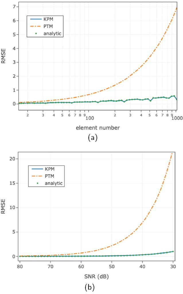
Figure 1 RMSE performance of KPM and PTM across (a) fixed SNR with various array sizes and (b) fixed array size with various SNR values. KPM shows superior scalability and noise resilience.

Figure 1 (a) shows RMSE versus array size $N$ (16 to 1024) at a fixed SNR of 40 dB. As $N$ increases, both methods exhibit rising RMSE due to more unknowns under constant noise. However, PTM shows a steeper increase, while KPM maintains RMSE below 1, with mild quasi-periodic fluctuations attributed to Kronecker structure conditioning. At $N=1024$, KPM achieves RMSE nearly 5% of PTM, demonstrating better scalability.

Figure 1 (b) shows RMSE versus SNR (30–80 dB) at fixed $N=1024$. While both methods improve with increasing SNR, KPM consistently outperforms PTM, especially below 60 dB where PTM struggles due to limited signal diversity. At 30 dB, KPM’s RMSE is only 4% of PTM’s, confirming superior noise robustness. In both cases, simulation results align with the analytical model in (12).

3.2 RMSE evaluation over DPS quantization error

This subsection validates the analytical results by isolating the effect of DPS quantization error. To remove additive noise, the SNR is set to infinity. The RMSE phase error ($\xi$) is varied from 0.1^∘ to 5^∘ in 0.1^∘ steps, with the array size fixed at $N=1024$. In this subsection, the numerical results of the KPM are compared with the analytical prediction derived in (22), which assumes a uniform array for analytical tractability.

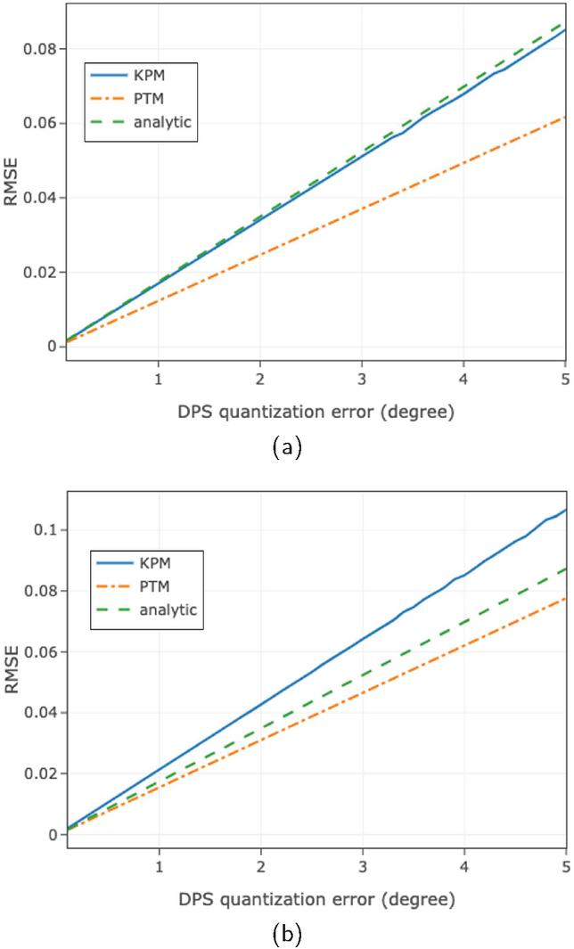
Figure 2 Average RMSE of KPM and PTM over 10,000 trials under varying DPS phase quantization error $\xi$, with SNR $\to \mathrm{\infty }$ to isolate quantization effects. (a) Uniform array and (b) non-uniform amplitudes.

We first consider a uniform array with unit amplitudes. Figure 2 (a) shows average RMSE over 10,000 trials. As expected, RMSE for both KPM and PTM increases linearly with DPS phase error. KPM exhibits slightly higher RMSE than PTM, consistent with the cumulative effect of phase errors in multi-element modulation. The KPM RMSE closely follows the analytical prediction in (22), with minor deviations due to the first-order approximation in (15). Figure 2 (b) considers amplitudes uniformly distributed between 0.5 and 1.5. Both methods show slightly higher RMSE than the uniform-amplitude case, indicating additional error from amplitude variation. Here, the prediction in (22) no longer aligns with KPM results, as it assumes $a_n=1$. In practice, unknown excitations limit the applicability of (22).

3.3 Overall RMSE analysis

Lastly, we evaluate the RMSE of KPM calibration by jointly considering array size $N$, SNR, and DPS quantization error $\xi$. While individual effects of noise and quantization were analyzed analytically, a unified closed-form expression is intractable due to nonlinear interactions. Therefore, we construct numerical error maps for practical estimation.

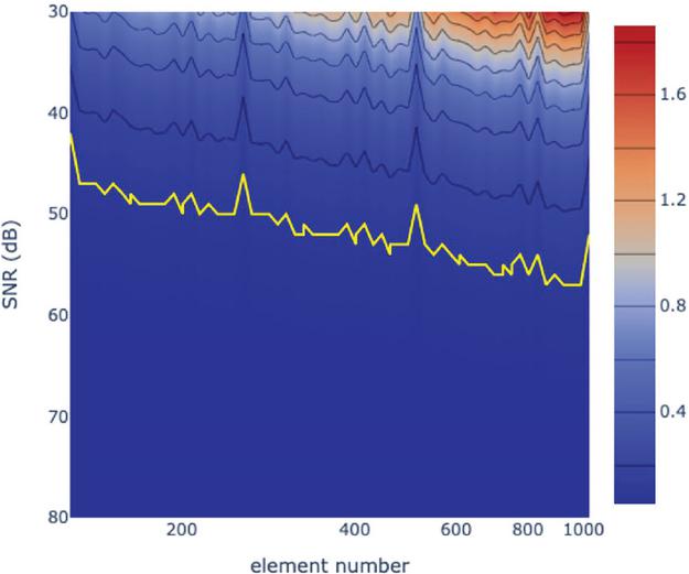
Figure 3 Contour plot of the average RMSE for the KPM calibration as a function of array size N (ranging from 128 to 1024) and SNR (ranging from 80 dB to 30 dB), with DPS phase quantization error fixed at $\xi ={2.5}^{\circ }$.

Figure 3 shows a contour plot of average RMSE (10,000 trials) versus array size ($N=128$ to $1024$) and SNR (30–80 dB), with fixed quantization error $\xi ={2.5}^{\circ }$. Along the $x$-axis (increasing $N$), RMSE trends are similar to Fig. 1 (a), driven by $N$ and $\mathrm{tr}[{\mathbf{S}}^{-1}{({\mathbf{S}}^{-1})}^H]$, but exhibit more oscillations due to phase quantization, including nulls at power-of-two sizes. Along the SNR axis, RMSE increases with decreasing SNR, as expected.

4 CONCLUSION

This paper proposes a phased array calibration method using a Kronecker product formulation with binary phase modulation to enable simultaneous multi-element excitation. We analytically prove that the resulting measurement matrix is full rank for any array size, ensuring stable recovery. Theoretical analysis includes closed-form RMSE expressions under additive noise and first-order perturbation analysis of DPS quantization effects. A numerical RMSE map is constructed to evaluate joint impacts of noise, quantization, and array size. Compared to the PTM, the proposed method achieves improved accuracy while maintaining compatibility with low-bit hardware under various array sizes and noise levels. Simulation results confirm its performance under diverse conditions. Experimental validation is planned.

References

[1] R. Hansen, Phased Array Antennas. Hoboken, NJ: John Wiley & Sons, 2009.

[2] S. Kim, H.-J. Dong, J.-W. Yu, and H. Lee, “Phased array calibration, system with high accuracy and low complexity,” Alexandria Engineering, Journal, vol. 69, pp. 759–770, 2023.

[3] J. J. Schuss, T. V. Sikina, J. E. Hilliard, P. J. Makridakis, J. Upton, J. C. Yeh, and S. M. Sparagna, “Large-scale phased array calibration,” IEEE Transactions on Antennas and Propagation, vol. 67, no. 9, pp. 5919–5933, 2019.

[4] L. Zhu, W. Ma, and R. Zhang, “Movable-antenna array enhanced, beamforming: achieving full array gain with null steering,” IEEE, Communications Letters, vol. 27, no. 12, pp. 3340–3344, 2023.

[5] A. Yaghjian, “An overview of near-field antenna measurements,” IEEE Transactions on Antennas and Propagation, vol. 34, no. 1, pp. 30–45, 1986.

[6] F. Ferrara, C. Gennarelli, and R. Guerriero, “Near-field antenna, measurement techniques,” in Handbook of Antenna, Technologies, Z. N. Chen, Ed. Singapore: Springer, pp. 2107–2163, 2016.

[7] J. Lee, E. Ferren, D. Woollen, and K. Lee, “Near-field probe used as a, diagnostic tool to locate defective elements in an array antenna,” IEEE, Transactions on Antennas and Propagation, vol. 36, no. 6, pp. 884–889, 1988.

[8] Y. Lu, L. Zhou, M. Cui, X. Du, and Y. Hu, “A method for planar phased, array calibration,” Progress In Electromagnetics Research Letters, vol. 94, pp. 19–25, 2020.

[9] Y. Lu, S. Shi, M. Cui, and L. Zhou, “Probe distance error analysis for, phased array calibration based on BTM,” Microwave and Optical, Technology Letters, vol. 64, no. 3, pp. 496–499, 2022.

[10] K. Lee, R. Chu, and S. Liu, “A performance monitoring/fault isolation, and correction system of a phased array antenna using transmission-line, signal injection with phase toggling method,” in IEEE Antennas and, Propagation Society International Symposium 1992 Digest, pp. 429–432, 1992.

[11] S. Mano and T. Katagi, “A method for measuring amplitude and phase of, each radiating element of a phased array antenna,” Electronics and, Communications in Japan (Part I: Communications), vol. 65, no. 5, pp. 58–64, 1982.

[12] W. Keizer, “Fast and accurate array calibration using a synthetic array, approach,” IEEE Transactions on Antennas and Propagation, vol. 59, no. 11, pp. 4115–4122, 2011.

[13] R. Sorace, “Phased array calibration,” IEEE Transactions on, Antennas and Propagation, vol. 49, no. 4, pp. 517–525, 2002.

[14] T. Takahashi, Y. Konishi, S. Makino, H. Ohmine, and H. Nakaguro, “Fast, measurement technique for phased array calibration,” IEEE Transactions, on Antennas and Propagation, vol. 56, no. 7, pp. 1888–1899, 2008.

[15] W. Fan, Y. Zhang, Z. Wang, and F. Zhang, “Large-scale phased array, calibration based on amplitude-only measurement with the multiround, grouped-REV method,” IEEE Transactions on Antennas and Propagation, vol. 72, no. 1, pp. 454–465, 2023.

[16] G. Hampson and A. Smolders, “A fast and accurate scheme for calibration, of active phased-array antennas,” in IEEE Antennas and Propagation, Society International Symposium. 1999 Digest. Held in conjunction with: USNC/URSI National Radio Science Meeting (Cat. No. 99CH37010), vol. 2, pp. 1040–1043, 1999.

[17] C. He, X. Liang, J. Geng, and R. Jin, “Parallel calibration method for, phased array with harmonic characteristic analysis,” IEEE Transactions, on Antennas and Propagation, vol. 62, no. 10, pp. 5029–5036, 2014.

[18] R. Long, J. Ouyang, F. Yang, W. Han, and L. Zhou, “Multi-element phased, array calibration method by solving linear equations,” IEEE, Transactions on Antennas and Propagation, vol. 65, no. 6, pp. 2931–2939, 2017.

[19] A. Graham, Kronecker Products and Matrix Calculus: With Applications. New York: Courier Dover Publications, 2018.

[20] M. Cheng, Q. Wu, C. Yu, H. Wang, and W. Hong, “A prephased, electronically steered phased array that uses very-low-resolution phase, shifters and a hybrid phasing method,” IEEE Transactions on Antennas, and Propagation, vol. 71, no. 9, pp. 7310–7322, 2023.

[21] M. Xiang, Y. Xiao, J. Deng, S. Xu, F. Yang, and H. Sun, “A low-profile, programmable 2-bit array based on a novel highly integrated element,” IEEE Transactions on Antennas and Propagation, vol. 73, no. 5, pp. 3418–3423, 2025.

[22] L. Wang and S. Zhao, “Fast reconstructed and high-quality ghost imaging, with fast Walsh-Hadamard transform,” Photonics Research, vol. 4, no. 6, pp. 240–244, 2016.

Biography

Jake W. Liu was born in Hualien, Taiwan, in 1995. He received the B.S. degree in Electrical Engineering from National Taiwan University, Taipei, Taiwan, in 2017, and the Ph.D. degree from the Graduate Institute of Communication Engineering at the same university in 2022. His research interests include antenna measurement theory, calibration of phased arrays at millimeter-wave frequencies, and computational electromagnetics. He is currently an Assistant Professor in the Department of Electronic Engineering at National Taipei University of Technology.

ACES JOURNAL, Vol. 41, No. 01, 74–80
DOI: 10.13052/2026.ACES.J.410108
© 2026 River Publishers