An Enhanced Bayesian Compressive Sensing Method of Moments for Monostatic Scattering Problems

Longhui Sun¹, Zhonggen Wang¹, and Chenlu Li²

¹School of Electrical and Information Engineering Anhui University of Science and Technology, Huainan 232001, China
15556361695@163.com, zgwang@ahu.edu.cn

²School Electrical and Information Engineering Hefei Normal University, Hefei 230061, China
chenluli@hfnu.edu.cn

Submitted On: August 19, 2025; Accepted On: November 20, 2025

ABSTRACT

In this paper, an Enhanced Bayesian Compressive Sensing method based on the Method of Moments (EBCS-MoM) is proposed to accelerate the solution of three-dimensional electromagnetic scattering problems. Unlike conventional Bayesian Compressive Sensing method based on the Method of Moments (BCS-MoM) approaches, EBCS-MoM employs a Gaussian Scale Mixture prior to model parameters and introduces Laplace or Student’s T hyperpriors to induce sparsity. To reduce the high computational cost of matrix inversion in traditional BCS-MoM, EBCS-MoM uses a surrogate function to approximate the Gaussian likelihood, allowing for an analytical posterior form. The algorithm then maximizes the marginal likelihood to construct a joint optimization problem, which is efficiently solved under the Majorization–Minimization framework using a Block Coordinate Descent method. This reduces the per-iteration complexity to $o(n^2)$. Numerical results demonstrate that the proposed method significantly accelerates computation while maintaining accuracy.

Keywords: Bayesian compressive sensing, method of moments, monostatic scattering problems.

1 INTRODUCTION

In the context of electromagnetic scattering problems, the Method of Moments (MoM) [1] is a high-precision approach that transforms integral equations into matrix equations. However, during the computational process of the MoM, the complexities in terms of memory and time are $o(N^2)$ and $o(N^3)$, respectively, which significantly restricts its practical application. To address this limitation, various fast algorithms have been proposed, including the Fast Multipole Method (FMM) [2], the Multilevel Fast Multipole Algorithm (MLFMA) [3], and the Adaptive Integral Method (AIM) [4]. Despite their advancements, these algorithms still exhibit constraints in terms of computational complexity and processing time. Consequently, more efficient algorithms have emerged, such as the Adaptive Cross Approximation (ACA) algorithm [5], the Characteristic Basis Function Method (CBFM) [6], the Hierarchically Off-Diagonal Low-Rank (HODLR) method [7], and the Compressive Sensing-based Method of Moments (CS-MoM) [8, 9]. These innovative methods demonstrate remarkable efficiency in handling electromagnetic scattering problems.

Sparse Bayesian Learning (SBL) [10, 11] is a widely popular machine learning algorithm. In [11], SBL was introduced into the framework of Compressive Sensing (CS), leading to the development of Bayesian Compressive Sensing (BCS), which has been extensively employed for sparse signal recovery. In the realm of electromagnetic scattering problems, Bayesian compressive sensing is primarily applied in two aspects. The first pertains to bistatic electromagnetic scattering models, where, in [12], BCS techniques were utilized to accelerate the solution of bistatic electromagnetic scattering problems. The second involves monostatic electromagnetic scattering models, with [13] introducing BCS into monostatic electromagnetic scattering computations. Compared to the traditional CS-MoM [9], BCS can adaptively determine the number of measurements. However, BCS based on relevance vector machines necessitates matrix inversion at each iteration, severely limiting its application to large-scale data. In recent years, several fast SBL algorithms have been proposed [14, 15, 16]. Among them, [14] introduced a greedy approach that starts from an empty model and iteratively adds and removes basis functions to reduce computational time. Leveraging this strategy, a fast Bayesian algorithm based on a Laplace prior model was developed [15] for reconstructing sparse signals and images. Subsequently, by analyzing the stable points of variational update expressions, a fast SBL algorithm based on Variational Bayesian Inference (VBI) was proposed [16]. Nevertheless, these approaches have not fundamentally resolved the computational bottleneck when handling large-scale data. Recently, the Generalized Approximate Message Passing (GAMP) [17] framework has been adopted to approximate the posterior distribution, thereby avoiding matrix inversion. However, this algorithm introduces an iterative method to replace the E-step of Expectation-Maximization (EM)-based SBL, which still fails to alleviate the computational burden associated with large-scale data. In [18], an Efficient Sparse Bayesian Learning (ESBL) Algorithm Based on Gaussian-Scale Mixtures was proposed. This algorithm exhibits a computational complexity of merely $o(n^2)$ per iteration, significantly mitigating the matrix inversion challenge encountered in the solution process of traditional SBL methods. It has been widely applied in sparse signal recovery and image reconstruction.

In this paper, we have innovatively integrated the ESBL algorithm into the CS-MoM, thereby proposing the Enhanced Bayesian Compressive Sensing method based on the Method of Moments (EBCS-MoM). The EBCS-MoM method achieves sparse modeling of parameters by incorporating a Gaussian Scale Mixture (GSM) prior within a Bayesian framework. To tackle the high computational complexity arising from the need for matrix inversion at each iteration in traditional BCS, EBCS-MoM constructs a tight lower bound for the likelihood function and introduces a surrogate function to approximate the posterior distribution, thereby transforming the joint optimization problem into a decomposable non-convex problem. Subsequently, the Block Coordinate Descent (BCD) algorithm [19] is employed within the Majorization-Minimization (MM) [20] framework to alternately optimize model parameters and hyperparameters. At each step, analytical formulas involving only vector and diagonal matrix operations are utilized, reducing the overall computational complexity to $o(n^2)$. Numerical simulation results demonstrate that, compared to the conventional Bayesian Compressive Sensing-based Method of Moments (BCS-MoM) [13], the proposed EBCS-MoM method offers faster computational efficiency while maintaining comparable accuracy.

2 THEORY

2.1 Combination of BCS and MoM

According to the MoM, the integral equation for the monostatic electric field can be transformed into the following matrix equation:

	${\text{Z}}_{N\times N}{[\text{I}({\theta }_1),\text{I}({\theta }_2),\mathrm{\dots },\text{I}({\theta }_n)]}_{N\times n}$
	$={[\text{V}({\theta }_1),\text{V}({\theta }_2),\mathrm{\dots },\text{V}({\theta }_n)]}_{N\times n},$	(1)

where Z represents the impedance matrix with dimensions of $N\times N$, ${\theta }_1,{\theta }_2\mathrm{\dots }{\theta }_n$ denote the incident angles, $\text{I}({\theta }_i)$ corresponds to the induced current for the given incident angle, and $\text{V}({\theta }_i)$ is the excitation vector associated with that incident angle. Solving equation (2.1) using the MoM for each incident angle involves a tremendous computational burden. In [13], the BCS-MoM was introduced to address this challenge.

Each row in matrix ${[\text{I}({\theta }_1),\text{I}({\theta }_2)\mathrm{\dots }\text{I}({\theta }_n)]}_{N\times n}$ represents a one-dimensional complex signal of length n. Sparse projection of these N signals yields the following expression:

${[\text{I}({\theta }_1),\text{I}({\theta }_2),\mathrm{\dots },\text{I}({\theta }_n)]}^T$	$={\mathit{\psi }}_{n\times n}\left[\begin{array}{c}y{({\theta }_1)}^T\\ y{({\theta }_2)}^T\\ \mathrm{⋮}\\ y{({\theta }_n)}^T\end{array}\right]$	(2)
	$={\mathit{\psi }}_{n\times n}{\mathit{\omega }}_{n\times N},$	(3)

where ${\mathit{\psi }}_{n\times n}$ is a sparse matrix and ${\mathit{\omega }}_{n\times N}$ is a sparse coefficient matrix. For the convenience of description, let ${[y({\theta }_1),y({\theta }_2),\mathrm{\dots },y({\theta }_n)]}^T={\mathit{\omega }}_{n\times N}$.

According to the BCS theory, we construct an independently and identically distributed Gaussian measurement matrix ${\mathit{\varphi }}_{mn}=[C_{ij}|i=1,2\mathrm{\dots }m;j=1,2\mathrm{\dots }n],m\ll n$. By transposing both sides of equation (2.1) and multiplying them simultaneously by ${\mathit{\varphi }}_{mn}$, the following expression can be obtained:

	$\left[\begin{array}{cccc}{C}_{{}_{11}}& C_{{}_{12}}& \mathrm{\cdots }& C_{{}_{1n}}\\ C_{{}_{21}}& C_{{}_{22}}& \mathrm{\cdots }& C_{{}_{2n}}\\ \mathrm{⋮}& \mathrm{⋮}& \mathrm{\ddots }& \mathrm{⋮}\\ C_{{}_{m1}}& C_{{}_{m2}}& \mathrm{\cdots }& C_{{}_{mn}}\end{array}\right]\left[\begin{array}{c}\text{I}{({\theta }_1)}^T\\ \text{I}{({\theta }_2)}^T\\ \mathrm{⋮}\\ \text{I}{({\theta }_n)}^T\end{array}\right]{\text{Z}}^T$	(4)
	$=\left[\begin{array}{cccc}{C}_{{}_{11}}& C_{{}_{12}}& \mathrm{\cdots }& C_{{}_{1n}}\\ C_{{}_{21}}& C_{{}_{22}}& \mathrm{\cdots }& C_{{}_{2n}}\\ \mathrm{⋮}& \mathrm{⋮}& \mathrm{\ddots }& \mathrm{⋮}\\ C_{{}_{m1}}& C_{{}_{m2}}& \mathrm{\cdots }& C_{{}_{mn}}\end{array}\right]\left[\begin{array}{c}\text{V}{({\theta }_1)}^T\\ \text{V}{({\theta }_2)}^T\\ \mathrm{⋮}\\ \text{V}{({\theta }_n)}^T\end{array}\right],$	(5)

which can be rewritten as:

$${\mathit{\varphi }}_{mn}\left[\begin{array}{c}\text{I}{({\theta }_1)}^T\\ \text{I}{({\theta }_2)}^T\\ \mathrm{⋮}\\ \text{I}{({\theta }_n)}^T\end{array}\right]{\text{Z}}^T={\mathit{\varphi }}_{mn}\left[\begin{array}{c}\text{V}{({\theta }_1)}^T\\ \text{V}{({\theta }_2)}^T\\ \mathrm{⋮}\\ \text{V}{({\theta }_n)}^T\end{array}\right].$$

(6)

Substituting equation (6) into equation (26) yields:

$${\mathit{\varphi }}_{mn}{\mathit{\psi }}_{n\times n}\left[\begin{array}{c}y{({\theta }_1)}^T\\ y{({\theta }_2)}^T\\ \mathrm{⋮}\\ y{({\theta }_n)}^T\end{array}\right]{\text{Z}}^T={\mathit{\varphi }}_{mn}\left[\begin{array}{c}\text{V}{({\theta }_1)}^T\\ \text{V}{({\theta }_2)}^T\\ \mathrm{⋮}\\ \text{V}{({\theta }_n)}^T\end{array}\right].$$

(7)

Let ${\mathit{\varphi }}_{mn}{[\text{V}({\theta }_1),\text{V}({\theta }_2),\mathrm{\dots },\text{V}({\theta }_n)]}^T$ be set as ${[{\text{V}}_{N\times m}^{BCS}]}^T$, where each row represents a new excitation, and there are a total of m new excitations. Similarly, let ${\mathit{\varphi }}_{mn}{\mathit{\psi }}_{n\times n}{[y({\theta }_1),y({\theta }_2),\mathrm{\dots },y({\theta }_n)]}^T$ be set as ${[{\text{I}}_{N\times m}^{BCS}]}^T$, which represents the induced current under the new excitations. Therefore, equation (27) can be rewritten as:

$${\text{ZI}}_{N\times m}^{BCS}={\text{V}}_{N\times m}^{BCS}.$$

(8)

${\text{I}}_{N\times m}^{BCS}$ can be computed using the MoM. Consequently, the following equation can be derived:

$${\text{I}}_{m\times N}^{BCS}={\mathit{\varphi }}_{m\times n}{\mathit{\psi }}_{n\times n}{\mathit{\omega }}_{n\times N},$$

(9)

where ${\text{I}}_{m\times N}^{BCS}$ is the observation matrix, which is the transpose of ${\text{I}}_{N\times m}^{BCS}$. By extracting the first-column data from matrices ${\text{I}}_{m\times N}^{BCS}$ and ${\mathit{\omega }}_{n\times N}$, then adding noise vectors $\xi$ to both sides of the equation, we derive the following Bayesian model-compliant formulation:

$${\text{I}}_1^{BCS}={\mathit{\varphi }}_{m\times n}{\mathit{\psi }}_{n\times n}{\mathit{\omega }}_1+\mathit{\xi }=\mathbf{\Phi }{\mathit{\omega }}_1+\mathit{\xi },$$

(10)

where $\mathrm{\Phi }$ serves as the sensing matrix. Within the Bayesian framework, in order to conduct inference, we need to make prior assumptions about model (30). Typically, it is assumed that ${\mathit{\omega }}_1$ and $\mathit{\xi }$ follow the following Gaussian prior models:

$p({\mathit{\omega }}_1|\mathit{\alpha })$	$={\displaystyle \prod _{i=1}^n}\mathrm{N}({\omega }_1^i|0,{\alpha }_i^{-1}),i=1,2\mathrm{\dots }n,$	(11)
$p(\mathit{\xi }|\lambda )$	$={\displaystyle \prod _{m=1}^m}\mathrm{N}({\xi }_i|0,\lambda ),i=1,2\mathrm{\dots }n,$	(12)

where $\mathit{\alpha }$ and $\lambda$ are hyperparameters of the model. Each element of $\mathit{\alpha }={[{\alpha }_1,{\alpha }_2\mathrm{\dots }{\alpha }_n]}^T$ is independent of one another, and the same holds true for each element of $\lambda ={[{\lambda }_1,{\lambda }_2\mathrm{\dots }{\lambda }_n]}^T$. Furthermore, we assume that ${\lambda }_i$ follows Gamma distributions: $p({\lambda }_i)\sim Gamma(a_0,b_0)$, where $a_0$ and $b_0$ are given parameters.

Based on the aforementioned assumptions, a multivariate Gaussian likelihood model for ${\text{I}}_1^{BCS}$ can be derived:

$p({\text{I}}_1^{BCS}|{\mathit{\omega }}_1,\lambda )={(2\pi \lambda )}^{\frac{-m}{2}}\exp \left(-{\displaystyle \frac{{\Vert {\text{I}}_1^{BCS}-\mathbf{\Phi }{\mathit{\omega }}_1\Vert }^2}{2\lambda }}\right).$

(13)

From equations (31) and (33), the marginal distribution of ${\text{I}}_1^{BCS}$ can be derived:

	$p({\text{I}}_1^{BCS}|\mathit{\alpha },\lambda )$
	$={(2\pi )}^{\frac{-m}{2}}{|D|}^{\frac{-1}{2}}\exp \left(-{\displaystyle \frac{1}{2}}{({\text{I}}_1^{BCS})}^{\mathrm{T}}{\text{D}}^{-1}{\text{I}}_1^{BCS}\right),$	(14)

where $\text{D}=\lambda \text{E}+\mathbf{\Phi }{\mathbf{A}}^{-1}{\mathrm{\Phi }}^{\mathrm{T}}$ and $\mathbf{A}=diag({\alpha }_1,{\alpha }_2\mathrm{\dots }{\alpha }_N)$. According to the Bayesian formula, the sparse posterior distribution of ${\mathit{\omega }}_1$ is given by:

	$p({\mathit{\omega }}_1|{\text{I}}_1^{BCS},\mathit{\alpha },\lambda )$
	$={\displaystyle \frac{p({\text{I}}_1^{BCS}|{\mathit{\omega }}_1,\lambda )p({\mathit{\omega }}_1|\mathit{\alpha })}{p({\text{I}}_1^{BCS}|\mathit{\alpha },\lambda )}}$
	$={(2\pi )}^{\frac{-m}{2}}{\left|{\displaystyle \sum }\right|}^{\frac{-1}{2}}$
	$\times \exp \left({\displaystyle \frac{1}{2}}{({\mathit{\omega }}_1-u)}^{\mathrm{T}}{\displaystyle {\sum }^{-1}}({\mathit{\omega }}_1-u)\right),$	(15)

where ${\mathit{\omega }}_1$ mean and covariance are:

$u$	$=\lambda {\displaystyle \sum {\mathbf{\Phi }}^{\mathrm{T}}{\text{I}}_1^{BCS}},$	(16)
${\displaystyle \sum }$	$={(\mathbf{A}+\lambda {\mathbf{\Phi }}^{\mathrm{T}}\mathbf{\Phi })}^{-1}.$	(17)

The update of hyperparameters can be regarded as a learning problem in the context of relevant vector bases. According to equation (2.1), the Type-II maximum likelihood estimates of the hyperparameters can be obtained:

${\alpha }_i^{new}$	$={\displaystyle \frac{{\gamma }_i}{u_i^2}},$	(18)
${\gamma }_i$	$=1-{\alpha }_i{\displaystyle {\sum }_{ii}},$	(19)
${(\lambda )}^{new}$	$={\displaystyle \frac{{\Vert {\text{I}}_1^{BCS}-\mathbf{\Phi }u\Vert }^2}{n-{\sum }_i{\gamma }_i}},$	(20)

where $u_i$ is the ith posterior mean weight from (36) and ${\sum }_{ii}$ is the ith diagonal element of the covariance in (37).

In order to compute the sparse vector ${\omega }_1$, this algorithm performs an iterative update process by continuously applying (38) and (40) while updating the posterior statistics of (36) and (37) until the convergence condition is satisfied. Finally, the sparse coefficient vector ${\mathit{\omega }}_1$ is approximately equal to $u$. Similarly, performing BCS-MoM restoration on each column of matrix $\mathit{\omega }$ in equation (29) allows reconstruction of the sparse coefficient matrix $\mathit{\omega }$. By substituting $\mathit{\omega }$ into equation (6), ${[\text{I}({\theta }_1),\text{I}({\theta }_2),\mathrm{\dots },\text{I}({\theta }_n)]}^T$ can be obtained. Figure 1 illustrates the algorithm flowchart of the BCS-MoM.

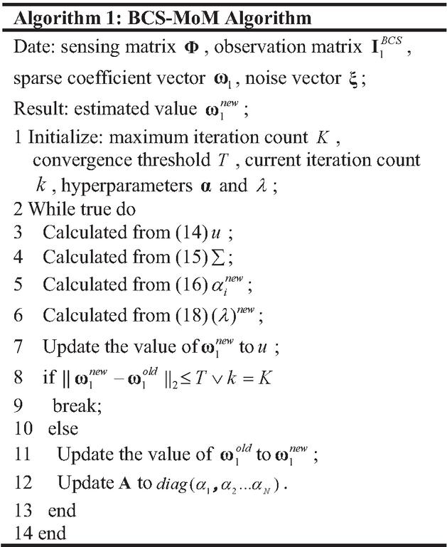
Figure 1 Flowchart of BCS-MoM algorithm.

2.2 Proposed method

To address the high computational complexity issue arising when the traditional BCS-MoM solves equation (37), this paper proposes the EBCS-MoM algorithm. By introducing a GSM prior, this algorithm constructs a lower bound function for the likelihood and employs the BCD method to optimize each parameter step by step, thereby reducing the computational load per iteration. For the detailed implementation process of EBCS, refer to [18].

In EBCS-MoM, each element of ${\mathit{\omega }}_1$ is assumed to follow a GSM prior:

$p({\omega }_1^i)$	$={\displaystyle \int p({\omega }_1^i|{\gamma }_i)p({\gamma }_i)\mathit{d}{\gamma }_i},i=1,2\mathrm{\dots }n,$	(21)
$p({\omega }_1^i|{\gamma }_i)$	$={(2\pi {\gamma }_i)}^{-\frac{1}{2}}\exp \left(-{\displaystyle \frac{{({\omega }_1^i)}^2}{2{\gamma }_i}}\right)$
	$\sim N({\theta }_i|0,{\gamma }_i),i=1,2\mathrm{\dots }n,$	(22)

where ${\gamma }_i$ is a hyperparameter that controls the sparsity of each parameter. Typically, ${\gamma }_i$ can be chosen from different distributions, such as the exponential distribution and the Gamma distribution. In this paper, we assume that ${\gamma }_i$ follows independent and identically distributed Gamma distributions: $p({\gamma }_i)\sim Gamma(c_0,d_0)$, where $c_0$ and $d_0$ are given parameters.

To avoid computing equation (33) at each iteration, EBCS introduces a lower bound of the likelihood function. By introducing auxiliary variables $\beta$ to replace the true parameter model ${\mathit{\omega }}_1$, and letting $f({\mathit{\omega }}_1)={\Vert {\text{I}}_1^{BCS}-\mathbf{\Phi }{\mathit{\omega }}_1\Vert }^2$, an upper-bound function $R({\mathit{\omega }}_1,\beta )$ is constructed as follows:

$f({\mathit{\omega }}_1)$	$\le R({\mathit{\omega }}_1,\beta )={\Vert {\text{I}}_1^{BCS}-\mathbf{\Phi }\beta \Vert }^2$
	$+2{({\mathit{\omega }}_1-\beta )}^T{\mathbf{\Phi }}^T(\mathbf{\Phi }\beta -{\text{I}}_1^{BCS})+s_0{\Vert {\mathit{\omega }}_1-\beta \Vert }^2,$	(23)

where $s_0=eig({\mathbf{\Phi }}^T\mathbf{\Phi })+\tau$ and $\tau$ is a constant. This function is equal to $f({\mathit{\omega }}_1)$ at the point where ${\mathit{\omega }}_1=\beta$.

Based on the aforementioned approximation, a surrogate likelihood function $\tilde{p}({\text{I}}_1^{BCS}|{\mathit{\omega }}_1,\lambda ,\beta )$ can be constructed:

$\tilde{p}({\text{I}}_1^{BCS}|{\mathit{\omega }}_1,\lambda ,\beta )={(2\pi \lambda )}^{\frac{-m}{2}}\exp \left(-{\displaystyle \frac{\lambda R({\mathit{\omega }}_1,\beta )}{2}}\right).$

(24)

Thus, the following equation is established:

$$p({\text{I}}_1^{BCS}|{\mathit{\omega }}_1,\lambda )=\underset{\beta }{\max }\tilde{p}({\text{I}}_1^{BCS}|{\mathit{\omega }}_1,\lambda ,\beta ).$$

(25)

By replacing $p({\text{I}}_1^{BCS}|{\mathit{\omega }}_1,\lambda )$ with its lower bound $\tilde{p}({\text{I}}_1^{BCS}|{\mathit{\omega }}_1,\lambda ,\beta )$, an approximate posterior density of ${\mathit{\omega }}_1$ can be obtained, where $\widehat{\beta }$ is fixed. According to Bayesian principles, the following approximation can be derived:

	$p({\mathit{\omega }}_1|{\text{I}}_1^{BCS},\lambda ,\gamma )$
	$\approx {\displaystyle \frac{\tilde{p}({\text{I}}_1^{BCS}|{\mathit{\omega }}_1,\lambda ,\widehat{\beta })p({\mathit{\omega }}_1|\gamma )}{\int \tilde{p}({\text{I}}_1^{BCS}|{\mathit{\omega }}_1,\lambda ,\widehat{\beta })p({\mathit{\omega }}_1|\gamma )\mathit{d}{\mathit{\omega }}_1}}\sim N(u_{{\mathit{\omega }}_1},{\displaystyle {\sum }_{{\mathit{\omega }}_1}}),$	(26)

with:

${\displaystyle {\sum }_{{\mathit{\omega }}_1}}$	$={({\mathrm{\Gamma }}^{-1}+s_0\lambda \text{E})}^{-1},\mathrm{\Gamma }=diag(\gamma ),$	(27)
$u_{{\mathit{\omega }}_1}$	$=\lambda {\displaystyle {\sum }_{{\mathit{\omega }}_1}}(s_0\widehat{\beta }-{\mathbf{\Phi }}^T\mathbf{\Phi }\widehat{\beta }+{\mathbf{\Phi }}^T{\text{I}}_1^{BCS}).$	(28)

Therefore, the point estimate of ${\mathit{\omega }}_1$ is given by:

${\widehat{\mathit{\omega }}}_1={({\mathrm{\Gamma }}_{MP}^{{}^{-1}}+s_0{\lambda }_{MP}\text{E})}^{-1}{\lambda }_{MP}(s_0\widehat{\beta }-{\mathbf{\Phi }}^T\mathbf{\Phi }\widehat{\beta }+{\mathbf{\Phi }}^T{\text{I}}_1^{BCS}),$

(29)

where ${\lambda }_{MP}$ and ${\mathrm{\Gamma }}_{MP}$ are hyperparameters to be estimated.

The subsequent critical step involves optimizing parameters $\lambda$, $\gamma$, and $\beta$. During the Type-II Maximum Likelihood Estimation process, hyperparameters can be estimated by maximizing the joint probability density function. Consequently, $\lambda$, $\gamma$, and $\beta$ are obtained through the following optimization problem:

$(\lambda ,\gamma ,\beta )$	$=\arg \underset{\lambda ,\gamma ,\beta }{\max }$
	$\times {\displaystyle \int }\tilde{p}({\text{I}}_1^{BCS}|{\mathit{\omega }}_1,\lambda ,\beta )p({\mathit{\omega }}_1|\gamma )p(\lambda )p(\gamma )d{\mathit{\omega }}_1,$	(30)

and, subsequently, the cost function L in the joint space of model parameters and hyperparameters can be obtained:

	$L({\mathit{\omega }}_1,\beta ,{\sigma }^2,\gamma )$
	$={\displaystyle \sum _{i=1}^n}\left(\ln ({\sigma }^2+s_0{\gamma }_i)+c_1\ln {\gamma }_i+{\displaystyle \frac{2d_0+{({\omega }_1^i)}^2}{{\gamma }_i}}\right)$
	$-n_1\ln {\sigma }^2+{\displaystyle \frac{R({\mathit{\omega }}_1,\beta )+2b_0}{{\sigma }^2}},$	(31)

where $n_1=n+2-m-2a_0$, $c_1=2c_0-2$, ${\sigma }^2={\lambda }^{-1}$ and $R({\mathit{\omega }}_1,\beta )$ is provided in (2.2).

EBCS decomposes the cost function into convex and concave parts, leverages the MM framework for optimization, and progressively optimizes each parameter using the BCD method. Ultimately, the update formulas for all parameters can be obtained:

$${\sum }_{{\mathit{\omega }}_1}^{(k)}={\left({\mathrm{\Gamma }}^{{(k)}^{-1}}+\frac{s_0}{{({\sigma }^2)}^k}\text{E}\right)}^{-1},$$	(32)
$${\mathit{\omega }}_1^{(k+1)}=\frac{1}{{({\sigma }^2)}^{(k)}}{\sum }_{{\mathit{\omega }}_1}^{(k)}(s_0{\beta }^{(k)}-{\mathbf{\Phi }}^T\mathbf{\Phi }{\beta }^{(k)}+{\mathbf{\Phi }}^T{\text{I}}_1^{BCS}),$$	(33)
$${\beta }^{(k+1)}={\mathit{\omega }}_1{}_{}{}^{(k+1)},$$	(34)
$${\rho }^{(k+1)}=\sum _{i=1}^n\frac{1}{{({\sigma }^2)}^{(k)}+s_0{\gamma }_{{}_i}^{(k)}},$$	(35)
$${({\sigma }^2)}^{(k+1)}=\frac{n_1+\sqrt{n_1^2+4{\rho }^{(k+1)}({\Vert {\text{I}}_1^{BCS}-\mathbf{\Phi }\beta \Vert }^2+2b_0)}}{2{\rho }^{(k+1)}},$$	(36)
$${\gamma }_{{}_i}^{(k+1)}=\sqrt{\frac{{\gamma }_i^{(k)}({({\sigma }^2)}^{(k)}+s_0{\gamma }_i^{(k)})(2d_0+{({\omega }_1^i)}^{{(k+1)}^2})}{(c_1+1)s_0{\gamma }_i^{(k)}+c_1{({\sigma }^2)}^{(k)}}},$$
$$i=1,2\mathrm{\dots }n.$$	(37)

The iteration stop threshold for EBCS is defined as:

$$\frac{\parallel {\mathit{\omega }}_1{}_{}{}^{(k+1)}-{\mathit{\omega }}_1{}_{}{}^{(k)}\parallel }{\parallel {\mathit{\omega }}_1{}_{}{}^{(k+1)}\parallel }\le \delta ,$$

(38)

where $\delta$ is defined as the threshold. The EBCS-MoM method iteratively optimizes the parameters until equation (58) is satisfied, thereby obtaining the sparse coefficient vector ${\mathit{\omega }}_1$. Similarly, performing EBCS-MoM restoration on each column of matrix $\mathit{\omega }$ in equation (29) allows reconstruction of the sparse coefficient matrix $\mathit{\omega }$. The obtained $\mathit{\omega }$ is then substituted into equation (6) to derive the original current ${[\text{I}({\theta }_1),\text{I}({\theta }_2),\mathrm{\dots },\text{I}({\theta }_n)]}^T$. Figure 2 illustrates the algorithm flowchart of the EBCS-MoM.

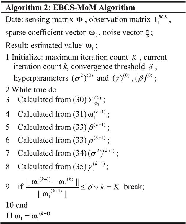
Figure 2 Flowchart of EBCS-MoM algorithm.

2.3 Computational complexity analysis

The computational complexity for impedance matrix filling and ${\text{I}}_{N\times m}^{BCS}$ is the same in both BCS-MoM and EBCS-MoM methods. Therefore, here we only compare the computational complexity of the two methods in solving equation (30).

1. BCS-MoM

The computational cost per iteration primarily centers on the inversion of the covariance matrix and the calculation of the posterior mean. The computational complexities for solving equations (36) and (37) are $o(n^2)$ and $o(n^3)$, respectively.

2. EBCS-MoM

The computational cost per iteration primarily focuses on matrix multiplication. When solving equation (52), it mainly involves the inversion of a diagonal matrix, with a computational complexity of $o(n)$. When solving equations (53), (56), and (57), the computation involves calculating ${\mathbf{\Phi }}^T\mathbf{\Phi }$, with a computational complexity of $o(n^2)$.

Therefore, the proposed method substantially decreases the computational complexity per iteration.

3 NUMERICAL RESULTS

To demonstrate the validity of the EBCS-MoM, numerical simulations of different three-dimensional conductor models are performed. Furthermore, the BCS-MoM and the GGAMP-SBL approach [17] based on the Method of Moments (GGAMP-SBL-MoM) were selected as benchmark methods for experimental comparison. To enable quantitative assessment of computational accuracy, the root-mean-square error (RMSE) metric for the monostatic radar cross section (RCS) is defined as:

$$RMSE=\sqrt{\frac{1}{N_a}\sum _{i=1}^{N_a}{|{\mathrm{RCS}}_{\mathrm{cal},i}-{\mathrm{RCS}}_{\mathrm{ref},i}|}^2},$$

(39)

where ${\mathrm{RCS}}_{\mathrm{cal},i}$ is the calculation result obtained through methods EBCS-MoM, GGAMP-SBL-MoM and BCS-MoM, ${\mathrm{RCS}}_{\mathrm{ref},i}$ is the calculation result using MoM, and $N_{\mathrm{a}}$ is the number of sampling points.

First, the monostatic scattering problem of a missile is analyzed at the angle of incidence from $\theta =0^{\circ }$ to $\theta ={180}^{\circ }$ and $\phi =0^{\circ }$, which has an incident frequency of 1.4 GHz. The target is discretized into 9178 triangles, causing 13676 unknowns.

In (6), sparse transformation is applied to ${[\text{I}({\theta }_1),\text{I}({\theta }_2),\mathrm{\dots },\text{I}({\theta }_n)]}^T$. To determine an appropriate sparse basis, Fig. 3 illustrates the errors corresponding to two commonly used sparse bases under different numbers of measurements. It can be observed that as the number of measurements increases, the errors associated with both methods decrease. Moreover, when the same number of measurements is employed, the Hermite sparse basis yields better performance compared to the Discrete Cosine Transform sparse basis (DCT). Therefore, in this paper, the Hermite sparse basis is selected.

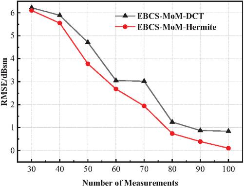
Figure 3 RMSE of BCS-MoM-DCT and EBCS-MoM-Hermite with different number of measurements.

To analyze the impact of varying iteration counts on the computational time and accuracy of two methods, Fig. 4 presents the time and accuracy results for both methods across different iteration counts. As observed from Fig. 4, the accuracy of both methods consistently improves as the number of iterations increases. Notably, when the iteration count exceeds 90, EBCS-MoM achieves higher accuracy. Furthermore, due to its lower computational complexity per iteration, EBCS-MoM requires significantly less computational time.

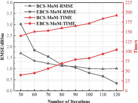
Figure 4 RMSE and solution time of BCS-MoM and EBCS-MoM with different number of iterations.

To demonstrate the advantages of the proposed method, Fig. 5 presents the computational time and error corresponding to the two methods under different numbers of measurements. As seen in Fig. 5, under varying numbers of measurements, EBCS-MoM exhibits faster computational time compared to BCS-MoM. Additionally, in comparison with the BCS-MoM method, EBCS-MoM also demonstrates certain accuracy advantages.

To demonstrate the accuracy of the proposed method, Fig. 6 presents the average current values obtained MoM and the EBCS-MoM under different incident angles, while Fig. 7 displays the RCS calculation results from three methods. As evident from Fig. 6, the current distributions computed by EBCS-MoM exhibit excellent agreement with those obtained by the MoM. From Fig. 7, it is evident that the RCS results of three methods align well with those obtained by the MoM. Moreover, EBCS-MoM exhibits superior accuracy.

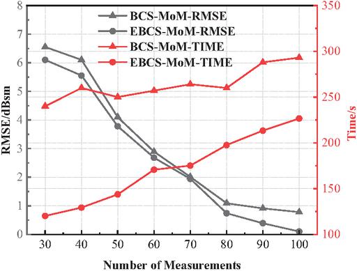
Figure 5 RMSE and solution time of BCS-MoM and EBCS-MoM with different number of measurements.

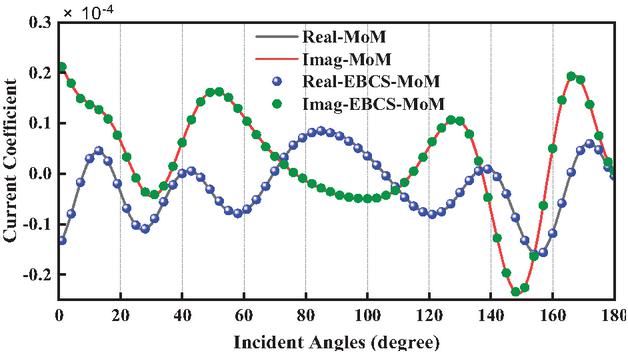
Figure 6 The average value of induced current under different incident angles.

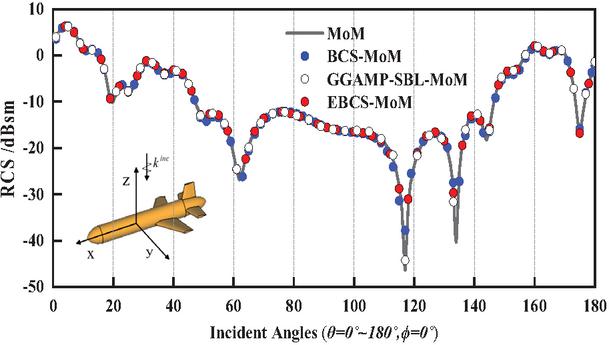
Figure 7 Monostatic RCS of missile in horizontal polarization.

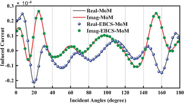
Figure 8 The average value of induced current under different incident angles.

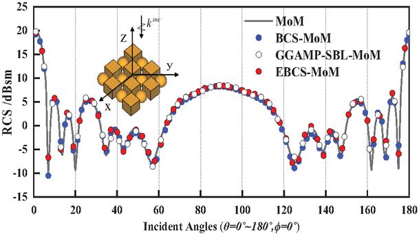
Figure 9 Monostatic RCS of the array target in horizontal polarization.

Table 1 Comparison of computation time, memory usage and RMSE

Model	Method	Unknown	Calculating	Recovery	Total	RMSE	Memory
			Observation	Induced	Time (s)	(dBsm)	(GB)
			Current	Current
			Time (s)	Time (s)
Missile	MoM	13676	–	259.98	259.98	–	2.86
	BCS-MoM		114.12	171.63	285.75	1.09	2.87
	GGAMP-SBL-MoM		114.12	112.63	226.75	0.75	2.87
	EBCS-MoM		114.12	83.28	197.40	0.61	2.87
Array Target	MoM	40824	–	2164.54	2164.54	–	25.05
	BCS-MoM		1083.25	795.30	1878.55	0.75	25.06
	GGAMP-SBL-MoM		1083.25	508.72	1591.97	0.64	25.06
	EBCS-MoM		1083.25	296.27	1379.52	0.68	25.06

Second, the scattering problem of an array target consisting of 16 PEC objects with two different shapes is analyzed. The frequency of the incident wave is set to 1.3 GHz, and the incident excitations are a set of H-polarized plane waves from $\theta =0^{\circ }$ to $\theta ={180}^{\circ }$ and $\phi =0^{\circ }$. The target is discretized into 27216 triangles, causing 40824 unknowns.

Figure 8 illustrates the average current values obtained by the MoM and EBCS-MoM under different incident angles, demonstrating excellent agreement between the current distributions computed by EBCS-MoM and those derived from the MoM. Finally, the monostatic RCS of the array target calculated by three methods are displayed in Fig. 9. Apparently, the RCS results obtained from the three methods, namely BCS-MoM, GGAMP-SBL-MoM, and EBCS-MoM, show good agreement with those calculated by the MoM.

The comparison of computation time, memory usage, and RMSE using different methods for the two models is shown in Table 1. Here, the observation current is ${\text{I}}_{m\times N}^{BCS}$. Given that the primary memory consumption stems from the storage of the impedance matrix, excitation sources, and currents, there is little difference in the memory requirements among these methods. As can be seen from Table 1, when comparing with the BCS-MoM method, the EBCS-MoM reduces the computational times 30.91% and 26.56%. Similarly, when compared with the GGAMP-SBL-MoM method, it reduces the computational times 12.94% and 13.34%. It significantly accelerates the computation while maintaining accuracy.

4 CONCLUSION

In this paper, an enhanced electromagnetic scattering algorithm is presented. The EBCS-MoM method constructs a sparse model by incorporating a GSM prior and utilizes a surrogate function to approximate the Gaussian likelihood, thereby circumventing matrix inversion. By integrating the approach of maximizing marginal likelihood, a joint optimization problem is formulated. This problem is then efficiently solved using the BCD method within the MM framework, achieving a rapid computational complexity of only $o(n^2)$ per iteration. Finally, numerical results validate the superiority of the proposed method.

ACKNOWLEDGMENT

This work was supported by the Fund of Anhui Mining Machinery and Electrical Equipment Coordination Innovation Center (Anhui University of Science and Technology) under grant No. KSJD202406.

REFERENCES

[1] R. F. Harrington, Field Computation by Moment Method. New York, NY: Macmillan, 1968.

[2] J. Dugan, T. J. Smy, and S. Gupta, “Accelerated IE-GSTC solver for large-scale metasurface field scattering problems using fast multipole method (FMM),” IEEE Trans. Antennas Propag., vol. 70, no. 10, pp. 9524–9533, Oct. 2022.

[3] H. L. Zhang, Y. X. Sha, X. Y. Guo, M. Y. Xia, and C. H. Chan, “Efficient analysis of scattering by multiple moving objects using a tailored MLFMA,” IEEE Trans. Antennas Propag., vol. 67, no. 3, pp. 2023–2027, Mar. 2019.

[4] E. Bleszynski, M. Bleszynski, and T. Jaroszewicz, “AIM: Adaptive integral method for solving large-scale electromagnetic scattering and radiation problems,” Radio Sci., vol. 31, no. 5, pp. 1225–1251, Sep. 1996.

[5] K. Zhao, M. N. Vouvakis, and J.-F. Lee, “The adaptive cross approximation algorithm for accelerated Method of Moments computations of EMC problems,” IEEE Trans. Electromagn. Compat., vol. 47, no. 4, pp. 763–773, Nov. 2005.

[6] V. V. S. Prakash and R. Mittra, “Characteristic basis function method: A new technique for efficient solution of Method of Moments matrix equations,” Microw. Opt. Technol. Lett., vol. 36, no. 2, pp. 95–100, Jan. 2003.

[7] N. Zhang, Y. Chen, Y. Ren, and J. Hu, “A modified HODLR solver based on higher order basis functions for solving electromagnetic scattering problems,” IEEE Antennas Wireless Propag. Lett., vol. 21, no. 12, pp. 2452–2456, Dec. 2022.

[8] Z. Wang, D. Dong, F. Guo, Y. Sun, W. Nie, and P. Wang, “Fast construction of measurement matrix and sensing matrix with dual adaptive cross approximation,” IEEE Antennas Wireless Propag. Lett., vol. 24, no. 1, pp. 13–17, Jan. 2025.

[9] S.-R. Chai and L.-X. Guo, “Compressive sensing for monostatic scattering from 3-D NURBS geometries,” IEEE Trans. Antennas Propag., vol. 64, no. 8, pp. 3545–3553, Aug. 2016.

[10] M. E. Tipping, “Sparse Bayesian learning and the relevance vector machine,” J. Mach. Learn. Res., vol. 1, pp. 211–244, Sep. 2001.

[11] S. Ji, Y. Xue, and L. Carin, “Bayesian compressive sensing,” IEEE Transactions on Signal Processing, vol. 56, no. 6, pp. 2346–2356, June 2008.

[12] Z. Wang, L. Sun, W. Nie, Y. Sun, D. Dong, and Y. Liu, “Rapid calculation of bistatic scattering problems based on Bayesian compressive sensing,” Electromagnetics, vol. 45, no. 4, pp. 320–333, May 2025.

[13] H.-H. Zhang, X.-W. Zhao, Z.-C. Lin, and W. E. I. Sha, “Fast monostatic scattering analysis based on Bayesian compressive sensing,” Applied Computational Electromagnetics Society (ACES) Journal, vol. 31, no. 11, pp. 1279–1285, Nov. 2016.

[14] M. E. Tipping and A. C. Faul, “Fast marginal likelihood maximization for sparse Bayesian models,” in Proc. 9th Int. Workshop Artif. Intell. Statist., pp. 1–13, 2003.

[15] S. D. Babacan, R. Molina, and A. K. Katsaggelos, “Bayesian compressive sensing using Laplace priors,” IEEE Trans. Image Process., vol. 19, no. 1, pp. 53–63, Jan. 2010.

[16] D. Shutin, T. Buchgraber, S. R. Kulkarni, and H. V. Poor, “Fast variational sparse Bayesian learning with automatic relevance determination for superimposed signals,” IEEE Trans. Signal Process., vol. 59, no. 12, pp. 6257–6261, Dec. 2011.

[17] M. Al-Shoukairi, P. Schniter, and B. D. Rao, “A GAMP-based low complexity sparse Bayesian learning algorithm,” IEEE Trans. Signal Process, vol. 66, no. 2, pp. 294–308, Jan. 2018.

[18] W. Zhou, H.-T. Zhang, and J. Wang, “An efficient sparse Bayesian learning algorithm based on Gaussian-scale mixtures,” IEEE Transactions on Neural Networks and Learning Systems, vol. 33, no. 7, pp. 3065–3078, July 2022.

[19] D. Bertsekas, Nonlinear Programming. Belmont, MA: Athena Scientific, 1999.

[20] D. R. Hunter and K. Lange, “A tutorial on MM algorithms,” Amer. Statistician, vol. 58, no. 1, pp. 30–37, Feb. 2004.

BIOGRAPHIES

Longhui Sun received the B.E. degree from Fuyang Normal University, China, in 2022. He is currently pursuing the M.S degree at Anhui University of Science and Technology. His current research interest lies in the application of Bayesian compressive sensing in electromagnetic scattering.

Zhonggen Wang received the Ph.D. degree in electromagnetic field and microwave technique from the Anhui University of China (AHU), Hefei, P. R. China, in 2014. Since 2014, he has been with the School of Electrical and Information Engineering, Anhui University of Science and Technology. His research interests include computational electromagnetics, array antennas, and reflect arrays.

Chenlu Li received the Ph.D. degree from Anhui University, China, in 2017. She is currently working at Hefei Normal University. Her research interests electromagnetic scattering analysis of targets and filtering antenna design.

ACES JOURNAL, Vol. 40, No. 12, 1160–1168
DOI: 10.13052/2025.ACES.J.401203
© 2026 River Publishers