Enhanced CPML Based on the Autoformer Network for 2D, WCS-FDTD Method

Yumeng Wu^{1, 2}, Ning Xu^{1, 2,}*, Yexin Li¹, Kuiwen Xu¹, and Juan Chen³

¹Engineering Research Center of Smart Microsensors and Microsystems, Ministry of Education, Hangzhou Dianzi University, Hangzhou 310018, China, 23040531@hdu.edu.cn, 232040214@hdu.edu.cn, kuiwenxu@hdu.edu.cn
^∗Corresponding Author
²State Key Laboratory of Millimeter Waves, Southeast University, Nanjing 210096, China, xuning_10032@hdu.edu.cn
³School of Information and Communication Engineering, Xi’an Jiaotong University, Xi’an 710049, China, chen.juan.0201@mail.xjtu.edu.cn

Submitted On: August 25, 2025; Accepted On: January 21, 2026

Abstract

This paper proposes a novel convolutional perfectly matched layer (CPML) for the weakly conditionally stable finite-difference time-domain (WCSFDTD) method. The Autoformer neural network is introduced to replace the conventional multi-layer CPML. Employing only a single-layer structure, the Auto-former-driven CPML considerably reduces both the computational domain scale and algorithmic complexity. By leveraging sequence decomposition and sparse attention mechanisms, the wave-absorption performance of this method is significantly improved. Integrated into the 2D WCS-FDTD framework, the proposed method overcomes Courant-Friedrichs-Lewy (CFL) stability constraints for FDTD intelligent absorbing boundaries, with its time step size independent of fine grid sizes in any direction. Numerical results demonstrate that the proposed method can achieve excellent wave-absorption performance with high computational efficiency, while maintaining satisfactory robustness in complex scenarios.

Keywords: Autoformer, convolutional perfectly matched layer (CPML), data-driven, weakly conditionally stable finite-difference time-domain (WCS-FDTD)..

1 INTRODUCTION

The finite-difference time-domain (FDTD) [1, 2] method, a classical technique for solving Maxwell’s equation, is widely applied in engineering scenarios including electromagnetic scattering, antenna design and photonic device simulation. However, constrained by the Courant-Friedrich-Lewy (CFL) stability condition [3, 4], its maximum time step size is strictly determined by the grid sizes in all spatial directions. Consequently, fine-scale structures in simulation objects necessitate a significantly reduced time step size, leading to a substantial increase in the computational time. To overcome this constraint, the weakly conditionally stable finite-difference time-domain (WCS-FDTD) [5, 6, 7] method has been proposed. By applying the hybrid implicit explicit technique in the fine directions, the maximum time step size of this method is only related to the coarse grid size in one direction. Therefore, the WCSFDTD method is particularly suitable for simulating electromagnetic devices that have fine structures in two directions.

In time-domain electromagnetic simulations, absorbing boundary conditions (ABCs) [8, 9, 10, 11, 12, 13, 14, 15, 16] play a crucial role in truncating computational domains. Among these, the perfectly matched layer (PML) [10] is a classical boundary condition that leverages field splitting to achieve high absorption efficiency. However, multiple layers are required to achieve effective waveabsorption, and the inherent computational complexity of field splitting further degrades its efficiency. To address these limitations, numerous PML variants have been proposed. The uniaxial PML (UPML) [12] simplifies mathematical derivations by introducing uniaxial anisotropic material parameters, while the convolutional PML (CPML) [14] achieves accelerated computation using the recursive convolution method. A further adaptation of the complex-frequency-shifted PML (CFSPML) streamlines the calculation process by incorporating multiple auxiliary variables [15]. Nevertheless, these variants still require multiple layers for effective absorption. It does not resolve the challenge of balancing performance and cost.

With the rapid advancements in computer science and hardware, recent breakthroughs in machine learning and deep learning have spurred innovations in ABCs. Yao et al. introduced a pioneering PML model based on hyperbolic tangent basis function (HTBF), which utilizes a multi-layer perceptron (MLP) to eliminate auxiliary terms [17], replace the conventional multi-layer CPML with a single layer, and thereby significantly reduce computational complexity. However, this approach suffered from error accumulation in long-term simulations. Subsequently, their team integrated a long short-term memory (LSTM) network, leveraging its temporal modeling capabilities to reduce the pile-up of errors [18]. Subsequently, further innovations demonstrated the potential of these research directions. Zhang et al. proposed a fully machine learning-driven solver that integrates LSTM model for field updating in computational domain and HTBF-PML for boundary absorption [19]. However, this model has not undergone generalization verification. Guo et al. demonstrated that the FDTD can be exactly represented by a recurrent convolutional neural network (RCNN), whose parameters were derived from the original electromagnetic equations [20]. This method requires no training, but its efficiency only improves in large-scale computations. Additionally, Feng’s research group proposed a singlelayer PML based on deep differentiable forest (DDF) to replace traditional multi-layer CPML [21]. They further applied a neural Turing machine (NTM) model incorporating deep differentiable decision trees (DDT) for effective boundary truncation in 3D microstrip line simulations [22]. They developed the gradient boosted decision trees-perfectly matched monolayer (GBDTPMM) model to tackle subsurface sensing issues [23]. Meanwhile, Ren et al. introduced a neural-networkbased CPML model by using the gated recurrent unit (GRU) [24]. However, its reliance on the multi-layer CPML structure inherently limits computational efficiency.

While the aforementioned ABCs exhibit promising absorption performance, they were primarily developed and validated within the FDTD framework. Their applicability has not been explored in the WCS-FDTD solver, which features a relaxed numerical stability criterion. This paper proposes a novel CPML method based on the Autoformer network for the 2D WCSFDTD framework. The main contributions of this paper are summarized as follows:

(1) An Autoformer-driven intelligent absorbing boundary is proposed to replace the conventional absorbing boundary. Using only a single-cell absorption layer, the Autoformer-based CPML can achieve absorption performance comparable to the conventional 6-layer CPML, while reducing computational time by 60.9%.

(2) Successful integration of the Autoformer-based CPML into the 2D WCS-FDTD framework. The time step size of this method can be set to an arbitrary value, significantly expanding the application scope of intelligent absorbing boundaries in the FDTD framework.

(3) The generalization capability is verified by modeling complex scenarios, including large computational domains, multiple excitation sources, multiple media, and fine-scale structures. Even in simulation environments far beyond the training dataset, the proposed method continues to exhibit stable and excellent wave-absorption performance.

2 FORMULATIONS

2.1 Conventional WCS-FDTD method with, CPML

It is assumed that the fine structures are contained in both the x and z directions. Fig. 1 illustrates the conventional CPML configuration for a 2D transverse magnetic (TM) case. The electromagnetic fields in this CPML region consist of three components ($H_x,H_z,E_y$). The updated equations for the 2D WCS-FDTD method with the CPML [5, 14] are given as follows:

Step 1:

$(1+{\mathrm{A}}_1+B_1)E_y^{n+\frac{1}{2}}(i,j)-A_1{E}_y^{n+\frac{1}{2}}(i+1,j)-B_1{E}_y^{n+\frac{1}{2}}(i-1,j)$
$=(1-A_1-B_1)E_y^n(i,j)+A_1{E}_y^n(i+1,j)+B_1{E}_y^n(i-1,j)-{\chi }_1\left[H_z^n(i+{\displaystyle \frac{1}{2}},j)-H_z^n(i-{\displaystyle \frac{1}{2}},j)\right]+{\beta }_1$	(1)
$H_z^{n+\frac{1}{2}}(i+{\displaystyle \frac{1}{2}},j)$
$=H_z^n(i+{\displaystyle \frac{1}{2}},j)-{\phi }_{hzx}^{n+\frac{1}{2}}(i,j)\mathrm{\Delta }t/\mu$
$-\left[E_y^{n+\frac{1}{2}}(i+1,j)-E_y^{n+\frac{1}{2}}(i+1,j)+E_y^n(i+1,j)-E_y^n(i+1,j)\right]\mathrm{\Delta }t/\left[2\mathrm{\Delta }x\mu k(i+{\displaystyle \frac{1}{2}},j)\right]$	(2)
$H_x^{n+\frac{1}{2}}(i,j)=H_x^n(i,j)$	(3)
$\{\begin{array}{cc}\hfill {\phi }_{hzx}^{n+\frac{1}{2}}(i+{\displaystyle \frac{1}{2}},j)& ={\phi }_{hzx}^n(i+{\displaystyle \frac{1}{2}},j)b_x\left(i+{\displaystyle \frac{1}{2}}\right)\hfill \\ & +\left[E_y^{\mathrm{n}+\frac{1}{2}}(i+1,j)-E_y^{\mathrm{n}+\frac{1}{2}}(i,j)+E_y^{\mathrm{n}}(i+1,j)-E_y^{\mathrm{n}}(i,j)\right]b_x\left(i+{\displaystyle \frac{1}{2}}\right)/(2\mathrm{\Delta }x)\hfill \\ \hfill {\phi }_{eyx}^{n+\frac{1}{2}}(i,j)& ={\phi }_{eyx}^n(i,j)b_x(i)+[H_z^{\mathrm{n}+\frac{1}{2}}(i+{\displaystyle \frac{1}{2}},j)\hfill \\ & -H_z^{\mathrm{n}+\frac{1}{2}}(i-{\displaystyle \frac{1}{2}},j)+H_z^{\mathrm{n}}(i+{\displaystyle \frac{1}{2}},j)-H_z^{\mathrm{n}}(i-{\displaystyle \frac{1}{2}},j)]a{}_x(i)/(2\mathrm{\Delta }x)\hfill \\ \hfill {\phi }_{eyz}^{n+\frac{1}{2}}(i,j)& ={\phi }_{eyz}^n(i,j)\hfill \\ \hfill {\phi }_{hxz}^{n+\frac{1}{2}}(i,j)& ={\phi }_{hxz}^n(i,j).\hfill \end{array}$	(4)

Step 2:

$(1+A_2+B_2)E_y^{n+1}(i,j)-A_2{E}_y^{n+1}(i,j+1)-B_2{E}_y^{n+1}(i,j-1)$
$=(1-A_2-B_2)E_y^{n+\frac{1}{2}}(i,j)+A_2{E}_y^{n+\frac{1}{2}}(i,j+1)$
$+B_2{E}_y^{n+\frac{1}{2}}(i,j-1)+{\chi }_2\left[H_x^{n+\frac{1}{2}}(i,j+{\displaystyle \frac{1}{2}})-H_x^{n+\frac{1}{2}}(i,j-{\displaystyle \frac{1}{2}})\right]+{\beta }_2$	(5)
$H_{\mathrm{x}}^{n+1}(i,j+{\displaystyle \frac{1}{2}})$
$=H_x^{n+\frac{1}{2}}(i,j+{\displaystyle \frac{1}{2}})+{\phi }_{hxz}^{n+1}(i,j+{\displaystyle \frac{1}{2}})\mathrm{\Delta }t/\mu$
$+\left[E_y^{n+1}(i,j+1)-E_y^{n+1}(i,j)+E_y^{n+\frac{1}{2}}(i,j+1)-E_y^{n+\frac{1}{2}}(i,j)\right]\mathrm{\Delta }t/\left(2\mathrm{\Delta }z\mu k_z\left(j+{\displaystyle \frac{1}{2}}\right)\right)$	(6)
$H_{\mathrm{z}}^{n+1}(i,j)=H_z^{n+\frac{1}{2}}(i,j)$	(7)
$\{\begin{array}{cc}\hfill {\phi }_{hxz}^{n+1}(i,j+{\displaystyle \frac{1}{2}})& ={\phi }_{hxz}^{n+\frac{1}{2}}(i,j+{\displaystyle \frac{1}{2}})b_z\left(j+{\displaystyle \frac{1}{2}}\right)\hfill \\ & +\left[E_y^{\mathrm{n}+1}(i,j+1)-E_y^{\mathrm{n}+1}(i,j)+E_y^{\mathrm{n}+\frac{1}{2}}(i,j+1)-E_y^{\mathrm{n}+\frac{1}{2}}(i,j)\right]a_z\left(j+{\displaystyle \frac{1}{2}}\right)/(2\mathrm{\Delta }z)\hfill \\ \hfill {\phi }_{eyz}^{n+1}(i,j)& ={\phi }_{eyz}^{n+\frac{1}{2}}(i,j)b_z(j)\hfill \\ & +\left[H_x^{\mathrm{n}+1}(i,j+{\displaystyle \frac{1}{2}})-H_x^{\mathrm{n}+1}(i,j-{\displaystyle \frac{1}{2}})+H_x^{\mathrm{n}+\frac{1}{2}}(i,j+{\displaystyle \frac{1}{2}})-H_x^{\mathrm{n}+\frac{1}{2}}(i,j-{\displaystyle \frac{1}{2}})\right]a_z(j)/(2\mathrm{\Delta }z)\hfill \\ \hfill {\phi }_{eyx}^{n+1}(i,j)& ={\phi }_{eyx}^{n+\frac{1}{2}}(i,j)\hfill \\ \hfill {\phi }_{hzx}^{n+1}(i,j)& ={\phi }_{hzx}^{n+\frac{1}{2}}(i,j).\hfill \end{array}$	(8)

The coefficients in the above equations are defined as follows:

$${\beta }_1=-\frac{\mathrm{\Delta }t}{\epsilon }{b}_x(i){\phi }_{eyx}^n(i,j)+[1/k_x(i)+a_x(i)]\frac{\mathrm{\Delta }{t}^2}{2\epsilon \mu \mathrm{\Delta }x}\left[b_x\left(i+\frac{1}{2}\right){\phi }_{hzx}^n(i+\frac{1}{2},j)-b_x\left(i-\frac{1}{2}\right){\phi }_{hzx}^n(i-\frac{1}{2},j)\right]$$

$${\beta }_2=\frac{\mathrm{\Delta }t}{\epsilon }{b}_z(j){\phi }_{eyz}^{n+\frac{1}{2}}(i,j)+[1/k_z(j)+a_z(j)]\frac{\mathrm{\Delta }{t}^2}{2\epsilon \mu \mathrm{\Delta }z}\left[b_z\left(j+\frac{1}{2}\right){\phi }_{hxz}^{n+\frac{1}{2}}(i,j+\frac{1}{2})-b_z\left(j-\frac{1}{2}\right){\phi }_{hxz}^{n+\frac{1}{2}}(i,j-\frac{1}{2})\right]$$

$$A_1=\frac{\mathrm{\Delta }{t}^2}{4\epsilon \mu \mathrm{\Delta }{x}^2}{\xi }_x(i){\xi }_x\left(i+\frac{1}{2}\right)B_1=\frac{\mathrm{\Delta }{t}^2}{4\epsilon \mu \mathrm{\Delta }{x}^2}{\xi }_x(i){\xi }_x\left(i-\frac{1}{2}\right)$$

$${\chi }_1=\frac{\mathrm{\Delta }t}{\epsilon \mathrm{\Delta }x}{\xi }_x(i){\chi }_2=\frac{\mathrm{\Delta }t}{\epsilon \mathrm{\Delta }z}{\xi }_z(j)$$

$$A_2=\frac{\mathrm{\Delta }{t}^2}{4\epsilon \mu \mathrm{\Delta }{z}^2}{\xi }_z(j){\xi }_z\left(j+\frac{1}{2}\right)B_2=\frac{\mathrm{\Delta }{t}^2}{4\epsilon \mu \mathrm{\Delta }{z}^2}{\xi }_z(j){\xi }_z\left(j+\frac{1}{2}\right)$$

$${\xi }_w(s)=\frac{1}{k_w(s)}+a_w(s)(w=x\text{or}z,s=i\text{or}j)$$

$$b_w(s)=\exp \left\{-\frac{\mathrm{\Delta }t}{{\epsilon }_0}\left[\frac{{\sigma }_w(s)}{k_w(s)}+{\alpha }_w\right]\right\}{a}_w(s)=\frac{(b_w(s)-1)}{k_w(s)({\sigma }_w(s)+k_w(s){\alpha }_w)}{\sigma }_w(s)$$

$$k_w(s)=1+(k_{\max }-1)\frac{{|w-w_0|}^m}{d^m}{\sigma }_w(s)={\sigma }_{w\max }\frac{{|w-w_0|}^m}{d^m}{\alpha }_w={\alpha }_{w\max }\frac{{|w-w_0|}^m}{d^m}$$

where $i$ and $j$ denote the indices of spatial increments, respectively, in $x$ and $z$ directions. $w_0$ is the position of interface. $d$ is the CPML thickness. ${\sigma }_{w\max }$ represents the conductivity at the outer side of CPML layers. $m$ is the order of polynomial. ${\alpha }_{w\max }$ and $k_{\max }$ are selected according to actual conditions, with their values ranging from 0 to 0.05, and 5 to 10, respectively. $\epsilon$ is the permittivity, and $\mu$ is the permeability.

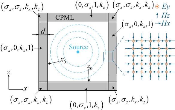
Figure 1 Conventional CPML method.

Different from the explicit update in FDTD algorithm, the WCS-FDTD method divides one iteration into two sub-time steps. The update of the electric field component $E_y^{n+\frac{1}{2}}$ in Step 1 involves the magnetic field $H_z^{n+\frac{1}{2}}$ at the same time instance, and the update of the electric field $E_y^{n+1}$ in Step 2 requires the concurrent magnetic field component $H_x^{n+1}$. Both updates necessitate implicit difference calculations. To complete one iteration, it is necessary to solve 2 implicit equations and 6 explicit equations. By adopting the implicit method in the $x$ and $z$ directions, the time step size of the WCS-FDTD method is independent of the grid size along these coordinates. Hence, an arbitrary time step size can be employed in the 2D WCS-FDTD method.

2.2 Autoformer-driven CPML

As a deep learning network, Autoformer demonstrates excellent efficiency and accuracy in time series forecasting [25, 26]. To balance between prediction accuracy and computational speed in CPML, a compact architecture is used in this paper. Fig. 2 shows its detailed structure. It includes two key modules: $(i)$ a time series decomposition module, which uses two 1D convolutional layers with different kernel sizes to decompose the input sequence into a long-term trend and a short-term seasonal component, enabling the model to capture distinct feature patterns. $(ii)$ an auto-correlation module, which integrates sparse mechanisms and multi-head mechanisms. The sparse mechanism extracts highscore components along the last dimension of the score matrix, facilitating the capture of core sequence features and preventing overfitting. The multi-head mechanism enables parallel output from multiple autocorrelation layers, which are then mapped to the model’s dimension via a linear layer to capture sequence information from multiple perspectives. Subsequently, the results are normalized via layer normalization and pass through an attention pooling module for feature refinement. In the attention pooling layer, the attention score matrix is computed by passing the module input through a linear layer. Following this scheme, the matrix is normalized by a SoftMax function and then multiplied with the input sequence. The resulting weighted sequence is finally summed along the last dimension to produce the output.

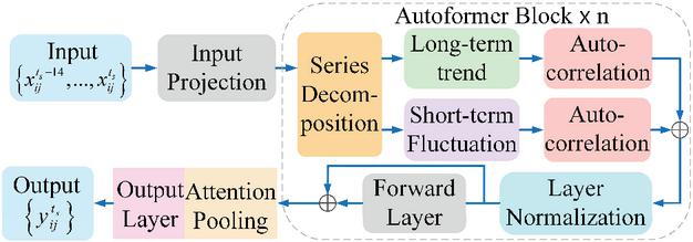
Figure 2 Autoformer model framework.

During the data acquisition phase, let $x_{ij}^t$ denote the input electromagnetic field components at the current time $t$, where $i$ and $j$ represent the spatial indices of the grid position. Let $y_{ij}^{t+1}$ denote the output electromagnetic field components at the next time step $t+1$. For each data sample, it consists of an input sequence $X^t=\{x^{t-14},\mathrm{\dots },x^t\}$ of length 15, which comprises electromagnetic field components from 15 consecutive time steps, and an output label $Y^{t+1}=\{y^{t+1}\}$ representing the field data at the subsequent time step $t+1$.

As depicted in Fig. 3, different data collection strategies are applied to the cells at the corners and edges of the computational boundary. (a) edge cells: data are gathered from a cell on the CPML boundary and its directly adjacent neighbor inside the computational domain; (b) corner cells: data are gathered from the CPML cell and a diagonally adjacent neighbor. To balance prediction accuracy and computational efficiency, the input features are composed of the electromagnetic field components from three adjacent cells, totaling 9 features per time step. The output feature set is defined as the three field components of one boundary cell, which is highlighted in red in Fig. 3. In the conventional CPML implementations for WCS-FDTD method, the calculation for one discrete time step is performed using two sub-procedures. First, the electromagnetic fields at the intermediate time step $n+1/2$ are calculated using the values at time step $n$. Subsequently, the fields at time step $n+1$ are derived from those at $n+1/2$. While, in the proposed Autoformer-driven CPML, the electromagnetic field values at the intermediate time step $n+1/2$ are not required. Only the field values at time steps $n$ and $n+1$ are collected. The specific input and output data at one time step are as follows: In edge cells:

$\{\begin{array}{cc}\hfill x_{ij}^t=[& H_z^t(i-3/2,j+1),H_x^t(i-2,j+1/2),\hfill \\ & E_y^t(i-2,j+1),H_z^t(i-1/2,j+1),\hfill \\ & H_x^t(i-1,j+1/2),E_y^t(i-1,j+1),\hfill \\ & H_z^t(i+1/2,j+1),H_x^t(i,j+1/2),\hfill \\ & E_y^t(i,j+1)]\hfill \\ \hfill y_{ij}^{t+1}=[& H_z^t(i+1/2,j+1),H_x^t(i,j+1/2),\hfill \\ & E_y^t(i,j+1)].\hfill \end{array}$

(9)

In corner cells:

$\{\begin{array}{cc}\hfill x_{ij}^t=[& H_z^{t+1}(i-3/2,j+3),H_x^{t+1}(i-2,j+5/2),\hfill \\ & E_y^{t+1}(i-2,j+3),H_z^{t+1}(i-1/2,j+2),\hfill \\ & H_x^{t+1}(i-1,j+3/2),E_y^{t+1}(i-1,j+2),\hfill \\ & H_z^{t+1}(i+1/2,j+1),H_x^{t+1}(i,j+1/2),\hfill \\ & E_y^{t+1}(i,j+1)]\hfill \\ \hfill y_{ij}^{t+1}=[& H_z^{t+1}(i+1/2,j+1),H_x^{t+1}(i,j+1/2),\hfill \\ & E_y^{t+1}(i,j+1)].\hfill \end{array}$

(10)

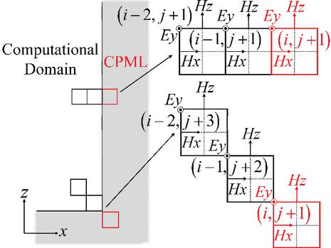
Figure 3 Data acquisition mechanism for Autoformer-driven CPML.

To ensure the model’s generalization capability, multiple electromagnetic simulation scenarios were selected for training data collection, encompassing single-point source, 9-point source, and 13-point source configurations. Each data sample captures 300 time steps of electromagnetic field evolution. Considering the implicit computation, a column-stacking approach was adopted for data acquisition, which enhances storage and update efficiency while remaining applicable to the FDTD framework. The final training dataset comprises input samples with dimensions (106392, 15, 9) and output labels with dimensions (106392, 1, 3), where 106392 denotes the total number of samples, 15 is the sequence length of the input data, 9 is the number of input features, 1 is the sequence length of the output label, and 3 is the number of output features. All training and evaluation processes were implemented using the PyTorch deep learning framework on a system equipped with an AMD Ryzen 9 9950X CPU and an NVIDIA GeForce RTX 4080 Super GPU. The training of this model takes 797 s.

Table 1 Ablation study for the important components

Method	${\mathit{H}}_{\mathit{x}}$ Error $\mathbf{\downarrow }$	${\mathit{H}}_{\mathit{z}}$ Error $\mathbf{\downarrow }$	${\mathit{E}}_{\mathit{y}}$ Error $\mathbf{\downarrow }$	MSE$\mathbf{\downarrow }$	Time(s)	Params
Autoformer	3.94e-05	3.80e-05	5.09e-05	4.28e-5	416.56	35640
w/o Sparse Mechanism	3.78e-05	3.87e-05	4.38e-05	4.01e-5	472.83	35640
w/o Series Decomposition	1.15e-04	3.32e-04	1.97e-04	2.15e-4	369.16	18036
w/o Multi-head Mechanism	3.16e-04	2.13e-04	2.38e-04	2.56e-4	327.61	21006
w/o Attention Polling	4.41e-05	4.75e-05	6.38e-05	5.18e-5	399.45	35612

2.3 Ablation study and parameter selection

To evaluate the contribution of each component in the proposed Autoformer architecture, an ablation study was performed by assessing the impact of removing the sparse attention, sequence decomposition, multi-head mechanism, and attention pooling modules. Table 1 summarizes the corresponding performance changes in terms of component errors ($H_x,H_z,E_y$), mean squared error (MSE), inference times, and the number of parameters.

The experimental results indicate that removing either the series decomposition module or the multi-head mechanism leads to significant performance degradation, with the MSE increasing by approximately one order of magnitude. These results highlight the crucial role both components play in enhancing feature representation and improving predictive accuracy. Replacing the sparse attention with a full attention mechanism reduces the overall MSE to 4.01e-4 but markedly increases the inference time, suggesting that sparsification effectively balances computational efficiency and model representational capacity. Furthermore, removing the attention pooling module reduces the parameter count but also leads to notable increases in all error metrics, confirming its essential role in maintaining prediction accuracy.

In neural network construction and training, parameter design is important. The specific parameter configurations are as follows:

(1) Convolution kernel: In the series decomposition, a kernel size of 3 is employed to extract short-term fluctuations, while a kernel size of 9 is used for extracting long-term trends.

(2) Hidden layer size: An excessively large size may induce overfitting and compromise computational efficiency, whereas an insufficient size fails to adequately capture the nonlinear input-output relationship. After balancing computational efficiency with model capacity, the hidden layer size is set to 27.

(3) Sparse mechanism factor: A factor of 0.34 is selected to accelerate both model training and inference while simultaneously mitigating overfitting.

(4) Number of heads: Five heads are configured to enable comprehensive extraction of data features across multiple dimensions.

(5) Training parameters: The network is trained using the AdamW optimizer with an initial learning rate of 0.003. This pairing represents a standard, well-established choice for training deep neural networks, as it delivers stable convergence and effective regularization.

2.4 Integration of autoformer-driven CPML with WCS-FDTD

Based on the trained Autoformer network, $\{y_{ij}^{t+1}\}$ can be predicted by $\{x_{ij}^{t-14},\mathrm{\dots },x_{ij}^t\}$ and the electromagnetic fields on the CPML interface at $t+1$ can be further obtained. Then, using $\{y_{ij}^{t+1}\}$, the electromagnetic fields in the object domain at $t+1$ can be obtained via the standard WCS-FDTD process. Meanwhile, the field values within both the CPML layer and its adjacent region in the object domain are stored for use as the input features at $t+2$. By repeating this process, the Autoformer-driven CPML can replace the conventional multi-layer CPML and be integrated into the WCS-FDTD framework. The specific algorithm is shown as follows:

Algorithm: Autoformer-driven CPML on
WCSFDTD framework
Data Collection and Training
(1)	Collect the dataset $\{x_{ij}^{t_{s-14}},\mathrm{\dots },x_{ij}^{t_s}\}$ and $\{y_{ij}^{t_s}\}$ in a columnar fashion.
(2)	Train the Autoformer-driven CPML using the collected dataset.
Network Prediction Substitution
Initialization $\mathbf{(}\mathit{k}\mathbf{<}\mathbf{15})$:
(1)	Initialize the electromagnetic field values at each time step using WCS-FDTD method.
(2)	Collect data at each time step and stack them in the format required for the model input.
$\mathit{k}$th Iteration $\mathbf{(}\mathit{k}\mathbf{\ge }\mathbf{15}\mathbf{)}$:
(3)	Update input sequence $X^t=\{x^{t-14},\mathrm{\dots },x^t\}$ using a sliding window.
(4)	Predict boundary fields $\{y^{t+1}\}$ by using Autoformer model.
(5)	Update the electromagnetic fields on the first CPML layer with $\{y^{t+1}\}$.
(6)	Update the electromagnetic fields in the object domain at $t+1$ using WCS-FDTD method.

3 NUMERICAL EXAMPLES

To evaluate the performance of the proposed method, three distinct scenarios are simulated. Case A is primarily used to validate the wave-absorption performance of Autoformer-driven CPML, whereas cases B and C are designed to assess its generalization capability across various complex scenarios.

3.1 Single point source

To validate the wave-absorption performance of this Autoformer model, the propagation process of a single source under identical environmental parameters to those in the training dataset is modeled. As illustrated in Fig. 4, the computational domain is $60\mathrm{mm}\times 60\mathrm{mm}$, with a grid size of $2\mathrm{mm}\times 2\mathrm{mm}$ and a time step size of 2 ps. A sinusoidal point source is located at the center of the computational domain. It should be noted that the conventional CPML requires a multi-layer structure to achieve satisfactory wave-absorption, whereas the proposed Autoformer model only needs one layer.

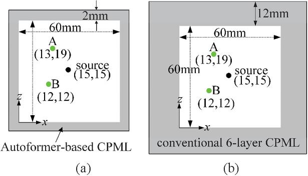
Figure 4 Profile of a single point source: (a) Autoformer-driven CPML and (b) conventional 6-layer CPML.

To evaluate the performance of the proposed method, the relative error is defined by the following formula:

$$\mathit{Error}{(t)}_{\mathrm{dB}}=20\times {\log }_{10}\frac{|E_y(t)-E_y^{\mathrm{ref}}(t)|}{|E_y^{\mathrm{ref},\max }(t)|}$$

(11)

where $E_y(t)$ is the predicted electric field, $E_y^{\text{ref}}(t)$ is the boundary-reflection-free reference electric field, and $E_y^{\text{ref,max}}(t)$ is the maximum value of the reference electric field.

Figure 5 shows the relative errors of various methods at observation points A and B during the time intervals from $t=600\mathrm{ps}$ to $t=1000\mathrm{ps}$, and from $t=3600\mathrm{ps}$ to $t=4000\mathrm{ps}$. For point A, the conventional 1-layer CPML and 6-layer CPML show $-$11 dB and $-$37 dB errors, respectively. For comparison, the HTBF-based PML and LSTM-based PML, which are originally developed for the 2D FDTD method, were migrated into the WCS-FDTD framework. The input data structure was reshaped to $(15,9)$ for the LSTM model and $(1,9)$ for the HTBF model, with the output data structure being $(1,3)$ for both. To achieve optimal performance, the hidden layer sizes were set to 27 and 36 for the HTBF and LSTM models, respectively. The maximum errors of the HTBF model and LSTM model are $-$31 dB and 34 dB, respectively. Meanwhile, the maximum error of the Autoformer-driven CPML is only $-$40 dB, which is lower than that of both the conventional CPMLs and other machine-learning-driven CPMLs. For point B, the maximum relative errors of conventional 1-layer CPML, 6-layer CPML, HTBF model, LSTM model and Autoformer model are $-$9 dB, $-$35 dB, $-$28 dB, $-$32 dB and $-$40 dB, respectively. The Autoformer-driven CPML achieves the best wave-absorption performance.

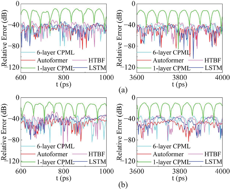
Figure 5 Error comparison among five methods: (a) relative error at point A and (b) relative error at point B.

Since the algorithm operates in the time domain, a long-term simulation was performed to validate its stability. As shown in Fig. 6, the electric field waveform at observation point A remains stable and consistent with the conventional 120-layer CPML, even after 100,000 time steps. This result confirms that the proposed method retains high predictive stability in prolonged simulations.

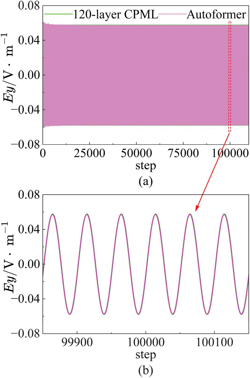
Figure 6 Long-term stability and accuracy verification of 100,000 time steps: (a) long-term waveform diagram and (b) detailed waveform comparisons at the late stage.

To further evaluate the performance of the proposed method, Fig. 7 compares the average relative errors of these five methods across the entire computational domain. The conventional 1-layer CPML shows an average error of $-$13 dB, indicating ineffective waveabsorption. Moreover, the average errors for other methods are respectively $-$37 dB for the conventional 6-layer CPML, $-$30 dB for the HTBF model, $-$32 dB for the LSTM model and $-$39 dB for the Autoformer model. The proposed method achieves the lowest absorption error. Compared to the conventional 6-layer CPML, the proposed method’s absorption effect improves by 2 dB. Besides, it demonstrates 9 dB and 7 dB improvements over the HTBF and LSTM models, respectively.

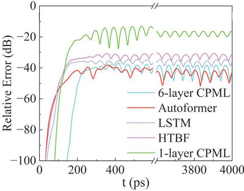
Figure 7 The average relative error over the entire computational domain.

Table 2 records the single-step computational time for the above five methods. Completing one-step simulation, the conventional 1-layer CPML and 6-layer CPML take 0.00694 s and 0.01187 s, respectively, whereas the Autoformer-driven CPML only spends 0.00464 s. Obviously, the Autoformer-driven CPML achieves a wave-absorbing effect comparable to that of the conventional 6-layer CPML, however, its computational time is reduced by 60.9%. Unfortunately, the computational cost of the Autoformer model is higher than that of HTBF model (0.00268 s) and LSTM model (0.00305 s).

Table 2 Comparison of single-step simulation time between deep learning networks and conventional CPML methods for Case A

Method	1-layer	6-layer	HTBF	LSTM	Autoformer
	CPML	CPML
Average
Time (s)	0.00694	0.01187	0.00268	0.00305	0.00464

To further assess the computational efficiency of the proposed method, Fig. 8 presents the average single-step computational cost across different computational scales. Both the Autoformer-driven CPML and LSTM model are faster than the conventional CPML, and these performance advantages become increasingly significant as the grid scale increases. This is because the conventional CPML needs to calculate convolution terms grid by grid, while the deep learning driven CPMLs only predict the electromagnetic field values on the boundaries. When comparing the LSTM model and the Autoformer model, the LSTM model performs serial operations in the time dimension, whereas the Autoformer model incorporates a GPU-accelerated parallel architecture. This powerful parallel computing capability greatly saves computational time in large-scale computations. As shown in Fig. 8, although the Autoformer model has a higher computational cost than the LSTM model, the performance gap between them is gradually narrowing as the computational scale increases.

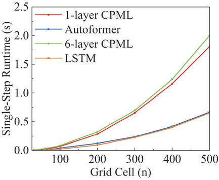
Figure 8 Single-step simulation time of various methods under different computational scales.

3.2 Large domain with multiple point sources

To evaluate the generalization ability of the proposed method, a model with a large computational domain containing multiple point sources is established. Different from the training set, the computational domain of this simulation model is expanded to $140\mathrm{mm}\times 140\mathrm{mm}$. As shown in Fig. 9, one point source is placed at the center of the computational domain, and the other four point sources exactly form a square. Other simulation parameters are the same as those in single source example.

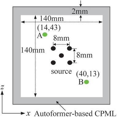
Figure 9 Large computational domain with multiple point sources.

Figures 10 and 11 compare the relative errors of different methods. As shown in Fig. 10, the maximum relative error of the conventional 1-layer CPML reaches $-$7 dB at point A and $-$8 dB at point B, while the conventional 6-layer CPML reaches $-$35 dB at point A and $-$36 dB at point B. In contrast, the Autoformer-driven CPML exhibits the lowest errors of $-$38 dB at point A and $-$37 dB at point B. The LSTM model yields $-$30 dB and $-$32 dB at point A and B, respectively. However, in long-term simulation, the error of the HTBF model suffers from gradual accumulation, resulting in higher errors of $-$13 dB at point A and $-$11 dB at point B.

In addition, the average relative errors over the entire computational domain are shown in Fig. 11. The average error of the conventional 1-layer CPML is $-$13 dB. The HTBF model, due to error accumulation in long-term simulations, also has a high average error of 13 dB. Notably, the Autoformer-driven CPML achieves an average relative error of $-$38 dB, which is superior to the LSTM model ($-$33 dB) and the conventional 6-layer CPML ($-$37 dB).

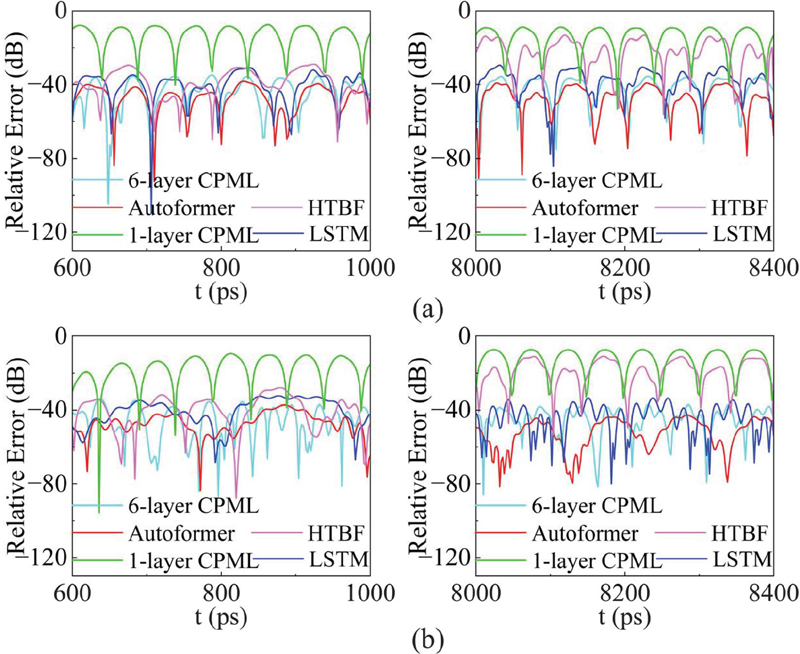
Figure 10 Relative error of five excitation sources: (a) relative error at point A and (b) relative error at point B.

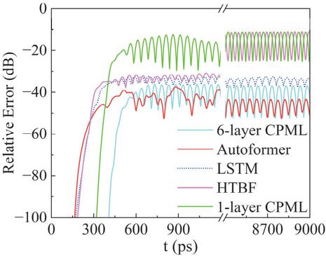
Figure 11 The average relative error over the entire computational domain.

Furthermore, Table 3 lists the single-step simulation time for each method. For a single-step computation, the conventional 1-layer CPML and conventional 6-layer CPML take 0.03508 s and 0.04565 s, respectively, whereas the LSTM model and Autoformer-driven CPML only require 0.01535 s and 0.02752 s. From the above analysis, it can be observed that when simulating scenarios more complex than those in the training set, the proposed Autoformer-driven CPML maintains high wave-absorption effectiveness with low computational cost. This preliminarily demonstrates the generalization ability of this method.

Table 3 Comparison of single-step simulation time between deep learning networks and conventional CPML methods for Case B

Method	1-layer	6-layer	LSTM	Autoformer
	CPML	CPML
Average
Time (s)	0.03508	0.04565	0.01535	0.02752

3.3 Multi-scale and multi-medium structure

To further evaluate the generalization ability of the proposed method, a complex scenario involving fine metal structures is established. As shown in Fig. 12, the key environmental parameters differing from the training set are summarized as follows:

(1) Multi-material environment: Two metallic blocks are introduced to create a multi-material environment, one of which contains fine structural features.

(2) Multi-scale structures: Fine meshes with a minimum grid size of $\mathrm{\Delta }{x}_{\min }=\mathrm{\Delta }{z}_{\min }=0.2\mathrm{mm}$ are adopted in both the $X$ and $Z$ directions.

(3) Large time step size: A large time step size of 4 ps is adopted. This value exceeds the limit of the CFL stability condition in the FDTD framework and the time step size used in the training set.

(4) Multiple excitation sources: Five point sources are used as the excitation sources for the simulation model.

(5) Large computational domain: The computational domain is expanded to $140\mathrm{mm}\times 140\mathrm{mm}$.

All other simulation parameters remain the same as those in the training set cases.

Figure 13 presents the error analysis of the specified observation points. The HTBF model initially exhibits satisfactory wave-absorption performance. However, its error accumulates over time, resulting in a decline in performance, with maximum relative errors reaching 10 dB at point A and $-$11 dB at point B. In contrast, other methods maintain stability. The maximum relative errors of the conventional 1-layer CPML, 6-layer CPML, and the LSTM model at point A are $-9\mathrm{dB},-35$ dB, and $-$28 dB, and at point B are $-8\mathrm{dB},-34\mathrm{dB}$, and 25 dB, respectively. The Autoformer-driven CPML achieves the lowest errors of $-$41 dB at point A and $-$38 dB at point B, demonstrating excellent wave-absorption performance.

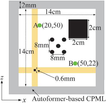
Figure 12 A complex simulation scenario with five excitation sources, a large computational domain, and multiple metal blocks.

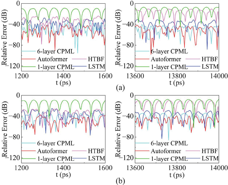
Figure 13 The relative errors of the five methods: (a) relative error at point A and (b) relative error at point B.

Subsequently, the average relative errors of these methods are discussed. As shown in Fig. 14, the HTBF model gradually accumulates errors after 9000 ps, eventually reaching $-$13 dB. The error of the LSTM model increases to $-$27 dB, while the Autoformer model maintains a lower error of $-$38 dB, comparable to that of the conventional 6-layer CPML ($-$36 dB). It is evident that the proposed model exhibits excellent wave-absorption performance with a larger time step size. Notably, the time step size of 4 ps breaks through the CFL limit of the FDTD framework, enabling a significant expansion of the application range for intelligent absorption boundaries.

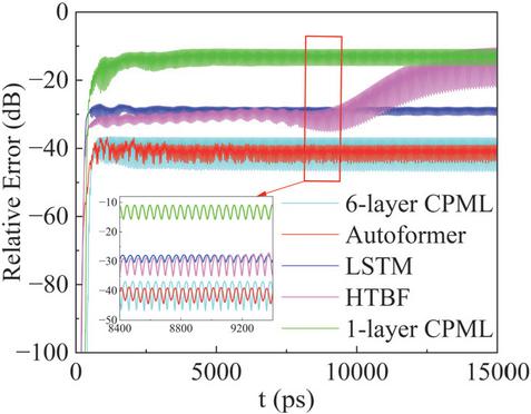
Figure 14 The average relative error over the entire computational domain.

In addition, as shown in Table 4, for single-step simulation, the Autoformer-driven CPML takes 0.02537 s, which is slightly longer than the 0.01875 s required by the LSTM model, but significantly shorter than the 0.04857 s of the conventional 1-layer CPML and 0.06307 s of the conventional 6-layer CPML. Obviously, compared with conventional CPMLs, the proposed method achieves comparable wave-absorption performance to the conventional 6-layer CPML while reducing computation time by 59.79%. Relative to the LSTM model, it exhibits a 11 dB improvement in wave-absorption performance. Furthermore, as the computational scale increases, the additional time cost decreases from 52.13 % to 35.25%, indicating that the efficiency gap diminishes at larger scales. From the above analysis, it can be concluded that even in scenarios considerably more complex than the training set, the proposed method maintains excellent wave-absorption performance and fast simulation, which validates the robustness of the proposed method. This robustness holds for electromagnetic environments with multiple media, multiple sources, multiple scales, large time step sizes, and large computational domains, underscoring the method’s potential as a practical tool for engineering applications.

Table 4 Comparison of single-step simulation time between deep learning networks and conventional CPML methods for Case C

Method	1-layer	6-layer	LSTM	Autoformer
	CPML	CPML
Average
Time (s)	0.04857	0.06307	0.01875	0.02537

4 CONCLUSION

This paper proposes an Autoformer-driven CPML for the WCS-FDTD framework to improve the efficiency of open-region simulations. The Autoformer-based CPML employs a single-layer structure to replace the conventional multi-layer CPML, significantly reducing both the computational domain scale and algorithmic complexity. Compared to the conventional CPMLs and other deep-learning-driven PML approaches, this new model provides superior wave-absorption effectiveness and high computational efficiency. Integrated into the WCS-FDTD framework, this method overcomes CFL stability constraints, substantially expanding the modeling scope of intelligent absorption boundaries. Furthermore, the proposed method exhibits satisfactory wave-absorption performance and excellent generalization capability in complex scenarios involving multi-material environments, multi-source excitations, multi-scale structures, large computational domains, and extended time step sizes. Moreover, by adjusting the sampling strategy and modifying the input-output dimensions, this proposed method can be extended to 3D scenes, which constitutes a key direction for our future work.

ACKNOWLEDGMENT

This work was supported in part by the State Key Laboratory of Millimeter Waves under Grant K202518 and in part by the Zhejiang Provincial Natural Science Foundation of China under Grant LQN25F010010 and LQN25F010011.

References

[1] A. Taflove and S. C. Hagness, Computational Electrodynamics: The Finite-Difference Time-Domain Method, 3rd ed. Boston, MA, USA: Artech House, 2005.

[2] W. Sun, “Automatic and efficient surface FDTD mesh generation for analysis of EM scattering and radiation,” Applied Computational Electromagnetics Society (ACES) Journal, vol. 9, no. 2, pp. 162–169, July 2022.

[3] K. S. Yee, “Numerical solution of initial boundary value problems involving Maxwell’s equations in isotropic media,” IEEE Trans. Antennas Propagat., vol. AP-14, pp. 302–307, 1966.

[4] R. Courant, K. Friedrichs, and H. Lewy, “On the partial difference equations of mathematical physics,” IBM J. Res. Dev., vol. 11, no. 2, pp. 215–234, Mar. 1967.

[5] J. Chen and J. Wang, “A novel WCS-FDTD method with weakly conditional stability,” IEEE Trans. Electromagn. Compat., vol. 49, no. 2, pp. 419–426, 2007.

[6] J. Chen, “Improved weakly conditionally stable finite-difference time-domain method,” Applied Computational Electromagnetics Society (ACES) Journal, vol. 27, no. 5, pp. 413–419, Feb. 2022.

[7] J. Chen and H. Mai, “A review of weakly conditional stable finite-difference time-domain method for modeling electromagnetic problems with fine structures,” Int. J. Numer. Model.: Electron. Networks, Devices Fields, vol. 31, no. 5, p. e2341, 2018.

[8] G. Mur, “Absorbing boundary conditions for the finite-difference approximation of the time-domain electromagnetic-field equations,” IEEE Trans. Electromagn. Compat., vol. EMC-23, no. 4, pp. 377–382, 1981.

[9] B. Engquist and A. Majda, “Absorbing boundary conditions for the numerical simulation of waves,” Math. Comput., vol. 31, no. 139, pp. 629–651, 1977.

[10] J.-P. Berenger, “A perfectly matched layer for the absorption of electromagnetic waves,” J. Comput. Phys., vol. 114, no. 2, pp. 185–200, 1994.

[11] J.-P. Berenger, “Perfectly matched layer for the FDTD solution of wave-structure interaction problems,” IEEE Trans. Antennas Propag., vol. 44, no. 1, pp. 110–117, 1996.

[12] A. P. Zhao, “Uniaxial perfectly matched layer media for an unconditionally stable 3-D ADI-FD-TD method,” IEEE Microw. Wireless Compon. Lett., vol. 12, no. 12, pp. 497–499, 2002.

[13] L. Bernard, R. R. Torrado, and L. Pichon, “Efficient implementation of the UPML in the generalized finite-difference time-domain method,” IEEE Trans. Magn., vol. 46, no. 8, pp. 3492–3495, 2010.

[14] J. A. Roden and S. D. Gedney, “Convolutional PML (CPML): An efficient FDTD implementation of the CFS-PML for arbitrary media,” Microw. Opt. Technol. Lett., vol. 27, no. 5, pp. 334–339, 2000.

[15] S. D. Gedney, “An auxiliary differential equation formulation for the complex-frequency shifted PML,” IEEE Trans. Antennas Propag., vol. 58, no. 3, pp. 838–847, 2010.

[16] R. Martin and D. Komatitsch, “An unsplit convolutional perfectly matched layer technique improved at grazing incidence for the viscoelastic wave equation,” Geophys. J. Int., vol. 179, no. 1, pp. 333–344, 2009.

[17] H. M. Yao and L. Jiang, “Machine-learning-based PML for the FDTD method,” IEEE Antennas Wireless Propag. Lett., vol. 18, no. 1, pp. 192–196, 2018.

[18] H. M. Yao and L. Jiang, “Enhanced PML based on the long short-term memory network for the FDTD method,” IEEE Access, vol. 8, pp. 21028–21035, 2020.

[19] H. H. Zhang, H. M. Yao, L. Jiang, and M. Ng, “Deep long short-term memory networks-based solving method for the FDTD method: 2-D case,” IEEE Microw. Wirel. Technol. Lett., vol. 33, no. 5, pp. 499–502, May 2023.

[20] L. Guo, M. Li, S. Xu, F. Yang, and L. Liu, “Electromagnetic modeling using an FDTD-equivalent recurrent convolution neural network: Accurate computing on a deep learning framework,” IEEE Antennas Propag. Mag., vol. 65, no. 1, pp. 93–102, Feb. 2023.

[21] N. Feng, Y. Chen, Y. Zhang, M. S. Tong, Q. Zeng, and G. P. Wang, “An expedient DDF-based implementation of perfectly matched monolayer,” IEEE Microwave and Wireless Components Letters, vol. 31, no. 6, pp. 541–544, June 2021.

[22] Y. Chen, Y. Zhang, H. Wang, N. Feng, L. Yang, and Z. Huang, “Differentiable-decision-tree-based neural Turing machine model integrated into FDTD for implementing EM problems,” IEEE Trans. Electromagn. Compat., vol. 65, no. 6, pp. 1579–1586, Dec. 2023.

[23] N. Feng, H. Wang, Z. Zhu, Y. Zhang, L. Yang, and Z. Huang, “Gradient boosting decision tree-based PMM model integrated into FDTD method for solving subsurface sensing problems,” IEEE Transactions on Antennas and Propagation, vol. 72, no. 7, pp. 5892–5899, July 2024.

[24] H.-Y. Ren, X.-H. Wang, T. Wei, and L. Wang, “Recurrent neural network-assisted truncation of convolutional perfectly matched layers for FDTD,” IEEE Antennas Wireless Propag. Lett., vol. 23, no. 5, pp. 1493–1497, 2024.

[25] H. Wu, J. Xu, J. Wang, and M. Long, “Autoformer: Decomposition transformers with auto-correlation for long-term series forecasting,” Adv. Neural Inf. Process. Syst., vol. 34, pp. 22419–22430, 2021.

[26] Z. Shen, J. Lu, L. Gui, J. Li, Y. He, D. Yin, and X. Sun, “SSA: A content-based sparse attention mechanism,” Int. Conf. Knowl. Sci. Eng. Manag. Dig., pp. 669–680, 2022.

Biographies

Yumeng Wu was born in Zhejiang, China, in 2004. He is currently working toward the B.S. degree in Electronic Science and Technology at Hangzhou Dianzi University, China. His current research interests include computational electromagnetics and deep learning.

Ning Xu received the Ph.D. degree in electromagnetic fields and microwave techniques at Xi’an Jiaotong University, Xi’an, China, in 2021. She was a visiting student with the On-Chip Electromagnetics Group, School of Electrical and Computer Engineering, Purdue University, West Lafayette, IN, USA. She now serves as a researcher at Hangzhou Dianzi University, China. Her current research interests include computational electromagnetics especially the FDTD method, graphene and terahertz electronics.

Yexin Li was born in Anhui, China. He received the B.E. degree from Anhui Agricultural University, China, in 2019, in electronic information engineering. He is currently pursuing an M.S. degree at Hangzhou Dianzi University. His research interests include computational electromagnetism and deep learning.

Kuiwen Xu (Member, IEEE) received his B.E. degree in Electronics and Information Engineering from Hangzhou Dianzi University, Hangzhou, China, in 2009, and his Ph.D. degree from the Department of Information and Electronic Engineering at Zhejiang University, Hangzhou, 2014. He was invited to the State Key Laboratory of Terahertz and Millimeter Waves, City University of Hong Kong, Hong Kong, as a Visiting Professor, in 2018. Since September 2015, he has been with Hangzhou Dianzi University, Hangzhou, where he is currently a professor. His research interests include electromagnetic inverse problems, RF measurement and microwave imaging, and AI-inspired inverse design of RF devices.

Juan Chen was born in Chongqing, China. She received the Ph.D. degree from Xi’an Jiaotong University, Xi’an, China, in 2008, in electromagnetic field and microwave technology. She is currently working in Xi’an Jiaotong University, Xi’an, as a professor. Her research interests include the computational electromagnetics and microwave device design.

ACES JOURNAL, Vol. 41, No. 01, 19–31
DOI: 10.13052/2026.ACES.J.410103
© 2026 River Publishers