Learning the Basic Physics of Electromagnetic Radiation Through Computational Modeling
Edmund K. Miller
Life Fellow, IEEE
Los Alamos National Laboratory (Retired)
e.miller@ieee.org
Submitted On: September 05, 2025; Accepted On: October 25, 2025
ABSTRACT
While electromagnetics (EMs) may be perceived to be a mathematically intensive subject, the following discussion demonstrates that many important education-related aspects of EM radiation can be “discovered” through computational modeling. The goal here is to demonstrate an intuitive learning environment that reveals important features of EM physics to incentivise a desire to learn about the underlying mathematics on which the computer model is based. The idea is that seeing the fascinating details that the equations produce prior to confronting the possibly intimidating background mathematics can be a more productive and enjoyable exercise.
Keywords: Charge acceleration, computer modeling, electromagnetic radiation, Lienard-Wichert fields, Poynting vector, reflection radiation, source radiation, time-domain electromagnetics.
I. INTRODUCTION
Electromagnetic radiation is a phenomenon produced by charge acceleration. This basic physical fact provides the explanation for how antennas radiate and receive electromagnetic (EM) energy (time domain) or power (frequency domain) and for how other electromagnetic interactions occur. The mathematical equations that provide an analytical description for the radiation, propagation and scattering of EM fields were formalized by James Clerk Maxwell in 1846 and are now called Maxwell’s Equations (MEs). His unification of these equations originated from the experimental and analytical work of numerous scientists (in alphabetical order) such as Ampere, Columb, Farady, Gauss, Heaviside, Henry, Hertz, Kirchhoff, Lorentz, Oersted, Poisson, Poynting, Volta, Weber and others. Some of these names are attached to various quantities in electromagnetics and electrical engineering as recognition of their contributions. Most of this initial development involved various measurements in the late 18th and 19th centuries whose results led to mathematical formulas or models to quantitatively describe them.
The motivation for this discussion is not to present a conventional introduction to the mathematics of MEs. Instead, it is intended to illustrate, via various physics’ phenomena, that mathematics alone need not be the sole focus of EM. Instead, computational modeling has become a complementary and indispensable tool in the discipline. The goal is to show prospective students the fascinating reality of EM radiation made possible by computational electromagnetics, literally computer experimentation, to encourage student interest in its study. The fundamental equation (I.) below demonstrates analytically the statement above about charge acceleration. This expression, derived from MEs exhibits the charge-acceleration dependence of EM radiation in what is known as the Lienard-Wichert fields [1, 2]:
| (1) |
and
| (2) |
for a point charge in free space at the origin having velocity and acceleration where is the vector coordinate of the and field locations in a spherical coordinate system. Note that when the acceleration term in equation (1) simplifies to
| (3) |
where is a unit vector in the direction.
A careful examination of Eq. (I.) leads to the conclusion that only the acceleration term falls off as to thus account for EM radiation, as may be clearer in Eq. (3). This is because the EM power-flow density as expressed by Poynting’s vector is given by
| (4) |
and falls as due to the acceleration terms of and . This means that over an enclosing spherical surface the total power radiated by the acceleration of becomes a constant independent of in what is called the radiation field.
Equation (I.) may appear to be somewhat intimidating but is not used to obtain the results to be presented. Rather, it is included to emphasize the point that charge acceleration is the root cause of EM radiation. However, equation (I.) is not routinely involved in solving most engineering EM problems whose solutions are developed from the Maxwell differential equations or their integral counterparts. It should be appreciated that charge acceleration does not explicitly appear in these equations. Indeed, charge acceleration is not needed to solve typical antenna, propagation or scattering problems. While this may appear to be a fortunate simplification, it can obscure important aspects of radiation physics and the insight that knowledge could reveal about where charge acceleration occurs on an antenna or scatterer and radiation actually originates.
Any valid EM computational or numerical model must include the effect of charge acceleration if it is to correctly account for radiation. Thus it is reasonable to expect that where charge acceleration occurs in any such numerical model should be identifiable. While this should be true however a given problem is modeled, a time-domain approach seems more attractive since acceleration is a time-domain phenomenon. Observe that there are two principle types of time-domain EM models based on either differential or integral equations. A differential-equation-based computer model samples the fields on a mesh having the dimensionality of the problem being solved. Thus for a general three-dimensional object the sampling is done on a 3D mesh, with a popular approach known as finite-difference time domain (FDTD) [3].
Here, however, the focus is instead on a time-domain integral equation model specialized for wires, the Thin-Wire Time Domain (TWTD) [4] code. This is an especially relevant model for the charge-acceleration cause of EM radiation. The time domain results derived from TWTD will be demonstrated to provide insight into EM radiation physics that is less obvious in the frequency domain. A time-domain model also has the advantage of yielding broadband frequency results in a single computation.
Instead of sampling fields on a mesh, an integral-equation approach is instead based on integrating over an object whose current and charge produce electric and magnetic fields. In the results to be presented below, this is done by deriving from ME an expression for the electric field due to the charge and current on a thin wire. This is a “standard” boundary-value problem in electromagnetics where the wire object of interest is usually, but not necessarily, a perfect electric conductor (PEC). Equation (I.) applies to a point charge in free space but also accounts for the role of equivalent charge on a PEC.1 The goal is to find the current and charge flow, or induced sources, on a wire of some specified geometry when excited by some specified electric field. Note that both time-domain models also have frequency-domain counterparts. For a wire the perpendicular or normal electric field (E-field) terminates on equivalent charge and the circular or tangential magnetic field terminates on equivalent current.
The thin-wire approximation, an exceptionally well-validated approach used in TWTD and other wire computational models as shown in Fig. 1, assumes: (a) that the current on the wire surface can be modeled as a filament flowing on the wire axis; and (b) that the boundary condition of the electric field can be applied a distance of the wire radius away from the current filament. The electric field of the filamentary current in TWTD is given by [5]:
| (5) |
where and are the current and charge density respectively, and where is the spatial geometry of the wire with is a unit tangent vector at the wire surface.
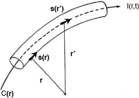
Figure 1: Geometry for thin-wire electric-field integral equation (from [7]).
Also, and the unprimed coordinates and denote the observation point location and the primed coordinates and the source location which accounts for the propagation time delay between the source and observation points. The differential operators in (5) are with respect to the observation coordinates. If we let and be the unit tangent vectors to at and then for a PEC wire the boundary condition is
| (6) |
with the applied field that causes the current and charge. When equation 6 is combined with equation 5, the following integral equation results:
| (7) |
where and is the wire radius at point and he charge is given by
| (8) |
Equation (7) provides the analytical basis for TWTD and is called an integral equation because the unknown quantities requiring solution are under the integral sign. The procedure used to develop a solution is called the moment method [6, 7]. Most of the numerical examples in the next section are obtained from TWTD, but for illustrative comparison some frequencydomain results obtained from the NEC (Numerical Electromagnetics Code) [8] are also included.
To conclude this introductory discussion it’s relevant to point out that there is a graphical approach to demonstrate the effects of charge acceleration known as the “E-Field Kink Method [8, 9] described next. This method is useful for developing a dynamic visualization of the radiation from a point charge as shown next in Section II. but is unlikely to be feasible for the current and charge sources on an extended object.
II. THE E-FIELD KINK MODEL OF RADIATION
Graphical displays of EM radiation fields can be developed without actually solving the MEs using what is known as the “E-field Kink Model of Radiation” [9, 10]. This is made possible by two properties of EM fields, (a) that a charge produces continuous electric-field lines of force and (b) that the speed of light has a finite value.
Consider a point charge located at the origin of a spherical coordinate system in an infinite, homogenous medium. The charge emanates or terminates a radially directed electric field whose lines of force are uniformly distributed in angle with a density proportional to the charge magnitude as in Fig. 2 (a). By convention these field lines originate on positive charge and terminate on negative charge or extend to infinity.
If the charge is instantaneously accelerated to velocity v and coasts for time its E -field lines will be as shown in Fig. 2 where a “kink” has developed in its field lines which has propagated a radial distance from the origin where c is the speed of light. Abruptly stopping the charge at time t1 causes another E-field kink to be produced that at time t2 later has now propagated a radial distance from the origin as illustrated in Fig. 2.
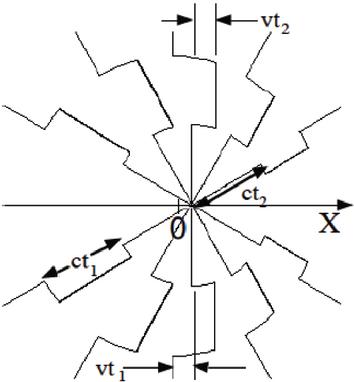
Figure 2: A snapshot of the E-field of a point charge that has been instantaneously accelerated to a speed v, abruptly stopped at time t1 and at an additional time interval t2 later (Fig. 1 from [15]).
Observe that following any of the field lines outward the two kinks are of opposite sign. This is a consequence of the acceleration term in equation (8) since the starting and stopping accelerations are of opposite sign. Note also in Fig. 2 that the length of the field kink gets longer in proportion to distance from the charge, associated with the fall off of the radiated E field and that there is no field kink, or radiation, in the direction of charge motion. Not shown in these plots is the accompanying H-field component with their vector cross product accounting for the Poynting vector power flow in equation (9).
A computer program, Radiation 2, was developed at Stanford University by Professor Blas Cabrerra and his students [11, 12] that develops a time sequence of plots to create a movie of the E-field lines for several kinds of chargeacceleration motion such as oscillatory, circular, etc. Two stills from this program are presented in Fig. 3. Included in the program are a choice of the geometrical motion and a selection of the peak charge speed and acceleration.
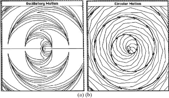
Figure 3: Single frames taken from an E-field kink computer program [12] for a point charge undergoing oscillatory linear motion (a) and moving at constant speed around a circle (b) (from [15]).
III. TIME-DOMAIN RESULTS USING TWTD
Electromagnetic radiation is obviously a time-domain phenomenon as it results from the acceleration of charge. Consequently it is most appropriate to examine the details of EM radiation from a time-domain perspective as is done below for a variety of problems. The well-validated computer model based on a time-domain electric-field integral equation for perfect electric conducting (PEC) wires called TWTD (thin wire time domain [5] was used to obtain the results that follow. Basically, these results can be characterized, as computer experiments that emulate what might be done using laboratory measurements were the appropriate equipment to be available. Further examples of the results that follow can be found in [9]. For time-domain modeling of antennas or scatterers, a Gaussian-shaped impulsive excitation is normally used. This produces time and space-limited current and charge pulses on the object whose impulsive far-fields can be associated with locations where they originate from the object being modeled. A Gaussian time-dependent excitation pulse used in TWTD is given by
| (9) |
where is a width parameter and determines the time at which the pulse maximum occurs. The simplest timedomain wire geometry is a straight wire, known as a dipole antenna when excited by a local voltage source. A dipole of length of 5.99 m is modeled with 599 segments of length m. A wire radius of and time step of are used throughout unless otherwise stated. The current and charge-density times light speed are shown at several time steps in Fig. 4 for excitation of the dipole antenna at segment 300 by a peak Gaussian pulse, an excitation used for all time-domain results presented in the following.
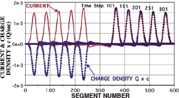
Figure 4: Charge density times light-speed and the current for a 599-segment wire excited at its center by a Gaussian voltage pulse at several time steps (Fig. 3.2 from [10]).
Several interesting observations can be made of the results of Fig. 4.
(a) The positive and _pulses_are numerically equal on the right-hand side of the dipole (i.e. ) but are of opposite signs on the left-half side. This is because a positive charge moving to the right produces a positive current, as also does a negative charge moving in the opposite direction to the left. Their numerical equality implies that the current and charge carry the same amount of energy, an effect that is discussed further in connection with Fig. 9.
(b) The amplitudes of the and pulses decay as they propagate outwards towards the ends of the wire dipole.
(c) The uniformly spaced pulses are apparently moving at a constant speed.
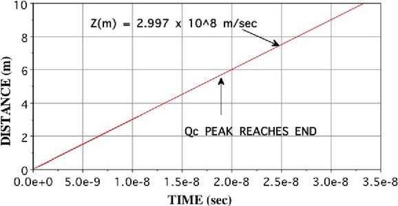
Figure 5: A time-distance plot for the data of Fig. 4 using additional time steps and a best-fit straight line.
The latter observation is confirmed in Fig. 5 where a best-fit straight line is shown on a time-distance plot for the 599 segment dipole based on the peaks of the rightward-propagating pulses some of which are included in Fig. 6. There is no apparent discontinuity effect upon to end reflection. The average speed of these pulses as determined from the best-fit line is , within of the input in TWTD. Time on this plot is measured from the pulse at 367 time steps on Fig. 4.
The electric far fields normal to dipole antennas of variable lengths as a function of time is plotted in Fig. 6 up to the time just beyond the time of the first end reflection of the outward propagating pulses. This plot reveals three different types of radiation. The first is due to the initial charge acceleration caused by the center-located voltage pulse. The second radiation pulses are due to the pulses reaching the wire ends and where they reflect and reverse direction. The source-caused radiation pulse is about half that of the segment wire, due to the fact that the source imparts a speed of to the outward-propagating pulses while end reflection involves a speed change of . The end-reflected peaks decrease with increasing dipole lengths due to an intermediate, or traveling-wave reflection effect that causes the decreasing magnitude of the reflected pulses.
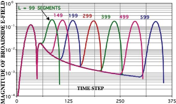
Figure 6: The magnitude of the relative broadside radiated electric fields in for various dipole lengths in 0.01 m long segments (Fig. 3.4 from [10]).
This reflection is continuous as the pulses propagate down the dipole arms due to the wave impedance of a constant-radius wire varying with distance from the feedpoint as shown by the admittance in Eq. (10) [13]. This would not occur if the arms of the dipole were cones instead, resulting in a length-independent wave impedance as shown in Eq. (11) [14]. The wave-impedance reflection is also responsible for the decreasing end radiation exhibited in Fig. 6.
| (10) | |
| (11) |
A plot of this propagation-caused radiated electric field is presented in Fig. 7 normalized to the amount of charge reflected per time step. The latter is obtained by integrating the amount of charge in the outgoing pulse at each time step to compute how much has been reflected. This plot is somewhat jagged since it involves the subtraction of two nearly equal numbers. Nevertheless, the match between the electric field and the reflected charge is on average within a few percent.
It’s interesting to compute the numerical ratio between and the corresponding radiated electric field for these 3 radiation mechanisms, defined here as an “Acceleration Factor” . This is demonstrated in Fig. 8 where the charge time variation multiplied by its AF is plotted with its associated radiated E-field. Although the values must be considered approximate as their computation is somewhat imprecise, the endreflected is estimated at 1.95 times that for the source , or about different from the value of 2 that might be expected. On the other hand the propagation is only 1.21 times that for the source. This might be inferred to be so much less than 2 because the reflection mechanism is “smoother” than reflecting from an open wire end.
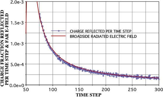
Figure 7: The time variation of the traveling-wave radiated electric field and the reflected charge steps (Fig. 13 from [16]).
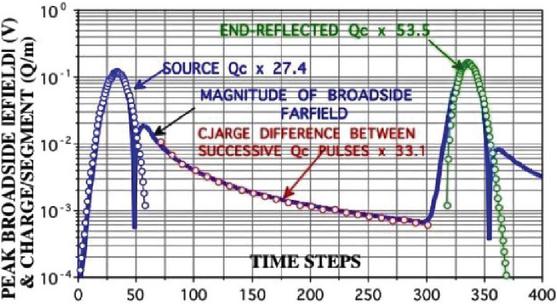
Figure 8: A combined plot of the propagation, source and end-reflected broadside E-field magnitudes and the respective time varying accelerated charges that produce them (Fig. 12 (b) from [10]).
The acceleration factors presented in Fig. 8 and using the equivalent approach for some other radiation mechanisms are summarized for reference in Table 1. While computing their values may be somewhat uncertain in an absolute sense, their ratios may be useful for comparing their relative influences in producing a radiated field.
Table 1: AF values for various radiation types
| Radiation Type | Acceleration Factor |
| Source: | 27.4 |
| Variable Wire Radius: | 29.2 |
| Right-Angle Bend: | 47.0 |
| Propagation: | 33.1 |
| Resistance Load: | 59.4 |
| End Reflection: | 53.5 |
A different way of demonstrating radiation effects for the 599-segment dipole is illustrated in Fig. 9. The current energy and charge energy measures integrated over the dipole as a function of time are obtained from
| (12) |
and
| (13) |
The energy computation in Eq. (13) treats the end segments of the dipole differently to account for the end current going to 0 on those segments.
The current, charge and total energy measures plotted as a function of time in Fig. 9. The initial energy buildup is dominated by the charge but after about 50 time steps the current and charge energies become equal, decaying smoothly together until the first end reflection. These effects are due to the source and propagation radiations. At each end reflection the current energy falls to 0 when all of the energy is due to the charge with a sharp decrease in the total energy. The opposite effect occurs when the end-reflected pulses meet at the center feedpoint with an almost imperceptible loss of the total energy.
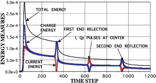
Figure 9: The current, charge and total energy measures as a function of time for an impulsively excited straight wire as a dipole antenna (Fig. 4.6 from [10]).
Differentiating the total energy of Fig. 9 with respect to time is useful to show the rate of the total energy loss as displayed in Fig. 10. These rate curves are rather noisy in appearance as this again involves the difference of nearly equal numbers, an effect that increases as the loss rate decreases by more than 2 orders of magnitude. It’s interesting to see that the loss rate is quite similar in each sequence. There is, however, between the first and second end reflections a slight “bump” of about 2 during the time interval when the charge pulses overlap as they pass through the center feedpoint.
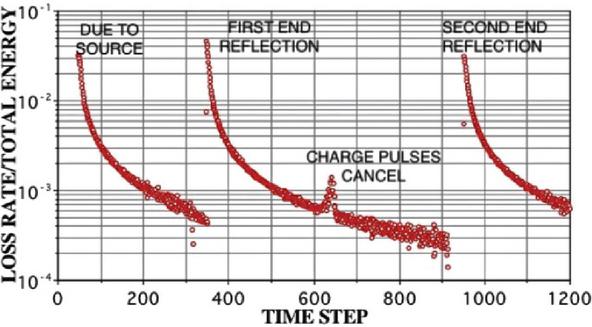
Figure 10: The differentiated total energy plot of Fig. 6 illustrating the doubling of the radiation-loss rate as the counter-propagating charge pulses meet at the center of the dipole (Fig. 4.8 from [10]).
This phenomenon occurs because the propagation of the counter-propagating-pulse radiation becomes coherent or additive over the far-field sphere. This effect is similar to what happens when 2 one-watt, frequency-domain point sources are brought together, the result of which is shown in Fig. 11. Their total radiated power increases in an oscillatory fashion as they are moved closer together until it doubles at zero separation.
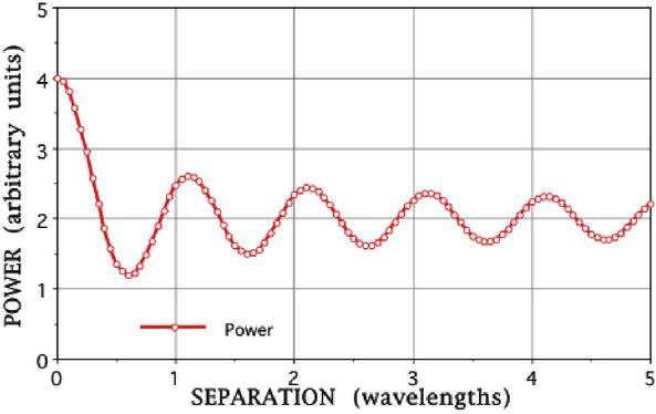
Figure 11: The power radiated by 2 unit-amplitude point sources as a function of their separation in wavelengths (Fig. 1 (b) from [17]).
The current, charge and total energy measures as a function of time for a 1.99 m straight wire excited by a normally incident impulsive plane wave is shown in Fig. 12. There is a periodic interchange between the charge and current energies as they each pass through successive oscillations of zero energy. The current (red) and charge (blue) distributions at 9 time samples to demonstrate this effect are exhibited in Fig. 13.
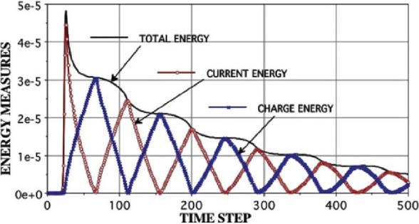
Figure 12: The current, charge and total energy measures as a function of time for an wire impulsively excited by a normally incident plane wave dipole (Fig. 4.18 from [10]).
The frequency-domain normalized Poynting vector along a 10-wavelength dipole obtained from is plotted in Fig. 14. It is somewhat analogous to the energy-measure time-domain result of Fig. 9 over the time of the exciting source turn on to the first end reflection. Differentiating this result yields the rate of radiated power-loss as a function of position in Fig. 15 for comparison with the energy-loss rate in the time domain of Fig. 10 [15]. Whereas the time-domain energy loss is monotonic except for the charge-pulse overlap, that for the frequency domain is lobed because the latter supports a standing-wave current.
A circular wire loop should be expected to exhibit a higher energy loss versus distance than a straight wire because the charge acceleration is greater than the dipole due to the loop’s curvature. This effect is illustrated in Fig. 17 where pulses are shown in the time domain at 100 time-step intervals on a dipole and loop 1,200 segments long. The loop peak is at time step 600 is incomplete because it is partially obscured by the counter-propagating pulse meeting it at the side opposite the feedpoint. The dipole is excited at segment 49 to avoid the first end reflection. Note that the loop pulses are moving slightly faster than those on the dipole because their associated electric fields straight-line path is shortened by the loop curvature.
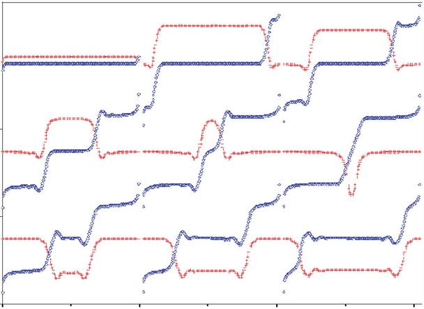
Figure 13: The current (red) and charge (blue) distributions at 9 time samples for an impulsive plane wave at normal incidence scattering from a straight wire reading left to right from the top dipole (Fig. 4.16 from [10]).
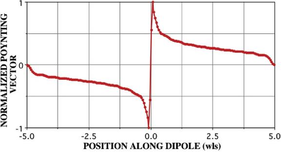
Figure 14: The on-surface Poynting vector obtained from NEC for a center-fed, 10-wavelength dipole with power flow to the left negative and to the right positive (Fig. 5 from [18]).
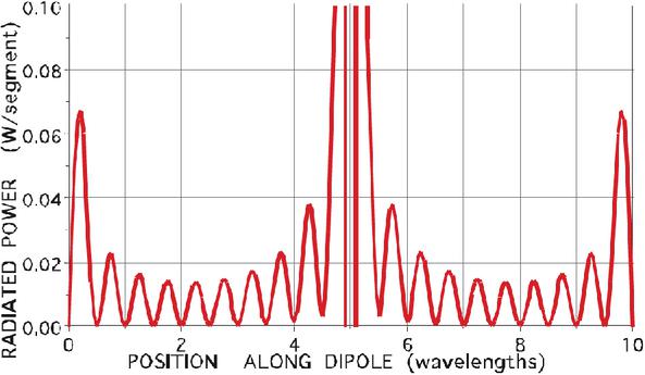
Figure 15: The differentiated Poynting-vector of Fig. 14 for a 10 -wavelength dipole (Fig. 6.8 (a) from [10]).
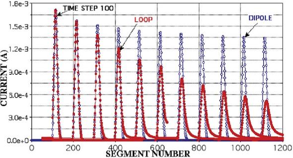
Figure 16: Comparison of the pulses on 1,200 segment dipoles and circular loops at 100-segment time steps (Fig. 3.5 (a) from [10]).
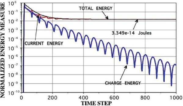
Figure 17: The current, charge, and total energies as a function of time step for a loop of 5 m ( 100 segment) circumference and wire radius of 0.02 m as a function the time step (Fig. 5.2 from [10]).
In a fashion similar to Fig. 9 for the dipole, the current, charge and total energies for the circular loop are presented in Fig. 17. There are two especially interesting features to be seen here as the current and total energies asymptotically approach constant values while the charge energy decreases towards zero in an oscillatory fashion. The oscillatory decay it exhibits occurs because each time the opposite-signed, oppositely propagating charge pulses meet moving around the loop, they cancel to produce alternating minima because their accelerations are radially inward and thus cancel. The charge energy eventually becomes zero as the loop radiates the time-dependent energy deposited by the impulsive excitation.
This results in a uniform, non-radiating, late-time current and charge neutrality around the loop. Interestingly, this current can be used to compute the inductance of the loop [16]. Actually, this is possible for literally any closed loop that can be modeled using TWTD or a similar computer model. Note the contrast with the late-time current and charge on an open object such as a dipole where both decay to zero as charge neutrality is restored.
IV. Conclusion
The results presented here demonstrate how EM radiation is caused by various kinds of impulsive charge acceleration for simple wire geometries using a time-domain computer model derived from the Maxwell Equations. The excitation, either a local voltage for an antenna or a distributed electric field for a scatterer, causes the initial acceleration. This excitation essentially begins the process and results in an effective speed increase of for the charge induced by the applied electric fields. Other various reflection mechanisms subsequently exhibit somewhat different acceleration effects and produce speed changes of , due to reversing the direction of the charge motion. These include propagation radiation because of the location-dependent wave impedance of a uniform-radius wire. Other reflection radiation is caused by open wire ends, changes in wire radius, sharp bends, smooth curves and impedance loads. These reflection accelerations are due to the electric fields that are terminated by charge on the wire and whose speed must match that of the fields in the medium
Appendix
The following information is provided for readers who might like to perform similar computer “experiments” using NEC or TWTD. The latest version of NEC, 4.2, continues to be distributed by Lawrence Livermore National Laboratory. Information concerning its availability and cost can be obtained at “https://softwarelicensing.llnl.gov/product/nec-v42”.
The TWTD code in a pdf Fortran file is available from the author via email at no cost, along with a user’s manual. Contact me at e.miller@ieee.org for any questions that you might have. Note that both codes include a feature called FARS (Far-field Analysis of Radiation Sources) [10] for determining the spatial distribution of radiated power from a PEC object. FARS was not included above because it wasn’t necessary to for this introductory presentation.
REFERENCES
1Assuming an object to be a PEC is a common boundary condition used in EM computer modeling and is acceptably accurate for most materials used for antennas and radar targets. This means that EM fields originate or terminate at the surface of an object on what are called equivalent sources. In particular, the normal electric field creates an excess of charge at its termination point depending on whether the E-field originates, causing positive charge or terminates, to cause negative charge at that point on the wire’s surface. The equivalent, essentially massless, charge density this creates follows the propagating EM field moving at light speed in the external medium. The validity of this model is confirmed by experimental measurements.
REFERENCES
[1] A. Liénard, “Champ électrique et magnétique produit par une charge électrique concentrée en un point et animée d’un movement quelconque,” L’éclairage Électrique, vol. 16, pp. 16–21, 1898.
[2] E. Wiechert, “Elektrodynamische elementargesetze,” Ann. Phys., vol. 4, pp. 667–689, 1901.
[3] K. Yee, “Numerical solution of initial boundary value problems involving Maxwell’s equations in isotropic media,” IEEE Transactions on Antennas and Propagation, vol. 14, no. 3, pp. 302–307, 1966.
[4] J. A. Landt, E. K. Miller, and M. L. Van Blaricum, WT-MBA.LL1B: A Computer Program for the Time-Domain Response of Thin-Wire Structures, Livermore, CA: Lawrence Livermore Laboratory, 1974.
[5] E. K. Miller, A. J. Poggio, and G. J. Burke, “An integro-differential equation technique for the time-domain analysis of thin-wire structures. Part I: The numerical method,” Journal of Computational Physics, vol. 12, pp. 24–48, 1973.
[6] R. F. Harrington, Field Computation by Moment Methods. New York, NY: Macmillan, 1968.
[7] E. K. Miller, “Computational electromagnetics,” in The Electrical Engineering Handbook, Richard C. Dorf, Ed. Boca Raton, FL: CRC Press, pp. 1028–1049, 1993.
[8] G. J. Burke, E. K. Miller, and A. J. Poggio, “The numerical electromagnetics code (NEC) – A brief history,” in 2004 IEEE Int. Antennas Propagat. Symp. Dig., vol. 42, pp. 2871–2874, June 2004.
[9] G. S. Smith, Classical Electromagnetic Radiation Cambridge: Cambridge University Press, 1997.
[10] E. K. Miller, Charge Acceleration and the Spatial Distribution of Radiation Emitted from Antennas and Scatterers. London: Institution of Engineering and Technology, 2023.
[11] B. Cabrera, Physics Simulations II: Electromagnetism, Academic Version. Santa Barbara, CA: Intellimation Library for the Macintosh, 1990.
[12] B. Cabrera and E. K. Miller, “Macintosh Movies for Teaching Undergraduate Electricity and Magnetism,” in 1986 International IEEE APS Symposium, Philadelphia, PA, 9–13 June 1986.
[13] J. Bach Anderson, “Admittance of infinite and finite cylindrical metallic antenna,” Radio Science, vol. 3, no. 6, pp. 607–621, 1968.
[14] C. A. Balanis, Antenna Theory: Analysis and Design. New York: Harper & Row Publishers, 1982.
[15] E. K. Miller and G. J. Burke, “A multi-perspective examination of the physics of electromagnetic radiation,” Applied Computational Electromagnetics Society (ACES) Journal, vol. 16, no. 3, pp. 190–201, 2001.
[16] E. K. Miller, “Comparison of the radiation properties of a sinusoidal current filament and a pec dipole of near zero radius,” IEEE Antennas and Propagation Society Magazine, vol. 48, no. 4, pp. 37–47, Aug. 2006.
[17] E. K. Miller, “Time-Domain Far-Field Analysis of Radiation Sources and Point-Source Coherence,” IEEE Antennas and Propagation Society Magazine, vol. 54, no. 2, pp. 100–108, Apr. 2012.
[18] E. K. Miller, “The differentiated on-surface Poynting vector as a measure of radiation loss from wires,” IEEE Antennas and Propagation Society Magazine, vol. 48, no. 6, pp. 21–32, Dec. 2006.
BIOGRAPHIES

Edmund K. Miller earned a B.S. (EE) in 1957 from Michigan Technological University (then known as Michigan College of Mining and Technology. His graduate work was done at the U. of Michigan, with an M.S. (Nuclear Engineering) in 1958, an M.S. (EE) in 1963 and a Ph.D. (EE) in 1965. His working career included 4 universities (Michigan Tech 1958–59, U. of Michigan 1959–68, Kansas U. 1985–1987 and Ohio U.1994–95); 3 companies (MBAssociates (1969–71, Rockwell International Science Center 1985–1987, and General Research Corporation (1987–1988); and 2 National Laboratories (Lawrence Livermore (1971–85 and Los Alamos (1989–1993). He has been actively retired since 1995 and has lived in Lincoln, CA since 2003.
His involvement in Computational Electromagnetics began in 1959 and continues to the present. He wrote a regular column “PCs for AP and Other EM Reflections” from 1985 to 2000 for the IEEE Antennas and Propagation Society. In addition to his nearly 200 journal articles and various society proceedings he edited the book “Time Domain Measurements in Electromagnetics” in 1986 and co-edited the IEEE reprint volume “Computational Electromagnetics: Frequency-Domain Moment Methods”. He wrote the 2023 book “Charge Acceleration and the Spatial Distribution of Radiation Emitted by Antennas and Scatterers” that summarized his work on radiation physics over the years, and another about to be published “Model-Based Parameter Estimation in Electromagnetics”.
Dr. Miller was the first president of ACES, of which he was a founding member, and is a Fellow of the IEEE and ACES.
ACES JOURNAL, Vol. 40, No. 11, 1055–1063
DOI: 10.13052/2025.ACES.J.401101
© 2025 River Publishers