Electromagnetic Shielding Effectiveness Prediction of Stacked, Chassis Based on Snow Ablation Optimizer Algorithm

Sen Wang¹, Hong Jiang¹, Xinbo Li¹, Xiaohui Wang², and Fengtao Xu²

¹College of Communication Engineering, Jilin University, Changchun, 130012, China, wangsen23@mails.jlu.edu.cn, jiangh@jlu.edu.cn, xb_li@jlu.edu.cn
²Research and Development Department, China Academy of Launch Vehicle Technology, Beijing, 100076, China, wang98421@163.com, sunshine-taotao@163.com

Submitted On: November 18, 2025; Accepted On: January 25, 2026

Abstract

Stacked chassis has wide application in aerospace integrated electronic systems. However, with irregular enclosure structure and multi-module integrated into small space, its electromagnetic shielding effectiveness (SE) prediction is a challenge problem. In this paper, a novel method of SE prediction for stacked chassis is proposed based on snow-ablation optimizer (SAO) algorithm. First, a dedicated model of stacked chassis is selected and the SE at five internal sampling points is obtained via full-wave numerical simulation. Then, building on the Robinson equivalent model combined with the generalized Baum-Liu-Tesche (BLT) equations, and exploiting the initial simulation data as priors, the characteristic parameters of the stacked chassis are achieved via the SAO algorithm. On this basis and under vertically polarized and normally incident plane wave, the SE is predicted at all the positions across the central axis normal to the incident face of the chassis. The prediction results enable identification of the optimal SE distribution along frequency axis inside the chassis, thereby informing the internal layout and placement of sensitive devices. The prediction curves agree well with the simulation results, which can overcome the large-error limitations of conventional analytical approaches for complex cavities.

Keywords: Electromagnetic shielding, Robinson equivalent model, shielding effectiveness prediction, snow-ablation optimizer, stacked chassis..

1 INTRODUCTION

Electromagnetic shielding is one of the most widely used techniques for protecting electronic equipment. The performance of a shielded enclosure is quantified by its shielding effectiveness (SE), which is the ratio of the electric field intensities at the locations of the monitoring point without and with the shielded case [1].

At present, there are three main methods to calculate the SE of the shielded cavities: experimental measurement, numerical simulation, and analytical algorithm. Measurements can better restore the real working scene of the shielding cavity and obtain more accurate measurement results. However, shielding rooms, microwave dark rooms, spectrum analyzers, and other experimental sites and expensive instruments are usually required. Hence, its cost is relatively high and, when the shielding cavity is located in a more complex environment, the experimental conditions are difficult to simulate and the limitations are greater.

Numerical calculation methods mainly include finite-difference time-domain (FDTD) algorithm [2, 3, 4, 5], method of moments (MoM) [6, 7, 8], transmission line matrix (TLM) algorithm [9, 10, 11], finite element method (FEM) [12] and some hybrid numerical algorithms [13, 14, 15, 16, 17, 18], which generally simulate the experimental scenarios through the simulation software, accurately build the complex model, and obtain the SE of the shielded cavity through the solution algorithm. However, to obtain accurate calculation results, the simulation process occupies a large amount of memory, takes long computation time, and requires high computer performance.

The analytical method occupies less memory with high computational efficiency, and is convenient for analyzing the effect of different parameter changes on the SE of the cavity. However, it is necessary to perform the equivalent processing of the shielding cavity during the modeling process. When the shielding cavity structure is relatively complex, the modeling process cannot be performed accurately, which is prone to cause deviations in the calculation results. A representative algorithm for the analytical calculation of SE of open rectangular cavities under plane wave irradiation is the cavity equivalent circuit model method proposed by Robinson et al. [19]. Many researchers have proposed improved analytical methods on this basis [20, 21, 22, 23, 24].

In recent years, driven by the demands of aerospace integrated electronic systems for “high integration, small form factor, and rapid deployment,” stacked-architecture chassis technology has rapidly progressed from proof-of-concept to engineering application. The stacked chassis consists of multiple functional modules stacked vertically and locked as a single assembly by four long through-bolts; internal board-to-board high-speed connectors mate directly to carry data and power. A typical unit is more compact than comparable VITA46 standardized VPX chassis and employs fully conduction-cooled thermal management. The structural features and operating environment of the stacked chassis are highly complex, making experimental measurements stringent and costly.

In this paper, to address the limitations of existing approaches, a novel method is presented for the SE prediction of a stacked-architecture chassis. First, a specific stacked chassis model is selected, and the SE at five internal sampling points is obtained via numerical simulation using the software of computer simulation technology (CST) [25]. Next, a mathematical model for SE calculation is formulated based on the Robinson equivalent model combined with the Baum-Liu-Tesche (BLT) equations. Using the initial simulation results as priors, the characteristic parameters of the stacked chassis are estimated through the snow-ablation optimizer (SAO) algorithm, thereby enabling SE prediction. The proposed method is low-cost and easy to implement compared with the experimental measurements; it avoids repeated modeling and substantially reduces computational resources relative to the numerical simulation approaches.

2 STACKED CHASSIS MODEL AND PROBLEM FORMULATION

2.1 Stacked-architecture chassis model

In this paper, a dedicated stacked-architecture chassis is selected as the research subject. Its model is shown in Fig. 1, and the chassis dimensions and connector cut-out locations are provided in Fig. 2. We can observe that, originating from a real engineering prototype, the chassis exhibits irregular distributions of apertures and seams as well as a complex internal structure, making conventional analytical approaches inadequate for accurately evaluating its SE. To address this, the apertures and seams are equivalently modeled using the Robinson equivalent-circuit method in conjunction with the BLT equations, and the characteristic parameters of the chassis equivalent circuit are estimated via the SAO algorithm. On this basis, the SE at all the positions along the central axis normal to the incidence face inside the chassis can be predicted.

Figure 1 Front and rear views of the stacked chassis model.

Figure 2 Dimensional schematic of the stacked chassis model.

2.2 SE calculation model based on Robinson equivalent model and BLT equations

The SE calculation for a simple shielded cavity using the Robinson equivalent model and BLT equations is first reviewed, after which it is refined for the stacked chassis characteristics and its characteristic parameters are optimized.

Based on the TLM theory, Robinson et al. proposed an equivalent transmission line model for a regular aperture-seam shielded cavity, and the SE of the shielded cavity can be calculated based on the equivalent model. Figure 3 shows a rectangular shielded cavity model, and Fig. 4 is its equivalent transmission line circuit of the shielded cavity. The dimensions of the shielded cavity are $a\times b\times d$, the thickness is $t$, and the dimensions of the rectangular aperture slit on the cavity surface are $l\times w$. Assume that the plane wave is incident vertically from the direction of the plane where the aperture slit is located, and the observation point $P$ is in the center axis of the plane wave incidence plane and is at a distance from the plane wave incidence plane.

Figure 3 A rectangular shielded cavity model.

Figure 4 Equivalent circuit of the shielded cavity based on transmission line equivalence method.

Equating the plane wave to a voltage source $V_0$ and an impedance $Z_0=377\mathrm{\Omega }$, the aperture in the shielded cavity is equivalent to the impedance, which is expressed as

$$Z_{ap}=\frac{1}{2}\frac{l}{a}j{Z}_{0s}\tan \frac{k_{0}l}{2},$$

(1)

where $k_0=2\pi /\lambda$, and

$$Z_{0s}=120{\pi }^2{\left[\ln \left(2\frac{1+\sqrt[4]{1-{(w_e/b)}^2}}{1-\sqrt[4]{1-{(w_e/b)}^2}}\right)\right]}^{-1},$$	(2)
$$w_e=w-\frac{5t}{4\pi }\left(1+\ln \frac{4\pi w}{t}\right).$$	(3)

Considering the shielded cavity as a waveguide, if only the $T{E}_{10}$ mode is propagated, the characteristic impedance of the shielded cavity and the propagation constant are respectively shown as

$$Z_g=Z_0/\sqrt{1-{(\lambda /2a)}^2},$$	(4)
$$k_g=k_0\sqrt{1-{(\lambda /2a)}^2}.$$	(5)

Based on this, we can effectively compute the SE of an ideal enclosure with a central slot.

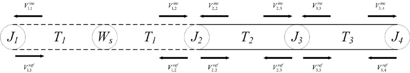
Figure 5 The corresponding signal-flow graph.

According to the circuit model in Fig. 4, the corresponding signal-flow graph is drawn as Fig. 5. Here, node $J_1$ denotes the external observation point of the enclosure, $J_2$ denotes the aperture, $J_3$ denotes the internal observation point, and $J_4$ denotes the rear end of the enclosure. $W_s$ represents the source in the equivalent circuit. Tube 1 corresponds to free-space wave propagation outside the enclosure, while Tubes 2 and 3 represent wave propagation inside the enclosure. $V^{inc}$ indicates the incident wave at a node, and $V^{ref}$ indicates the reflected wave.

Let ${\mathbf{S}}_1$ and ${\mathbf{S}}_2$ represent the scattering matrices at nodes $J_2$ and $J_3$, respectively, written as

$${\mathbf{S}}_1=\left[\begin{array}{cc}\frac{Y_0-Y_g-Y_{ap}}{Y_0+Y_g+Y_{ap}}\hfill & \frac{2Y_g}{Y_0+Y_g+Y_{ap}}\hfill \\ \frac{2Y_0}{Y_0+Y_g+Y_{ap}}\hfill & \frac{Y_g-Y_0-Y_{ap}}{Y_0+Y_g+Y_{ap}}\hfill \end{array}\right],$$	(8)
$${\mathbf{S}}_2=\left[\begin{array}{cc}0\hfill & 1\hfill \\ 1\hfill & 0\hfill \end{array}\right],$$	(11)

where $Y_0,Y_g,Y_{ap}$ denote the admittances of the free space, transmission line, and aperture, respectively.

Based on the propagation characteristics of waves in free space and inside the waveguide, the system propagation relation equations is derived as

$\left[\begin{array}{c}{V}_{1,1}^{ref}\\ V_{1,2}^{ref}\\ V_{2,2}^{ref}\\ V_{2,3}^{ref}\\ V_{3,3}^{ref}\\ V_{3,4}^{ref}\end{array}\right]=$	$\left[\begin{array}{cccccc}0& e^{{\gamma }_0{l}_0}& 0& 0& 0& 0\\ e^{{\gamma }_0{l}_0}& 0& 0& 0& 0& 0\\ 0& 0& 0& e^{{\gamma }_0{d}_i}& 0& 0\\ 0& 0& e^{{\gamma }_0{d}_i}& 0& 0& 0\\ 0& 0& 0& 0& 0& e^{{\gamma }_0(d-d_i)}\\ 0& 0& 0& 0& e^{{\gamma }_0(d-d_i)}& 0\end{array}\right]$	(24)
	$\times \left[\begin{array}{c}{V}_{1,1}^{inc}\\ V_{1,2}^{inc}\\ V_{2,2}^{inc}\\ V_{2,3}^{inc}\\ V_{3,3}^{inc}\\ V_{3,4}^{inc}\end{array}\right]-\left[\begin{array}{c}{V}_0\\ 0\\ 0\\ 0\\ 0\\ 0\end{array}\right]$	(37)

where $l_0$ is the distance from the incident wave to the enclosure, and ${\gamma }_0=j{k}_0$ denotes the free-space propagation constant. The $6\times 6$ square matrix in (37) is the propagation matrix. Let ${\gamma }_g$ denote the waveguide propagation constant, i.e.,

$${\gamma }_g=j{k}_g=j{k}_0\sqrt{1-{(\lambda /2a)}^2},$$

(38)

and define the node reflection coefficient $\rho$ as

$$\rho \stackrel{\mathrm{\Delta }}{=}\frac{V^{ref}}{V^{inc}},$$	(39)
$$\rho =\frac{Z_L-Z_C}{Z_L+Z_C},$$	(40)

where $Z_L$ is the load impedance and $Z_C$ is the characteristic impedance. From the relationships between the incident and reflected waves at each node, the scattering-relation equations can be obtained as

$$\left[\begin{array}{c}{V}_{1,1}^{ref}\\ V_{1,2}^{ref}\\ V_{2,2}^{ref}\\ V_{2,3}^{ref}\\ V_{3,3}^{ref}\\ V_{3,4}^{ref}\end{array}\right]=\left[\begin{array}{cccccc}{\rho }_1& 0& 0& 0& 0& 0\\ 0& S_{11}^1& S_{12}^1& 0& 0& 0\\ 0& S_{21}^1& S_{22}^1& 0& 0& 0\\ 0& 0& 0& S_{11}^2& S_{12}^2& 0\\ 0& 0& 0& S_{21}^2& S_{22}^2& 0\\ 0& 0& 0& 0& 0& {\rho }_4\end{array}\right]\left[\begin{array}{c}{V}_{1,1}^{inc}\\ V_{1,2}^{inc}\\ V_{2,2}^{inc}\\ V_{2,3}^{inc}\\ V_{3,3}^{inc}\\ V_{3,4}^{inc}\end{array}\right],$$

(41)

where ${\rho }_1$ denotes the reflection coefficient at node 1, ${\rho }_1=0$. ${\rho }_4$ is the reflection coefficient at node 4, ${\rho }_4=-1$. The $6\times 6$ matrix in (41) composes a total scattering matrix $\mathbf{S}$.

$\left[\begin{array}{c}{V}_{1,1}\\ V_{1,2}\\ V_{2,2}\\ V_{2,3}\\ V_{3,3}\\ V_{3,4}\end{array}\right]=$	$\left[\begin{array}{cccccc}1+{\rho }_1& 0& 0& 0& 0& 0\\ 0& 1+S_{11}^1& S_{12}^1& 0& 0& 0\\ 0& S_{21}^1& 1+S_{22}^1& 0& 0& 0\\ 0& 0& 0& 1+S_{11}^2& S_{12}^2& 0\\ 0& 0& 0& S_{21}^2& 1+S_{22}^2& 0\\ 0& 0& 0& 0& 0& 1+{\rho }_4\end{array}\right]$	(42)
	$\times {\left[\begin{array}{cccccc}-{\rho }_1& e^{{\gamma }_0{l}_0}& 0& 0& 0& 0\\ e^{{\gamma }_0{l}_0}& -S_{11}^1& -S_{12}^1& 0& 0& 0\\ 0& -S_{21}^1& -S_{22}^1& e^{{\gamma }_0{d}_i}& 0& 0\\ 0& 0& e^{{\gamma }_0{d}_i}& -S_{11}^2& -S_{12}^2& 0\\ 0& 0& 0& -S_{21}^2& -S_{22}^2& e^{{\gamma }_0(d-d_i)}\\ 0& 0& 0& 0& e^{{\gamma }_0(d-d_i)}& -{\rho }_4\end{array}\right]}^{-1}\left[\begin{array}{c}0.5V_0{e}^{{\gamma }_0(l_0/2)}\\ -0.5V_0{e}^{{\gamma }_0(l_0/2)}\\ 0\\ 0\\ 0\\ 0\end{array}\right]$

The synthesized voltage at nodes $V(x)$ is defined as (42), where $V_{3,3}$ is the voltage at the internal observation point $P$, denoted as $V_p$, and the voltage at the observation point when the enclosure is absent is represented as $V_p^{{}^{\prime }}$. Here ${\mathbf{S}}_1$ and ${\mathbf{S}}_2$ are respectively denoted as

$${\mathbf{S}}_1=\left[\begin{array}{cc}{S}_{11}^1& S_{12}^1\\ S_{21}^1& S_{22}^1\end{array}\right],$$	(45)
$${\mathbf{S}}_1=\left[\begin{array}{cc}{S}_{11}^2& S_{12}^2\\ S_{21}^2& S_{22}^2\end{array}\right].$$	(48)

Then the SE at the observation point can be calculated by

$$SE=-20\log (V_p/V_p^{{}^{\prime }}).$$

(49)

2.3 Problem formulation

The cavity model in the previous section is assumed to be an ideal shielding body with a single aperture seam, which is a rectangular body with a regular shape except for the structure of the aperture seam. However, the surface of the stacked-architecture chassis to be studied has small irregular aperture seams. Its structure is complicated, the transmission line equivalent model obtained by the above-mentioned method has low accuracy, and the results of the shielding SE have a large deviation. So it is necessary to improve the equivalent model to enhance its accuracy.

According to the equivalent transmission-line model, the equivalent impedances of the aperture/slot and of the shielded cavity are the primary factors governing model accuracy. Therefore, (1), (2), (4), and (5) are modified so that they capture the characteristics of a stacked-architecture chassis. Let $k_1$ denote the aperture-location parameter of the stacked chassis; $k_2$ and $k_3$ the aperture-shape parameters, and $k_4$ an enclosure structural parameter. By incorporating $k_1$, $k_2$, $k_3$, $k_4$ into (1), (2), (4), and (5), the accuracy of the stacked-chassis equivalent model can be improved.

The resulting SE calculation model for the stacked-architecture chassis is shown in (50),

$$\{\begin{array}{cc}\hfill Z_{ap}& =\frac{1}{2}\frac{k_1{k}_2}{a}j{Z}_{0s}\tan \frac{k_0{k}_2}{2}\hfill \\ \hfill Z_{0s}& =120{\pi }^2{\left[\ln \left(2\frac{1+\sqrt[4]{1-{\left(k_3/b\right)}^2}}{1-\sqrt[4]{1-{\left(k_3/b\right)}^2}}\right)\right]}^{-1}\hfill \\ \hfill Z_g& =Z_0/\left(k_4\sqrt{1-{\left(\lambda /2a\right)}^2}\right)\hfill \\ \hfill k_g& =k_0{k}_4\sqrt{1-{\left(\lambda /2a\right)}^2}\hfill \\ \hfill \left[\begin{array}{c}{V}_{1,1}\\ V_{1,2}\\ V_{2,2}\\ V_{2,3}\\ V_{3,3}\\ V_{3,4}\end{array}\right]& =\left[\begin{array}{cccccc}1+{\rho }_1& 0& 0& 0& 0& 0\\ 0& 1+S_{11}^1& S_{12}^1& 0& 0& 0\\ 0& S_{21}^1& 1+S_{22}^1& 0& 0& 0\\ 0& 0& 0& 1+S_{11}^2& S_{12}^2& 0\\ 0& 0& 0& S_{21}^2& 1+S_{22}^2& 0\\ 0& 0& 0& 0& 0& 1+{\rho }_4\end{array}\right]\hfill \\ & \times {\left[\begin{array}{cccccc}-{\rho }_1& e^{j{k}_0{d}_0}& 0& 0& 0& 0\\ e^{j{k}_0{d}_0}& -S_{11}^1& -S_{12}^1& 0& 0& 0\\ 0& -S_{21}^1& -S_{22}^1& e^{j{k}_g{d}_1}& 0& 0\\ 0& 0& e^{j{k}_g{d}_1}& -S_{11}^2& -S_{12}^2& 0\\ 0& 0& 0& -S_{21}^2& -S_{22}^2& e^{j{k}_g{d}_2}\\ 0& 0& 0& 0& e^{j{k}_g{d}_2}& -{\rho }_4\end{array}\right]}^{-1}\left[\begin{array}{c}0.5V_0{e}^{{\gamma }_0(l_0/2)}\\ -0.5V_0{e}^{{\gamma }_0(l_0/2)}\\ 0\\ 0\\ 0\\ 0\end{array}\right]\hfill \\ \hfill SE& =-20{\log }_{10}\left(V_0/V_{3,3}\right)\hfill \end{array}$$

(50)

where $V_0$ is the equivalent voltage source of the incident wave; $k_0=2\pi /\lambda$ is the free-space propagation constant; $Z_0$ is the intrinsic impedance of free space; $\lambda =c/f$ is the incident wavelength; $f$ is the incident frequency; $c$ is the speed of light; $a$ is the height of chassis; and $b$ is the length of the chassis bottom edge on the plane-wave incident face, where

$$\{\begin{array}{c}{S}_{11}^1=\left(\frac{1}{Z_0}-\frac{1}{Z_g}-\frac{1}{Z_{ap}}\right)/\left(\frac{1}{Z_0}+\frac{1}{Z_g}+\frac{1}{Z_{ap}}\right)\hfill \\ S_{12}^1=\left(2\times \frac{1}{Z_g}\right)/\left(\frac{1}{Z_0}+\frac{1}{Z_g}+\frac{1}{Z_{ap}}\right)\hfill \\ S_{21}^1=\left(2\times \frac{1}{Z_0}\right)/\left(\frac{1}{Z_0}+\frac{1}{Z_g}+\frac{1}{Z_{ap}}\right)\hfill \\ S_{22}^1=\left(\frac{1}{Z_g}-\frac{1}{Z_0}-\frac{1}{Z_{ap}}\right)/\left(\frac{1}{Z_0}+\frac{1}{Z_g}+\frac{1}{Z_{ap}}\right),\hfill \end{array}$$

(55)

$$\{\begin{array}{c}{S}_{11}^2=S_{22}^2=0\\ S_{21}^2=S_{21}^2=1.\end{array}$$

(58)

Since the stacked chassis consists of multiple structurally similar and relatively enclosed modules, this work predicts SE using a single module as a representative case. The enclosure’s characteristic parameters are identified from SE data at five interior sampling points within the module. The procedure is as follows.

[(1)]

(1) Sample the simulated SE at five sampling points located along the central axis of the incident face of the stacked-chassis module. Denote the resulting data by the matrix $\mathbf{S}$; these samples specify the target locations for identifying the enclosure characteristic parameters of the selected module.

(2) Determine the enclosure’s characteristic parameters using the above SE prediction model for the stacked chassis, and compute the theoretical SE of the selected module. Denote the computed results as the matrix ${\mathbf{S}}^{\prime }$, which serves as the predicted SE for the selected module enclosure.

(3) Formulate an objective function to drive the position-parameter vector toward the target. The objective function is given by

$$\min P={|\mathbf{S}(n)-{\mathbf{S}}^{\prime }(n,i)|}^2,$$

(59)

where $\mathbf{S}(n)$ denotes the sampled value of the SE at the $n$-th frequency point, and ${\mathbf{S}}^{\prime }(n,i)$ denotes the theoretically computed SE for the $i$-th individual in the population at the $n$-th frequency point.

(4) The fitness evaluation function is defined as

$$F(n,i)\stackrel{\mathrm{\Delta }}{=}\frac{1}{\tau +P(n,i)},$$

(60)

where $\tau =0.001$. A larger $F(n,i)$ (corresponding to a smaller $P(n,i)$) indicates stronger fitness, whereas a smaller $F(n,i)$ (corresponding to a larger $P(n,i)$) indicates weaker fitness.

3 ALGORITHM TO SOLVE SHIELDING EFFECTIVENESS PREDICTION PROBLEM

3.1 Basic CST simulation settings

A Gaussian electromagnetic pulse from the CST electromagnetic simulation software is used as the simulated signal source. The pulse has a higher electric field intensity and allows frequency-domain coverage and field intensity of the waveform to be customized through the operating frequency, thereby simulating more severe and complex electromagnetic environment. The approximate expression of the Gaussian electromagnetic pulse is

$f(t)$	$={\displaystyle \frac{\kappa A}{\pi (t-c)}}\sin \left({\displaystyle \frac{(B_H-B_L)(t-c)}{2}}\right)$
	$\times e^{j\frac{(B_H+B_L)(t-c)}{2}},$	(61)

where $A=20$ V/m is the peak value of the electric field strength, $\kappa$ is the correction factor, $B_H$ and $B_L$ are the maximum and minimum frequencies, and $c$ is the time shift amount. The time-domain and frequency-domain waveforms of the Gaussian electromagnetic pulse are shown in Fig. 6.

The SE at internal monitoring points of the chassis under vertically polarized and vertically incident plane waves is simulated using CST electromagnetic software, where the electric field intensity at these points before and after adding the chassis is obtained and used to calculate the SE. The simulation frequency range is set from 0 to 18 GHz, and the chassis material is set to PEC. The simulation diagram is shown in Fig. 7.

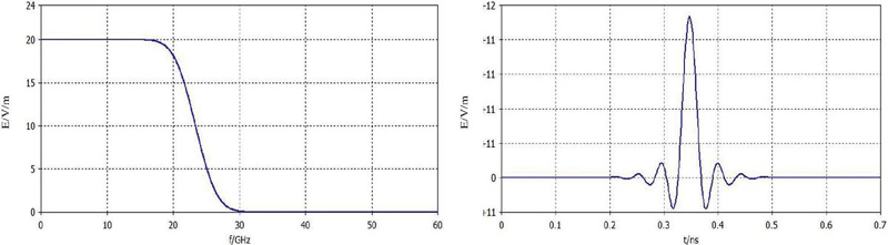
Figure 6 The frequency-domain and time-domain waveforms of the Gaussian electromagnetic pulse.

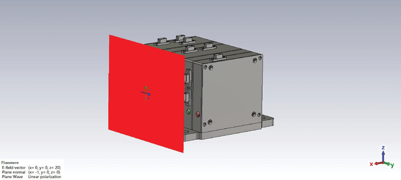
Figure 7 The simulation diagram using CST.

3.2 Snow ablation optimizer algorithm for SE, prediction

Over the past two decades, metaheuristic algorithms (MAs) have been widely employed across numerous fields to solve a broad range of complex engineering problems. In particular, when tackling nonconvex, highly nonlinear, nonsmooth, and even dynamic real-world problems, MAs exhibit greater general applicability than traditional mathematical optimization methods owing to their gradient-free nature and structural simplicity [26, 27].

The snow ablation optimizer [28, 29] aims to balance global exploration and local exploitation in the solution space, improving convergence efficiency while preserving population diversity, thereby addressing the shortcomings of existing methods on complex problems. It can mitigate premature convergence compared with traditional algorithms such as particle swarm optimization (PSO).

Inspired by snow ablation, SAO maps physical phase-change behaviors to search strategies: sublimation corresponds to dispersed global exploration, melting corresponds to local exploitation around elite solutions, and evaporation represents an adaptive adjustment between these two modes. During optimization, the algorithm dynamically coordinates diffusive exploration and focused exploitation.

(1) Population, In the SAO optimization process, the population consists of $N$ candidate solutions maintained in parallel and is represented by the position matrix

$${\mathbf{Z}}^{(t)}={[z_{i,j}^{(t)}]}_{N\times Dim}={[{\mathbf{z}}_1^{{(t)}^T},\mathrm{\cdots },{\mathbf{z}}_N^{{(t)}^T}]}^T,$$

(62)

where ${\mathbf{z}}_i^{(t)}=[z_{i,1}^{(t)},z_{i,2}^{(t)},\mathrm{\cdots },z_{i,Dim}^{(t)}]$ denotes the parameter vector of the $i$-th individual at iteration $t$, and $Dim$ is the dimension of the decision variables. In this paper, $Dim=4$ for four parameters. The initial population is generated uniformly at random within the lower and upper bounds $\mathbf{L}$ and $\mathbf{U}$:

$${\mathbf{Z}}^{(0)}=\mathbf{L}+\mathbf{R}\odot (\mathbf{U}-\mathbf{L}),$$

(63)

where $\mathbf{R}\in {[0,1]}_{N\times Dim}$ and $\odot$ denotes the element-wise (Hadamard) product. To balance global exploration and local exploitation, SAO dynamically partitions the population index set into an exploration subpopulation and an exploitation subpopulation.

Meanwhile, the population centroid is computed to characterize the overall distribution and assist the position update:

$${\overline{\mathbf{z}}}^{(t)}=\frac{1}{N}\sum _{i=1}^N{\mathbf{z}}_i^{(t)}.$$

(64)

This design enables the algorithm to rapidly locate promising regions in the early stage while maintaining diversity in later iterations to mitigate premature convergence.

(2) Fitness function, At the $n$-th discrete frequency point, the CST post-processed SE at the $m$-th sampling location ($m=1,\mathrm{\cdots },5$) is denoted by ${\mathbf{S}}_m(n)$. For the $i$-th individual (candidate parameter vector) ${\mathbf{z}}_i$ in the population, the SE predicted by the Robinson-equivalent model and BLT equations is ${\mathbf{S}}_m^{\prime }(n,i)$. The objective function is defined as the sum of squared errors over the five sampling locations:

$$P(n,i)=\sum _{m=1}^5{({\mathbf{S}}_m(n)-{\mathbf{S}}_m^{\prime }(n,i))}^2.$$

(65)

Since SAO is implemented as a fitness-maximization scheme (larger fitness is better), the fitness function is constructed by mapping the objective value as

$$F(n,i)=\frac{1}{\epsilon +P(n,i)},$$

(66)

where $\epsilon =0.001$ is introduced to avoid division by zero when $P(n,i)\to 0$ and to improve numerical stability. Therefore, a larger $F(n,i)$ (i.e., a smaller $P(n,i)$) indicates better agreement between the model prediction and the CST results at the five sampling points. In each iteration, SAO evaluates $F(n,i)$ for all individuals and selects the one with the maximum fitness as the current best solution for subsequent updates and elitist guidance.

(3) Sublimation, melting, and evaporation Sublimation (exploration phase): The sublimation phase corresponds to the physical process in which snow (or meltwater derived from snow) transforms into vapor. The resulting irregular particle motion leads to a highly dispersed search behavior; therefore, SAO models it as global exploration using Brownian motion. For standard Brownian motion, the step length is drawn from a standard normal distribution with probability density function

$$f_{BM}(x;0,1)=\frac{1}{\sqrt{2\pi }}{e}^{-\frac{x^2}{2}}.$$

(67)

Accordingly, the position-update equation for each individual in the exploration phase is given by (3.2),

$\mathbf{z}_{n,i}^{}{}_{}{}^{(t+1)}$	$=Elit{e}_n(t)+B{M}_{n,i}(t)\odot (R_1\cdot ({\mathbf{g}}_n(t)-\mathbf{z}_{n,i}^{}{}_{}{}^{(t)})$
	$+(1-R_1)\cdot (\overline{\mathbf{z}}_n^{}{}_{}{}^{(t)}-\mathbf{z}_{n,i}^{}{}_{}{}^{(t)}))$	(68)

where $\mathbf{z}_{n,i}^{}{}_{}{}^{(t)}$ denotes the position (candidate parameter vector) of the $i$-th individual at iteration $t$ for the $n$-th frequency point; $B{M}_{n,i}(t)$ is the Brownian-motion random step vector, $B{M}_{n,t}(t)\sim \mathbb{N}(0,1)$; $R_1\in [0,1]$ is a random factor that weights two guidance directions; ${\mathbf{g}}_n(t)$ is the current global-best individual at the $n$-th frequency point; $Elit{e}_n(t)$ denotes an individual randomly selected from the elite pool at the $n$-th frequency point (the elite pool consists of the best, second-best, and third-best individuals); $\overline{\mathbf{z}}_n^{}{}_{}{}^{(t)}$ is the population centroid for the $n$-th frequency point. As shown in (3.2), the sublimation operator enables dispersed exploration via Brownian diffusion while incorporating elitist and population-level guidance, thereby improving global search capability and alleviating premature convergence.

Melting (exploitation phase): The melting phase corresponds to the heating-induced transition from snow to liquid water, and it is mapped in SAO to local exploitation around the current best solutions. In this phase, search agents are encouraged to perform denser, fine-grained searches in the neighborhood of the current global best, while information exchange with the population centroid helps accelerate convergence toward high-quality regions and reduces stagnation in a single basin of attraction. To model the progressively strengthened exploitation pressure over iterations, the classical degree-day snowmelt model is adopted. Its general form is

$$M=DDF\times (T-T_1),$$

(69)

where $M$ denotes the snowmelt rate, $T$ is the daily mean air temperature, and $T_1$ is the base (threshold) temperature, typically set to $0^{\circ }C$. By setting $T_1=0$, (69) becomes

$$M=DDF\times T,$$

(70)

where $DDF$ denotes the degree-day factor. To introduce a time-varying exploitation schedule, the $DDF$ is updated as

$$DD{F}_n(t)=0.35+0.25\times \frac{e^{\frac{t}{ite{r}_{\max }}-1}}{e-1},$$

(71)

where $ite{r}_{\max }$ is the maximum number of iterations, and $t$ is the current iteration. Defining

$$T(t)=e^{-\frac{t}{ite{r}_{\max }}},$$

(72)

the snowmelt rate at the $n$-th frequency point is written as

$$M_n(t)=DD{F}_n(t)\times T(t).$$

(73)

Subsequently, within the melting operator, the position-update equation for each individual is given by (74),

$\mathbf{z}_{n,i}^{}{}_{}{}^{(t+1)}$	$=M_n(t)\cdot {\mathbf{g}}_n(t)+B{M}_{n,i}(t)$	(74)
	$\odot (R_1\cdot ({\mathbf{g}}_n(t)-\mathbf{z}_{n,i}^{}{}_{}{}^{(t)})$
	$+(1-R_1)\cdot (\overline{\mathbf{z}}_n^{}{}_{}{}^{(t)}-\mathbf{z}_{n,i}^{}{}_{}{}^{(t)}))$

where $R_2$ is a random number in $[-1,1]$ used to enhance information exchange among individuals. As indicated in (74), the melting operator strengthens exploitation through the time-varying factor $M_n(t)$ while maintaining necessary activity via mild stochastic perturbations, thereby enabling efficient refinement around promising regions.

Evaporation (dynamic adjustment): The evaporation phase corresponds to the physical process in which meltwater further evaporates into vapor. Algorithmically, SAO maps this process to a dynamic adjustment of the exploration–exploitation balance: as iterations proceed, the algorithm gradually increases the tendency toward irregular, highly dispersed motion (vapor-like diffusion), which helps maintain population diversity, suppress overly aggressive convergence, and strengthen global search capability.

To implement this mechanism, a dual-subpopulation scheme is used in the SAO. At iteration $t$ for the $n$-th frequency point optimization, the whole population $P$ is randomly partitioned into an exploration subpopulation $P_a^{(t)}$ (sublimation) and an exploitation subpopulation $P_b^{(t)}$ (melting):

$$\begin{array}{c}P=P_a^{(t)}\cup P_b^{(t)},P_a^{(t)}\cap P_b^{(t)}=\mathrm{\varnothing },\\ |P_a^{(t)}|=N_a(t),|P_b^{(t)}|=N_b(t),N_a(t)+N_b(t)=N.\end{array}$$

(75)

Initially, the two subpopulations are of equal size:

$$N_a(1)=N_b(1)=\frac{N}{2}.$$

(76)

Then, a linear schedule is applied to gradually enlarge exploration while reduce exploitation (consistent with the MATLAB implementation):

$N_a(t+1)$	$=\min (N,N_a(t)+1),$	(77)
$N_b(t+1)$	$=N-N_a(t+1).$	(78)

Accordingly, the exploration and exploitation ratios are

$${\rho }_a(t)=\frac{N_a(t)}{N},{\rho }_b(t)=\frac{N_b(t)}{N}=1-{\rho }_a(t),$$

(79)

where ${\rho }_a(t)$ increases with $t$. Under this “evaporation–diffusion” metaphor, the algorithm realizes a temporal scheduling of the exploration–exploitation ratio and promotes coordination between global and local search throughout the run.

(4) Complete position-update, The complete position-update equation of the SAO is given by (80). The entire population is effectively represented as a position matrix. Accordingly, in the foregoing equation, $inde{x}_a$ and $inde{x}_b$ denote the index sets of individuals belonging to $P_a$ and $P_b$, respectively, within this matrix.

$$\{\begin{array}{cc}& Elit{e}_n(t)+B{M}_{n,i}(t)\odot (R_1\cdot ({\mathbf{g}}_n(t)-\mathbf{z}_{n,i}^{}{}_{}{}^{(t)})\hfill \\ & +(1-R_1)\cdot (\overline{\mathbf{z}}_n^{}{}_{}{}^{(t)}-\mathbf{z}_{n,i}^{}{}_{}{}^{(t)})),i\in index{}_a\hfill \\ & M_n(t)\cdot {\mathbf{g}}_n(t)+B{M}_{n,i}(t)\odot (R_1\cdot ({\mathbf{g}}_n(t)-\mathbf{z}_{n,i}^{}{}_{}{}^{(t)})\hfill \\ & +(1-R_1)\cdot (\overline{\mathbf{z}}_n^{}{}_{}{}^{(t)}-\mathbf{z}_{n,i}^{}{}_{}{}^{(t)})),i\in index{}_b\hfill \end{array}$$

(80)

In the SAO algorithm, after updating the positions, the fitness values of all individuals associated with each frequency point are evaluated. If the maximum fitness in the current generation exceeds the pre-update maximum, the original position parameters of the corresponding individual are replaced with its current position parameters; otherwise, the original individual is retained. The procedure then proceeds to the next iteration, and the update operation is repeated cyclically.

4 GLOBAL ALGORITHM DESIGN

Based on the above problem model established in this paper and the introduction of the solution algorithm, the global algorithm design is carried out for the problem model. The flowchart of the SAO algorithm for SE prediction is shown in Fig. 8.

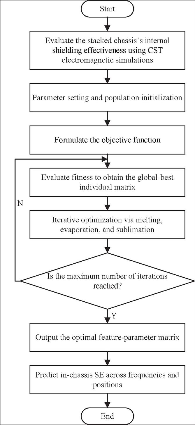
Figure 8 Overall algorithm flowchart.

The main steps of the algorithm are as follows:

Step 1, evaluation the SE of five sampling points using CST. Since the stacked-architecture chassis comprises multiple similar, relatively enclosed modules, we take the module enclosure shown in Fig. 9 as a representative example. Along the central axis normal to the plane-wave incident face inside this module, five reference points, labeled A, B, C, D, and E, are selected. The excitation is a short-duration pulsed plane wave with a peak electric-field strength of 20 V/m; the frequency range is set from 10 kHz to 18 GHz, and the polarization is vertical. Using the simulation, we obtain the SE curves at the five sampling points inside the module enclosure. The locations of A–E are shown in Fig. 9. These curves are then discretely sampled and arranged into a matrix $\mathbf{S}$, which serves as the target data for identifying the characteristic parameters of the module enclosure. The sampled curves are shown in Fig. 10.

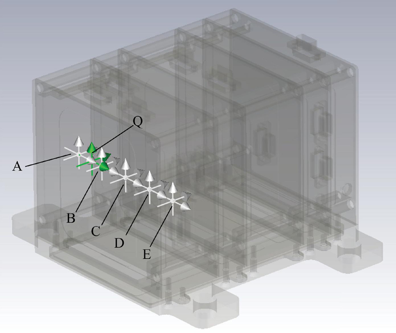
Figure 9 Locations of the five sampling points (A–E).

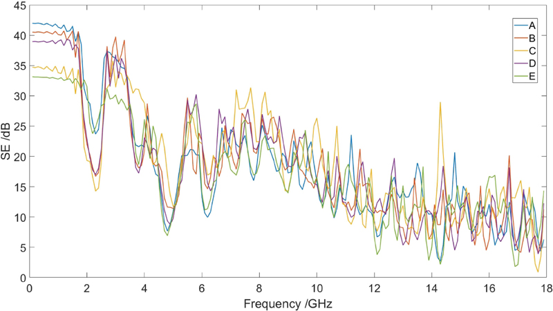
Figure 10 Shielding-effectiveness sampling curves at the selected sampling points inside the module enclosure.

Step 2, SAO parameter settings and population initialization. The decision-variable dimension and physical constraints are first determined, and lower/upper bounds are specified accordingly. Meanwhile, the target matrix $\mathbf{S}$ obtained in Step 1 is indexed by the unified discrete frequency list to form frequency-wise target data for subsequent per-frequency optimization. SAO control parameters are then specified (e.g., population size $N=100$ and number of maximum iteration $ite{r}_{\max }=200$ in this work). The population is randomly initialized within the prescribed bounds to ensure feasibility and adequate coverage: each individual carries four decision variables corresponding to the chassis characteristic parameters in the equivalent model, and the Brownian random vector is generated from a standard normal distribution. After initialization, fitness values are evaluated once and an elite pool (e.g., best/second-best/third-best individuals) is formed to support elitist guidance in subsequent updates. The population representation, initialization, and the definitions of centroid follow the preceding SAO description.

Step 3, equivalent-model evaluation, fitness construction, and fitness assessment. For each discrete frequency point, the candidate parameter vector of an individual is used to evaluate the equivalent model: based on the Robinson equivalent-circuit representation combined with the BLT equations, the model-predicted SE at the five sampling points is obtained at that frequency. Using the objective and fitness definitions in (65) and (66), the mismatch between the predicted SE and the target SE values (the corresponding column of $\mathbf{S}$) is computed to yield the fitness of each individual. At the end of each iteration, the current best and historical best solutions are updated, and the elite pool and required population statistics (e.g., centroid) are refreshed to provide best/elite/centroid guidance for the next update.

Step 4, update each individual’s position via the three SAO operators: sublimation, melting, and evaporation. At each iteration, the evaporation mechanism dynamically partitions the population into an exploration subpopulation and an exploitation subpopulation, and different update operators are applied accordingly. To ensure physical feasibility, boundary-constraint handling is applied to the individual parameters after each position update, followed by the next round of fitness evaluation and elitist retention.

Step 5, the algorithm halts when the SAO reaches the preset maximum number of iterations. The best individual in the population attains the highest fitness and exhibits the closest agreement with the simulated SE results. Across all frequency points, the position parameters of the optimal individuals are assembled into a feature-parameter matrix comprising four groups of features, denoted $k_{n1},k_{n2},k_{n3},k_{n4}$, where $n$ indexes the $n$-th frequency point. Here, $k_{n1}$ represents the aperture-location parameters of the stacked chassis, $k_{n2}$ and $k_{n3}$ represent the aperture-shape parameters, and $k_{n4}$ represents the chassis structural parameters. This set can be expressed by an $n_{\max }\times 4$ matrix $\mathbf{Z}\mathrm{\_}best$, denoted as

$$\mathbf{Z}\mathrm{\_}best=\left[\begin{array}{cccc}\begin{array}{c}{k}_{1,1}\\ k_{2,1}\\ \mathrm{⋮}\\ k_{n_{\max },1}\end{array}& \begin{array}{c}{k}_{1,2}\\ k_{2,2}\\ \mathrm{⋮}\\ k_{n_{\max },2}\end{array}& \begin{array}{c}{k}_{1,3}\\ k_{2,3}\\ \mathrm{⋮}\\ k_{n_{\max },3}\end{array}& \begin{array}{c}{k}_{1,4}\\ k_{2,4}\\ \mathrm{⋮}\\ k_{n_{\max },4}\end{array}\end{array}\right],$$

(81)

where $n_{\max }$ denotes the total number of selected frequency points. Using the global optimum identified by the SAO, namely, the optimal individual matrix $Z_{best}$, we can compute the SE at the $Q$ designated points within the selected module enclosure.

Step 6: Using the extracted feature-parameter matrix, analytically compute the SE at the predesignated $Q$ locations inside the selected module enclosure, and the resulting analytical SE values are validated by comparison with the CST simulation results at the same $Q$ locations.

Step 7: Based on the extracted feature-parameter matrix, the SE distribution at multiple interior locations of the selected module is predicted across different frequency points. Regions exhibiting superior electromagnetic shielding at each frequency are identified, thereby providing guidance for internal cable routing and for the placement of sensitive components/modules within the chassis.

5 ALGORITHM PERFORMANCE ANALYSIS

5.1 Analysis of sample size and computational resource usage

First, the two frequency-domain electric-field intensity curves at each sampling location—measured with and without the chassis protection—are post-processed in CST to obtain the corresponding SE spectrum at the sampling locations. The resulting SE frequency-domain data are then exported in ASCII format for external processing. In MATLAB, the exported SE spectrum contains a total of 1859 frequency samples. The data are subsequently resampled onto a uniform frequency grid, ranging from 0.1 GHz to 18 GHz with a step size of 0.1 GHz, yielding 180 frequency-domain samples used for the SAO iterations. At each discrete frequency point, the SAO optimizer takes the simulated SE values at the five sampling locations as the target outputs and performs the parameter update accordingly. Therefore, five data values are used per frequency point, and the optimization is carried out sequentially over all frequency points, resulting in a total of 900 frequency-domain scalar samples used in the overall procedure.

Table 1 Comparison of runtime and peak memory usage between the full-wave CST simulation and the proposed SAO-assisted analytical method

Method	Runtime	Peak Memory
Full-wave CST simulation	110 min 33 s	1413 MB
Proposed method	73.38 s	4444.48 MB

The overall computational cost is primarily determined by the number of fitness evaluations, and is approximately proportional to the product of the number of frequency points, population size, maximum number of iterations, and number of sampling points. When a denser frequency grid is adopted during sampling, the SAO algorithm must perform a larger number of independent per-frequency iterative optimizations; however, this also yields a denser discrete sequence of “frequency–enclosure characteristic parameters,” enabling the subsequent frequency-domain SE prediction to better match the simulation results and thereby reducing errors introduced by frequency discretization and interpolation.

Compared with performing a full-wave numerical simulation of the chassis directly in CST, the proposed approach shifts the computational burden from “full-wave broadband solving of a complex 3D structure” to “a single full-wave simulation to obtain SE spectra at a small number of sampling points + parameter identification based on an equivalent model + fast analytical prediction.” Specifically, the CST full-wave simulation uses the time-domain solver Hexahedral TLM, which discretizes the computational domain into a hexahedral mesh equivalently represented by a transmission-line network and updates the electromagnetic fields in the time domain through iterative node scattering and link propagation to obtain a broadband response. However, such time-domain grid-based methods typically require a sufficiently fine mesh and long time stepping to satisfy accuracy and energy-decay termination criteria, resulting in a high computational time cost. As summarized in Table 1, under the same hardware conditions, a single CST simulation for obtaining the SE spectrum at the probe locations takes approximately 110 min 33 s with a peak memory usage of about 1413 MB. In contrast, our MATLAB implementation performs uniform-frequency resampling of the exported SE spectrum, and applies SAO-based iterative identification at each frequency point using the SE values at five sampling locations as target outputs; the complete work-flow of “parameter extraction + SE prediction” takes approximately 73.38 s with a peak memory usage of about 4444.48 MB. Therefore, relative to a single full-wave CST simulation, the proposed approach can reduce the runtime by roughly one order of magnitude, at the expense of increased memory consumption due to population-based iterations and data-structure storage. More importantly, when SE must be evaluated repeatedly for multiple interior locations and layout schemes, the cost of full-wave CST simulations scales approximately linearly with the number of cases, whereas the proposed method requires only a small amount of full-wave data as priors and can rapidly generate broadband, multi-location SE predictions, thereby significantly reducing the overall computational cost for iterative engineering design.

5.2 Analysis of prediction results

Based on the extracted feature-parameter matrix, the SE at the $Q$-point within the selected module enclosure is predicted and compared with the CST simulation results at the same location to verify predictive accuracy. The $Q$-point location is shown previously in Fig. 9. A comparison between the predicted and simulated SE at the $Q$-point is presented in Fig. 11. The two SE curves exhibit a high degree of agreement, sharing the same overall trend with limited discrepancies, thereby demonstrating the accuracy and validity of the predictions.

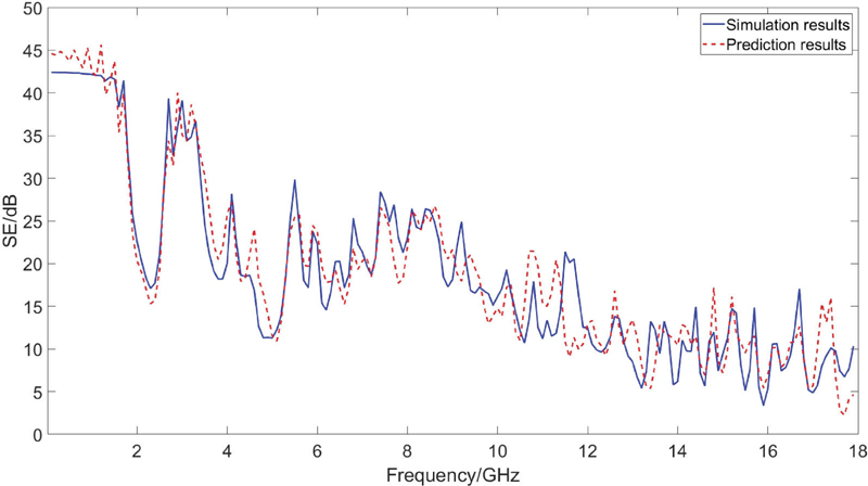
Figure 11 Comparison of the predicted and the simulated shielding effectiveness at $Q$-point location.

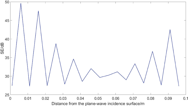
Figure 12 Effect of distance from plane wave incident surface on shielding effectiveness at 4 GHz frequency point.

Based on the extracted feature-parameter matrix, the SE at other interior locations of the selected module enclosure is predicted across different frequency points. Locations exhibiting relative advantages and disadvantages in SE at each frequency are analyzed to provide guidance for internal routing and for the placement of sensitive components.

As shown in Fig. 12, at 4 GHz the dependence of SE on the distance from the plane-wave incidence surface is presented. The results indicate that, at 4 GHz, the SE inside the selected module enclosure is generally between 25 dB and 35 dB; at distances of 0.006 m, 0.016 m, 0.081 m, and 0.091 m from the incidence surface, the enclosure exhibits comparatively higher SE. The maximum SE of 49 dB occurs at a distance of 0.006 m. Accordingly, sensitive components may be preferentially placed within 0–0.03 m from the plane-wave incidence surface.

As shown in Fig. 13, at 16 GHz the dependence of SE on the distance from the plane-wave incidence surface is presented. The results indicate that, at 16 GHz, the SE inside the selected module enclosure is generally between 5 dB and 20 dB; at distances of 0.016 m and 0.056 m from the incidence surface, the enclosure exhibits comparatively higher SE. The maximum SE of 29 dB occurs at 0.016 m. Accordingly, sensitive components may be preferentially placed near 0.016 m and 0.056 m from the plane-wave incidence surface.

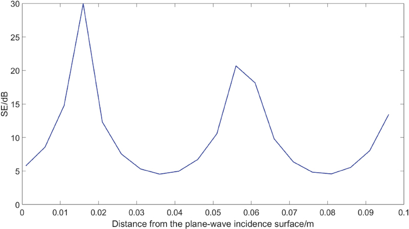
Figure 13 Effect of distance from plane wave incident surface on shielding effectiveness at 16 GHz frequency point.

Taking 9 GHz frequency point as an example, the fitness value at each iteration is obtained to compare the SAO with the conventional PSO algorithm, thereby evaluating the convergence behavior of the SAO. The resulting convergence curves are shown in Fig. 14. As can be seen from Fig. 14, our SAO-based algorithm converges significantly faster than the PSO: the SAO reaches the global optimum at the 19th iteration, whereas the PSO does not find the optimum until the 86th iteration. These results indicate that the SAO exhibits clearly superior convergence performance compared with the commonly used PSO algorithm.

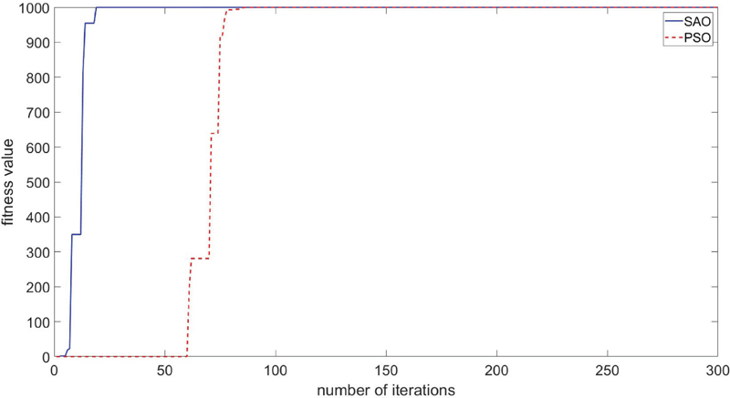
Figure 14 Convergence performance comparison of SAO and PSO algorithms.

6 CONCLUSION

We investigated the prediction of SE for the stacked chassis in this paper. An optimization problem model for the stacked chassis is formulated and the SAO-based solver is developed. The proposed approach balances exploration and exploitation, mitigates premature convergence, and better avoids local optima in complex search spaces, thereby improving equivalent-modeling prediction accuracy while substantially reducing computational cost. It can predict the SE of stacked chassis in complex environment, and yield SE prediction curves at multiple interior locations across frequencies. These results provide guidance for internal wiring and the placement of sensitive components.

References

[1] J. E. Bridges, “Proposed recommended practices for the measurement of shielding effectiveness of high-performance shielding enclosures,” IEEE Transactions on Electromagnetic Compatibility, vol. EMC-10, pp. 82–94, 1968.

[2] B. Jinjun, Z. Gang, and W. Lixin, “EMC simulation based on FDTD analysis considering uncertain inputs with arbitrary probability density,” IEEE Transactions on Electromagnetic Compatibility, vol. 34, pp. 82–94, 2019.

[3] A. Taflove, “Review of the formulation and applications of the finite-difference time-domain method for numerical modeling of electromagnetic wave interactions with arbitrary structures,” Wave Motion, vol. 10, pp. 547–582, 1988.

[4] N. V. Kantartzis, “Multi-frequency higher-order Adi-FDTD solvers for signal integrity predictions and interference modeling in general EMC applications,” Wave Motion, vol. 25, pp. 1046–1060, 2010.

[5] L. Avazpour, S. W. Belling, M. L. King, S. Schmidt, and I. Knezevic, “Field–potential finite-difference time-domain (FiPo FDTD) technique for computational electromagnetics,” Journal of Computational Electronics, vol. 24, p. 119, 2025.

[6] J. Bai, G. Zhang, L. Wang, and T. Wang, “Uncertainty analysis in EMC simulation based on improved method of moments,” Applied Computational Electromagnetics Society (ACES) Journal, vol. 31, pp. 66–71, 2016.

[7] D. Omri, M. Aidi, and T. Aguili, “A comparison of three temporal basis functions for the time-domain method of moments (TD-MoM),” Journal of Computational Electronics, vol. 19, pp. 750–758, 2020.

[8] J. Bai, B. Hu, H. Cao, and J. Zhou, “Uncertainty analysis method for EMC simulation based on the complex number method of moments,” Progress in Electromagnetics Research Letters, vol. 121, pp. 7–12, 2024.

[9] W. J. R. Hoefer, “The transmission-line matrix method-theory and applications,” IEEE Transactions on Microwave Theory and Techniques, vol. 33, pp. 7–12, 1985.

[10] P. Russer and J. A. Russer, “Application of the transmission line matrix (TLM) method to EMC problems,” in 2012 Asia-Pacific Symposium on Electromagnetic Compatibility, pp. 141–144, 2012.

[11] N. S. Dončov, B. Milovanovic, and Z. Stanković, “Extension of compact TLM airvent model on rectangular and hexagonal apertures,” Applied Computational Electromagnetics Society (ACES) Journal, vol. 26, pp. 64–72, 2011.

[12] Z. Kubik and J. Skala, “Shielding effectiveness simulation of small perforated shielding enclosures using FEM,” Energies, vol. 9, p. 129, 2016.

[13] F. Chao and S. Zhongxiang, “A hybrid FD-MoM technique for predicting shielding effectiveness of metallic enclosures with apertures,” IEEE Transactions on Electromagnetic Compatibility, vol. 47, pp. 456–462, 2005.

[14] M. Ranasinghe and V. Dinavahi, “Massively parallel hybrid TLM-PEEC solver and model order reduction for 3D nonlinear electromagnetic transient analysis,” IEEE Transactions on Electromagnetic Compatibility, vol. 67, pp. 667–678, 2025.

[15] X. Q. Zheng, Z. Y. Huang, Y. Q. Liang, and H. Y. Duan, “Rapid calculation method of ultrathin dielectric layer shielding efficiency based on CNTD-FDTD method,” in 2024 IEEE International Conference on Computational Electromagnetics (ICCEM), pp. 1–3, Apr. 2024.

[16] R. Qi, Y. Ding, Y. Du, H. Cai, L. Jia, and X. Xiao, “Hybrid TDPEEC/FDTD method for lightning transient analysis in solar panels,” IEEJ Transactions on Electrical Electronic Engineering, vol. 17, p. 1, 2022.

[17] X. He, M. Chen, and B. Wei, “A hybrid algorithm of 3-D explicit unconditionally stable FDTD and traditional FDTD methods,” IEEE Antennas and Wireless Propagation Letters, vol. 23, pp. 1–5, 2024.

[18] A. A. Lodhi, Y. Zhu, and O. Gassab, “Improved hybrid FDTD method for complex thin wire structures inside enclosure for accurate differential-mode prediction,” IEEE Transactions on Electromagnetic Compatibility, vol. 67, pp. 1–13, 2025.

[19] M. P. Robinson, “Analytical formulation for the shielding effectiveness of enclosures with apertures,” IEEE Transactions on Electromagnetic Compatibility, vol. 40, pp. 240–248, 1998.

[20] A. Rabat, P. Bonnet, K. E. K. Drissi, and S. Girard, “Analytical formulation for shielding effectiveness of a lossy enclosure containing apertures,” IEEE Transactions on Electromagnetic Compatibility, vol. 60, pp. 1384–1392, 2018.

[21] A. A. Ivanov, A. V. Demakov, M. E. Komnatnov, and T. R. Gazizov, “Semi-analytical approach for calculating shielding effectiveness of an enclosure with a filled aperture,” Electrica, vol. 22, 2022.

[22] A. A. Ivanov, M. E. Komnatnov, and T. R. Gazizov, “Analytical model for evaluating shielding effectiveness of an enclosure populated with conducting plates,” IEEE Transactions on Electromagnetic Compatibility, vol. 62, pp. 2307–2310, 2020.

[23] A. Rabat, P. Bonnet, K. E. K. Drissi, and S. Girard, “An analytical evaluation of the shielding effectiveness of enclosures containing complex apertures,” IEEE Access, vol. 9, pp. 147191–147200, 2021.

[24] J.-C. Zhou and X.-T. Wang, “An efficient method for predicting the shielding effectiveness of an apertured enclosure with an interior enclosure based on electromagnetic topology,” Applied Computational Electromagnetics Society (ACES) Journal, vol. 37, pp. 1014–1020, 2022.

[25] CST Studio Suite [Online]. Available: http://www.cst.com

[26] Q. Li, S.-Y. Liu, and X.-S. Yang, “Influence of initialization on the performance of metaheuristic optimizers,” Applied Soft Computing, vol. 91, p. 106193, 2020.

[27] H. Su, D. Zhao, A. A. Heidari, L. Liu, X. Zhang, M. Mafarja, and H. Chen, “RIME: A physics-based optimization,” Neurocomputing, vol. 532, pp. 183–214, 2023.

[28] L. Deng and S. Liu, “Snow ablation optimizer: A novel metaheuristic technique for numerical optimization and engineering design,” Expert Systems With Applications, vol. 225, p. 120069, 2023.

[29] W. Chen, Z. Wang, Y. Yang, S. Wang, H. Wang, and Y. Ayaz, “Research on path planning of mobile robots based on snow ablation optimizer,” in 2024 43rd Chinese Control Conference (CCC), Kunming, China, pp. 4351–4356, 2024.

Biographies

Sen Wang received the B.S. degree in Electronic Information Engineering from Tianjin University of Technology, Tianjin, China, in 2023. He is currently pursuing the M.S. degree in New-Generation Electronic Information Technology with Jilin University, Changchun, China. His current research interests include simulation analysis of electromagnetic environmental effects, electromagnetic compatibility, and electromagnetic protection for electronic equipment.

Hong Jiang (corresponding author) received the B.S. degree in Radio Technology from Tianjin University, Tianjin, China, in 1989, the M.S. degree in Communication and Electronic System from Jilin University of Technology, Changchun, China, in 1996, and the Ph.D. degree in Communication and Information System from Jilin University, Changchun, China, in 2005. From 2010 to 2011, she worked as a visiting research fellow at McMaster University, Canada. Currently, she is a professor at the College of Communication Engineering, Jilin University, China. Her research fields focus on electromagnetic compatibility and signal processing for radar and wireless communications.

Xinbo Li received the B.S. degree in Automation from Jilin University, Changchun, China, in 2002 and the M.S. and Ph.D. degrees in Control Theory and Control Engineering from Jilin University, Changchun, China, in 2005 and 2009, respectively. Currently, he is a professor at the College of Communication Engineering, Jilin University, China. His research interests focus on electromagnetic protection, electromagnetic environment perception, intelligent signal recognition and processing.

Xiaohui Wang received the M.S. degree in China. He is currently a researcher in Research and Development Center, China Academy of Launch Vehicle Technology, Beijing, China. He is engaged in long-term research on advanced integrated electronic optimization design.

Fengtao Xu received the M.S. degree in mechanics from Xi’an Jiaotong University, China. He is currently a senior engineer at the Research and Development Center, China Academy of Launch Vehicle Technology, Beijing, China. He is primarily engaged in integrated design-related fields such as overall design of electromechanical systems, electrical design, and electromagnetic design.

ACES JOURNAL, Vol. 41, No. 01, 81–94
DOI: 10.13052/2026.ACES.J.410109
© 2026 River Publishers