A Novel Multibranch-Linear-Linear Basis Function Based Adaptive Accuracy Enhanced Method for MFIE and CFIE From Multiscale PEC Targets
Yu Wang1*, Jie Cheng1, 2, Yu Zhang1, Lei Yu1, Liu-Yang Shen1, and Sheng Liu1
1Key Laboratory of Advanced Science and Technology on High Power Microwave Northwest Institute of Nuclear Technology, Xi’an 710049, China
wangyuxidian@foxmail.com, zhangyu@nint.ac.cn, 1047272896@qq.com,
shenliuyang@nint.ac.cn, liusheng@nint.ac.cn
2Key Laboratory for Physical Electronics and Devices of the Ministry of Education School of Electronic Science and Engineering, Faculty of Electronic and Information Engineering,
Xi’an Jiaotong University, Xi’an 710049, China
jaecheng@163.com
*Corresponding author
Submitted On: December 24, 2025
Accepted On: February 22, 2026
ABSTRACT
In this paper, we propose a novel Multibranch-Linear-Linear basis function based adaptive accuracy enhanced (MB-LLB-AAE) method to solve the scattering problem from multiscale perfect electric conductor (PEC) targets. The calculation accuracy of traditional magnetic-field integral equation (MFIE) and combined field integral equation (CFIE) is not as good as that of electric-field integral equation (EFIE) under the same mesh size. The proposal of MBLL basis function has solved the accuracy problem of MFIE and CFIE when calculating multiscale PEC targets to a certain extent. However, a MB-LL basis function has two unknowns on a common edge, thus generating a prohibitive computational cost when calculating multiscale targets. Based on this problem, we propose the novel MB-LLB-AAE method, which not only effectively reduces the consumption when calculating multiscale targets, but also maintains an accuracy similar to that of using the MB-LL basis function only. Several numerical examples prove the advantages of the proposed method.
Keywords: Adaptive accuracy enhanced (AAE) method, combined-field integral equation (CFIE), magnetic-field integral equation (MFIE), multibranch RWG basis function (MB-LL), multiscale objects..
1 INTRODUCTION
With the rapid development of high-power microwaves, the simulation of scattering properties of targets becomes more and more important [1, 2, 3]. The surface integral equation (SIE) method has gradually become a more common method for calculating scattering problems because of its advantages in computing consumption [4, 5, 6]. The most widely used equations in SIE are the electric-field integral equation (EFIE) [7], the magnetic-field integral equation (MFIE) [8] and the combined-field integral equation (CFIE) [9]. However, MFIE and CFIE are not as accurate as EFIE when using the same size mesh [10, 11, 12]. The main reasons for this problem are two aspects [13]. One is that, although the integral kernel can be calculated accurately in MFIE, the integral kernel has the singularity of high order points [14]. Second, one of the MFIE is a regular integral. When the source triangles and the test triangles are close enough and the integral points are selected on the edges and vertices, a solid angle error will occur in the process of singularity extraction [15]. In order to solve this problem, many solutions are proposed [16, 17, 18, 19]. Among these methods, two are relatively representative. One of them uses the Linear-Linear (LL) basis function to improve calculation accuracy [20]. The LL basis function has a higher order than the RWG basis function, thus achieving higher calculation accuracy. However, the unknown quantity on a common edge of the LL basis function is 2. Therefore, if only the LL basis function is used for calculation, it will bring an excessive number of unknowns. Another method is the accuracy enhanced-CFIE (AE-CFIE) method which improves the computational accuracy of CFIE by mixing CFIE with EFIE. Although this method improves the accuracy of CFIE to a certain extent, it sacrifices convergence and does not consider a multiscale scenario at the same time [21].
The calculation of multiscale targets is also a key issue that needs to be considered. It is difficult to guarantee the accuracy of the calculation if the large mesh is used to mesh the whole target, and a large amount of unknown quantity will be produced if the fine mesh is used. For solving the multiscale problems, a series of methods were proposed [22, 23, 24, 25].
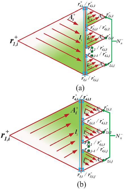
Figure 1 Schematic diagram of the two kinds of MB-LL basis function.
Recently, a multibranch-RWG (MB-RWG) basis function was proposed to solve the problem of multiscale target computation [26]. The MB-RWG basis function replaces the negative triangle of the RWG basis function to several branches, and guarantees the continuity of the current. By defining the MB-RWG basis function at the junction of the regions divided by different size mesh, the calculation of multiscale targets can be realized effectively, and it is relatively easy to achieve [27]. In [28], we proposed the construction method of multibranch LL basis function (MB-LL), which solved the accuracy problems of MFIE and CFIE when calculating multiscale targets. However, in [28], we only considered using the MB-LL basis function for calculation, which brings a large number of unknowns.
To address both multiscale problems and the issue that the full-domain application of MB-LL basis functions would double the number of unknowns, we extend the AE-CFIE method appropriately. We employ LL and MB-LL basis functions in regions that have a significant impact on computational accuracy, while using RWG and MB-RWG basis functions in other regions. In this manner, the number of unknowns associated with a single common edge is 2 only in the LL-based regions, whereas it is 1 in the RWG-based regions, thus effectively reducing the total number of unknowns. Based on this idea, in this paper we propose a novel multibranch-Linear-Linear basis function based adaptive accuracy enhanced (MB-LLB-AAE) method. The core innovations of this paper are summarized into three aspects.
• We applied MB-RWG to the AE-CFIE method. Since AE-CFIE is essentially a hybrid of EFIE and CFIE (replacing eligible components with EFIE), the introduction of EFIE degrades the convergence to a certain extent. To tackle this problem, we introduced MB-LL basis functions to further optimize the equation, thus developing the MB-LLB-AAE method. To the best of our knowledge, this is the first attempt to implement the MB scheme in the AE-CFIE framework.
• The proposed method is the first to introduce LL basis functions into the AE-CFIE framework and, combined with the MB scheme, it forms a novel approach more suitable for the calculation of multiscale targets.
• We propose a brand-new replacement strategy for MB-LL basis functions, which is different from the conventional AE-CFIE method. Specifically, for eligible common edges, their corresponding triangle pairs are determined, and all basis functions contained in these triangle pairs are replaced with MB-LL basis functions.
We use several numerical examples to prove the superiority of the proposed method in calculating the scattering problem from multiscale targets.
2 DEFINITION OF THE MB-LL AND THE CONSTRUCTION METHOD OF THE IMPEDANCE MATRIX
Schematic diagrams of the two kinds of MB-LL basis functions are shown in Fig. 1. The two kinds of LL basis functions can be expressed as [28]:
| (1e) | |
| (1j) |
where indicates that the expression belongs to the -th MB-LL basis function, indicates the expression belong to the -th negative branch of the MB-LL basis function, superscript is intended to demonstrate the expression belongs to positive triangle/negative branch, is the area of the triangle, is the domain of the integration, is the length of the common side, , and represent the three vertices of the positive triangle, while and represent the three vertices of the negative branch. The specific positions of the vertices are shown in Fig. 1. represents the normal vector of a triangle or branch. It should be noted that the current distribution over an MB-LL basis function is non-uniform. The distribution of current intensity is illustrated in Fig. 1, where a darker color indicates a stronger current. In addition, the degrees of freedom (DoF) of an MB-LL basis function are twice those of an MB-RWG basis function. Therefore, the global application of LL and MB-LL basis functions will significantly increase the number of unknowns. For perfect electric conductor (PEC) targets, EFIE and MFIE are defined as:
| (4) |
where is the distance from the field point to the source point, and are the position vectors of the field point and the source point, is the free space wave number, is the free space wave impedance, is the incident wave electric field, and is the surface current. is expanded by the RWG basis functions and MBRWG basis functions. By linear combination of the EFIE and MFIE in a certain proportion (: ), CFIE can be constructed as:
| (5) |
Here, if only LL basis functions and MB-LL basis functions are adopted in the computation, the current density needs to be expanded as:
| (6) |
Substituting (6) into (2) and then applying the Galerkin testing method yields the matrix equation, which can be explicitly written as:
| (11) | ||
| (14) |
It should be noted that the matrix forms of , and in (31) can be found in [28] and will not be elaborated here. It should be emphasized that (6) and (31) correspond to the case where only LL basis functions and MB-LL basis functions are used for computation. In this paper, current density is expanded by employing RWG, MB-RWG, LL, and MB-LL basis functions simultaneously. Accordingly, (6) is extended as:
| (15) |
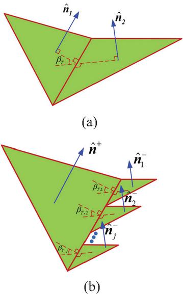
Figure 2 Schematic diagram of the dihedral angle (a) when using traditional conformal mesh and (b) when using nonconformal mesh.
Similarly, (31) is extended as:
| (20) | ||
| (29) |
Herein, the approach for handling singularities is adopted from [29]. It should be noted that the MB method requires some “special” treatment for meshes of different sizes; that is, the endpoints of the positive shared edges in one basis function must be aligned with those of the negative shared edges. If only the LL-basis functions and MB-LL basis functions are used to expand the current density , the number of unknowns obtained will be twice that when using the RWG basis functions and MB-RWG basis functions. This is unacceptable for the analysis of large-scale targets.
3 CONSTRUCTION RULES OF THE ADAPTIVE ACCURACY ENHANCED METHOD
To construct the AAE method, we referred to [21]. First, we need to define a dihedral angle . For traditional conformal triangles, we identify the positive and negative triangles corresponding to each common side. Next, we determine the specific angles of using the method employed in Fig. 2 (a).
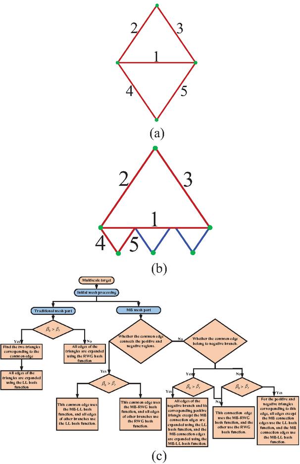
Figure 3 Specific replacement of the common edges corresponding to the basis function (a) when using the conformal mesh, (b) when using the nonconformal mesh, and (c) the implementation flowchart of the MB-LLB-AAE method.
In the case of using the nonconformal mesh, we need to calculate the angle between the positive triangle and each negative branch as , as shown in Fig. 2 (b).
Next, we need to presuppose a critical value . In the case of using a traditional conformal triangle, when corresponding to the common side is greater than , we replace the RWG basis functions corresponding to the common edge and the other four edges which belong to the positive and negative triangles of the common edge by the LL basis function (if the other common edge is open boundary, no replacement is done). Other common edges where is less than continue to be calculated using the RWG basis function. The specific replacement of the common edges corresponding to the basis function is shown in Fig. 3 (a). In the case of using nonconformal mesh, when the corresponding to the positive triangle and the negative branch is greater than , the MB-RWG basis function corresponding to this common edge is replaced with the MB-LL basis function. Then we replace the RWG basis functions corresponding to the other two common sides of the positive triangle and the RWG basis functions corresponding to the other two common edges of this negative branch with LL basis functions (if the other common sides are open boundaries, no replacement is made). The other common edges where is less than continue to use the RWG basis functions or the MB-RWG basis functions for calculation. The specific common edges corresponding to the replacement RWG basis function is shown in Fig. 3 (b). These are the construction rules of the AAE method. To facilitate readers’ understanding of the method, the implementation flowchart of the proposed algorithm is illustrated in Fig. 3 (c).
In actual engineering, only a few computational parts can be very sharp. As a result, the RWG-basis functions and the MB-RWG basis functions are still dominant, only in the sharp parts do we introduce the LL basis functions and the MB-LL-basis functions to improve calculation accuracy. Therefore, compared with using the LL basis functions and the MB-LL basis functions only for calculation, the AAE method can effectively reduce calculation consumption. At the same time, generally speaking, the sharp parts are the parts that need to be locally refined during our calculations. When using the MB method, a finer mesh can be used to calculate the sharp parts, and a coarser mesh can be used to calculate the smooth parts. This leads to a high possibility of mesh boundaries near the sharp parts. Therefore, it is meaningful to discuss the construction rules of the AAE method in the case of nonconformal meshes. We usually set to , which is enough to ensure the good performance of AAE.
4 NUMERICAL RESULTS
The platform used for performing the simulations is a workstation with a 32-core AMD Ryzen Threndripper Pro 3975 WX CPU@ 3.50 GHz and 512 GB RAM. All objects are illuminated by the plane wave propagating in direction, and the incident field is -polarized. The generalized minimum residual method (GMRES) is used to solve the matrix equation, and the residual is .
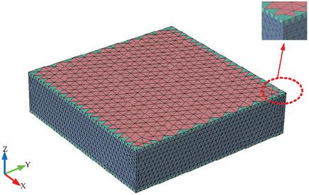
Figure 4 Mesh schematic diagram of PEC cube for MB method.
4.1 Cube
In the first example, we use a simple PEC cube model to verify the correctness and accuracy of the proposed algorithm. The size of this cube model is m. The center of the model is at the origin and its operating frequency is 300 MHz. To verify the advantage of the proposed method in terms of accuracy, we introduce relative error and define it as:
| (30) |
where represents the bistatic RCS result obtained by using a relatively fine mesh and the RWGEFIE method for calculation. Since the EFIE method was used and the mesh was relatively fine, the calculation result is relatively accurate. We take it as the reference standard. is the result of bistatic RCS calculated by six methods, namely MB-RWGCFIE method, MB-RWG-MFIE method, MB-LL-CFIE method, MB-LL-MFIE method, MB-AAE-CFIE method, and MB-AAE-MFIE method. For the EFIE method serving as the reference standard, we use triangles with an average side length of to perform meshing on the entire target. For the six methods, we use triangles with an average side length of to perform meshing on two faces of the cube model, and use triangles with an average side length of to perform meshing on the other four faces. The junctions of the different sizes mesh are connected using MB-RWG basis functions or MB-LL basis functions. For the MB-AAE-CFIE method and the MB-AAEMFIE method, we set to . We present the mesh diagram of the MB method in Fig. 4 and mark the parts in cyan of the AAE method where the MB-RWG basis functions need to be replaced with the MB-LL basis functions. It can be seen that only a small portion of the MB-RWG basis functions have been replaced with MBLL basis functions.
In Fig. 5 (a), we present a comparison chart of the relative error of the six methods. It can be seen that, compared with the MB-RWG-CFIE method and the MB-RWG-MFIE method, the other four methods effectively reduce the calculation error, and the improvement of accuracy by the method based on AAE is not much different from that of the method based on LL basis functions. To further verify the accuracy of the proposed method, we define the root-mean-square errors (RMSE) of the RCS as:
| (31) |
where . Ee use RCS results of and to calculate RMSE. The comparison of RMSE between the MB-RWG-CFIE method, the MB-LLCFIE method, and the MB-AAE-CFIE method are presented in Fig. 5 (b). It can be seen that the RMSE of both methods will gradually decrease with the increase of , and eventually converge to 0. However, the RMSE of MB-AAE-CFIE method is smaller than that of MB-RWG-CFIE method, and the convergence speed is faster than that of the MB-RWG-CFIE method, and is basically consistent with the MB-LL-CFIE method. Table 1 presents a comparison of the computational resource consumption between the MB-LL method and the MB-LLB-AAE method. It can be observed that, in comparison with the MB-LL method, the MB-LLBAAE method achieves a reduction of approximately 5% in the number of unknowns and a decrease of about 20% in computation time. This result preliminarily validates the superiority of the MB-LLB-AAE method in terms of computational resource savings.
4.2 Ship
In the second example, we use a complex multiscale ship model to verify the advantages of the proposed method in terms of accuracy and computing resource consumption. The ship model is 23.19 m in length, 2.52 m in width, 4.82 m in height, and operates at a frequency of 300 MHz. This ship model not only has a large-sized hull but also has small-sized naval guns, missile cabins, a cockpit, and high-power microwave weapons distributed on it.
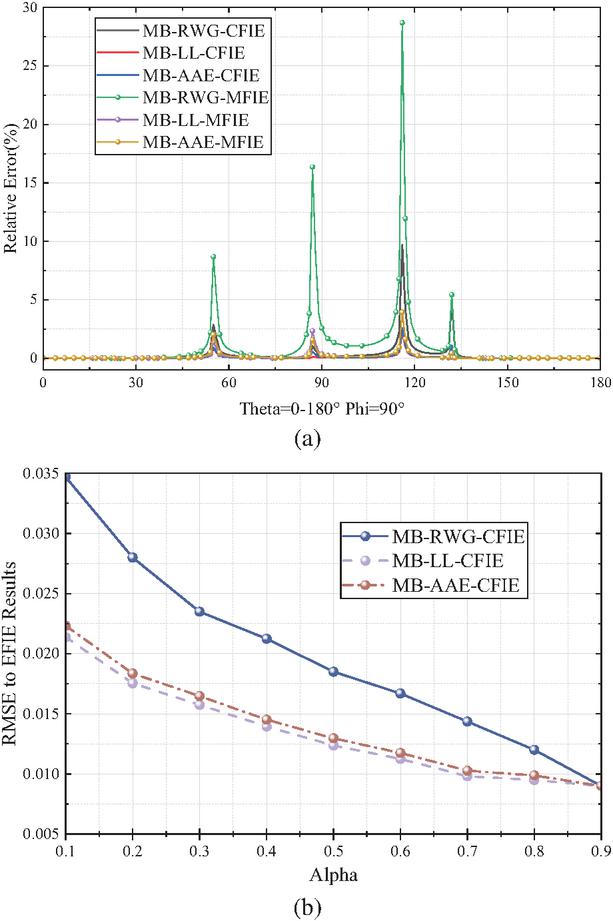
Figure 5 (a) Relative error of the six methods and (b) RMSE to EFIE results of the MB-RWG-CFIE method, MB-LL-CFIE method, and the MB-AAE-CFIE method.
Table 1 Calculation resource comparison of three methods for analyzing the PEC cube
| Method | Number of | Memory | CPU |
| Unknowns | of Z | Time | |
| MB-LL-CFIE | 7302 | 531 MB | 7.7 min |
| MB-AAE-CFIE | 6942 | 475 MB | 6.3 min |
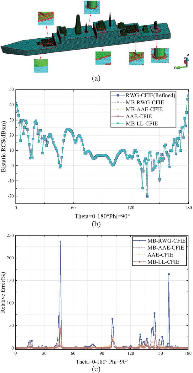
Figure 6 (a) Mesh schematic diagram of the PEC ship for MB method. (b) Bistatic RCS results for the PEC ship. (c) Relative error results of the MB-RWG-CFIE method, the MB-AAE-CFIE method, the AAE-CFIE method and the MB-LL-CFIE method for the PEC ship.
This ship model is a typically complex and practically significant multiscale model. For this ship model, we still first use the EFIE method that utilizes fine meshes for calculation and take the calculation results as the reference standard.
Table 2 Calculation resource comparison of three methods for analyzing the PEC ship
| Method | Number of | Memory | CPU |
| Unknowns | of Z | Time | |
| AAE-CFIE | 113452 | 126062 MB | 656.8 min |
| MB-LL-CFIE | 89502 | 78456 MB | 408.7 min |
| MB-AAE-CFIE | 50482 | 25416 MB | 132.6 min |
We use triangles with an average side length of to mesh the entire ship. Next, we use the AAECFIE method, MB-AAE-CFIE method, MB-LL-CFIE method and MB-RWG-CFIE method for calculation. For the MB method, we use a triangle with an average side length of to mesh the hull. The fine structure of the ship is meshed using triangles with an average side length of . The connection points of mesh of different sizes are connected using MB-RWG basis functions or MB-LL basis functions. For the AAECFIE method, the triangles with an average side length of are used to mesh the whole modal and selected at . In Fig. 6 (a), we present the mesh scheme of the MB method and mark the parts where the MB-RWG basis functions are replaced with the MB-LL basis functions in red.
In Fig. 6 (b), we present the RCS result of the above five methods. To show the accuracy differences more clearly, we present the relative errors of the other four methods and the control group (EFIE with fine mesh) in Fig. 6 (c). It can be seen that the relative error of the MB-AAE-CFIE method is not much different from that of the AAE-CFIE method and the MB-LL-CFIE method, and is much lower than that of the MB-RWG-CFIE method. Meanwhile, in Table 2, we compared the computational consumption of the MB-AAE-CFIE method, the AAE-CFIE method, and the MB-LL-CFIE method. It can be seen that the computational consumption of the MB-AAE-CFIE method is much lower than that of the other two methods in comparison with the MB-LL method, the MB-LLB-AAE method achieves a reduction of approximately 43% in the number of unknowns and a decrease of about 67% in computation time. The proposed method effectively reduces computational cost while improving accuracy, which is very significant for calculating large-scale targets.
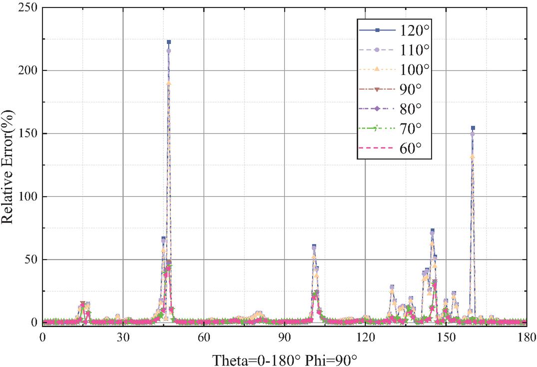
Figure 7 Comparison of relative errors for the MB-LLBAAE method with different angles.
Table 3 Comparison of computational resource consumption for the MB-LLB-AAE method with different angles for analyzing the PEC ship
| Number of | Reduction | |
| Unknowns | Percentage | |
| 44964 | 49.7% | |
| 45226 | 49.4% | |
| 45342 | 49.3% | |
| 50482 | 43.5% | |
| 50722 | 43.3% | |
| 50982 | 43.0% | |
| 51120 | 42.8% |
To justify the selection of as the criterion for parameter , a sensitivity study is performed in this work. The parameter is set to , , and , respectively, and all numerical tests are implemented using the MB-LLB-AAE method. The relative errors with respect to the dense-mesh RWGEFIE solution are depicted in Fig. 7, while the number of unknowns and the corresponding reduction percentages relative to the MB-LL method are summarized in Table 3.
It can be observed that, as decreases, the relative error declines gradually, whereas the number of unknowns increases and the reduction ratio decreases accordingly. A distinct turning point is observed at , where the relative error is notably reduced and the unknowns increase significantly. This phenomenon arises because enables the inclusion of right-angle structures, which are the most frequently encountered configurations in practical engineering applications. When exceeds , the variation in both accuracy and computational cost becomes relatively mild. Conversely, when is smaller than , typical rightangle edges cannot be covered, and only marginal accuracy improvement can be achieved at the expense of excessive computational resources.
Accordingly, is adopted as the standard value for , which achieves a favorable balance between improved accuracy and affordable computational overhead. In addition, only the ship model is employed for sensitivity analysis, since the cube model only contains right-angle edges and planar surfaces, which provides limited significance for validation. As a realistic engineering model, the ship model is more suitable to demonstrate the rationality of choosing as the criterion for .
5 CONCLUSION
In this paper, we propose a novel MB-AAE method for improving the accuracy of MFIE and CFIE. This method only needs to replace a small part of the RWG basic functions and the MB-RWG basic functions with the LL basic functions and the MB-LL basic functions to effectively improve the calculation accuracy. This gives this method an advantage in terms of computing resource consumption. At the same time, this method inherits the advantages of the MB method and can effectively connect mesh of different sizes which is of great significance for calculating multiscale targets. It should be emphasized that the MB-LLB-AAE method can maintain efficiency even when sharp features () account for more than 30% of the target. Furthermore, the proposed method can be extended to the computation of dielectric targets in the future to improve the calculation accuracy for dielectric objects. Therefore, the proposed method shows promising prospects in both application and development.
REFERENCES
[1] K. Majcher, M. Musiał, W. Pakos, and T. Trapko, “A systematic review of HPM energy absorbers for building applications,” Energies, vol. 14, no. 19, pp. 6061–6083, Sep. 2021.
[2] Q. Guo, J. Su, Z. Li, J. Song, and Y. Guan, “Miniaturized-element frequency-selective rasorber design using characteristic modes analysis,” IEEE Trans. Antennas Propag., vol. 68, no. 9, pp. 6683–6693, Sep. 2020.
[3] Q. Guo, Z. Li, J. Su, L. Y. Yang, and J. Song, “Dual-polarization absorptive/transmissive frequency selective surface based on tripole elements,” IEEE Antennas Wireless Propag. Lett., vol. 18, no. 5, pp. 961–965, May 2019.
[4] S. Rao, D. Wilton, and A. Glisson, “Electromagnetic scattering by surfaces of arbitrary shape,” IEEE Trans. Antennas Propag., vol. 30, no. 3, pp. 409–418, May 1982.
[5] P. Ylä-Oijala, M. Taskinen, and S. Järvenpää, “Surface integral equation formulations for solving electromagnetic scattering problems with iterative methods,” Radio Sci., vol. 40, no. 06, pp. 1–19, Dec. 2005.
[6] P. Yla-Oijala and M. Taskinen, “Well-conditioned Muller formulation for electromagnetic scattering by dielectric objects,” IEEE Trans. Antennas Propag., vol. 53, no. 10, pp. 3316–3323, Oct. 2005.
[7] W. C. Chew, Waves and Fields in Inhomogeneous Media. Berlin, Germany: Van Nostrand Reinhold, 1990, Reprinted by IEEE Press, 1995.
[8] W. C. Chew, C. Davis, K. Warnick and L. Gürel, “EFIE and MFIE, why the difference?” in Proc. IEEE Antennas Propag. Soc. Int. Symp. USNC/URSI Nat. Radio Sci. Meeting, San Diego, CA, USA, pp. 1–2, July 2008.
[9] P. Yla-Oijala and M. Taskinen, “Application of combined field integral equation for electromagnetic scattering by dielectric and composite objects,” IEEE Trans. Antennas Propag., vol. 53, no. 3, pp. 1168–1173, Mar. 2005.
[10] J. M. Rius, E. Ubeda, and J. Parrón, “On the testing of the magnetic field integral equation with RWG basis functions in method of moments,” IEEE Trans. Antennas Propag., vol. 49, no. 11, pp. 1550–1553, Nov. 2001.
[11] L. Gurel and O. Ergul, “Singularity of the magnetic-field integral equation and its extraction,” IEEE Antennas Wireless Propag. Lett., vol. 4, pp. 229–232, 2005.
[12] S. Yan, J.-M. Jin, and Z. Nie, “Improving the accuracy of the second-kind Fredholm integral equations by using the Buffa-Christiansen functions,” IEEE Trans. Antennas Propag., vol. 59, no. 4, pp. 1299–1310, Apr. 2011.
[13] O. Ergul and L. Gurel, “The use of curl-conforming basis functions for the magnetic-field integral equation,” IEEE Trans. Antennas Propag., vol. 54, no. 7, pp. 1917–1926, July 2006.
[14] E. Ubeda and J. M. Rius, “Novel monopolar MoM-MFIE discretization for the scattering analysis of small objects,” IEEE Trans. Antennas Propag., vol. 54, no. 1, pp. 50–57, Jan. 2006.
[15] O. Ergul and L. Gurel, “Solid-angle factor in the magnetic-field integral equation,” Microw. Opt. Technol. Lett., vol. 45, no. 5, pp. 452–456, June 2005.
[16] O. Ergul and L. Gurel, “Improving the accuracy of the MFIE with the choice of basis functions,” Proc. IEEE Antennas and Propagation Soc. Int. Symp., vol. 3, pp. 3389–3392, 2004.
[17] K. Cools, F. P. Andriulli, D. De Zutter, and E. Michielssen, “Accurate and conforming mixed discretization of the MFIE,” IEEE Antennas Wireless Propag. Lett., vol. 10, pp. 528–531, 2011.
[18] J. Kornprobst and T. F. Eibert, “An accurate low-order discretization scheme for the identity operator in the magnetic field and combined field integral equations,” IEEE Trans. Antennas Propag., vol. 66, no. 11, pp. 6146–6157, Nov. 2018.
[19] B. Karaosmanoğlu, C. Önol, and Ö. Ergül, “Optimizations of EFIE and MFIE combinations in hybrid formulations of conducting bodies,” Proc. Int. Conf. Electromagn. Adv. Appl., pp. 1276–1279, Oct. 2015.
[20] L. C. Trintinalia and H. Ling, “First order triangular patch basis functions for electromagnetic scattering analysis,” J. Electromagn. Waves Appl., vol. 15, no. 11, pp. 1521–1537, 2001.
[21] Y. Pan, X.-W. Huang, and X.-Q. Sheng, “A simple combined-field integral equation strategy for electromagnetic scattering from PEC objects,” IEEE Trans. Antennas Propag., vol. 69, no. 6, pp. 3611–3616, June 2021.
[22] Z. Peng, K.-H. Lim, and J.-F. Lee, “A discontinuous Galerkin surface integral equation method for electromagnetic wave scattering from nonpenetrable targets,” IEEE Trans. Antennas Propag., vol. 61, no. 7, pp. 3617–3628, July 2013.
[23] E. Ubeda, J. M. Rius, and A. Heldring, “Nonconforming discretization of the electric-field integral equation for closed perfectly conducting objects,” IEEE Trans. Antennas Propag., vol. 62, no. 8, pp. 4171–4186, Aug. 2014.
[24] L. Huang, H.-X. Zhang, Y. Liao, L. Zhou, and W.-Y. Yin, “Discontinuous Galerkin method using Laguerre polynomials for solving a time-domain electric field integral equation,” IEEE Antennas Wireless Propag. Lett., vol. 17, no. 5, pp. 865–868, May 2018.
[25] C.-B. Zhang and X.-Q. Sheng, “An efficient discontinuous Galerkin method for cavity design,” IEEE Antennas Wireless Propag. Lett., vol. 20, no. 2, pp. 199–203, Feb. 2021.
[26] S. Huang, G. Xiao, Y. Hu, R. Liu, and J. Mao, “Multibranch Rao-Wilton-Glisson basis functions for electromagnetic scattering problems,” IEEE Trans. Antennas Propag., vol. 69, no. 10, pp. 6624–6634, Oct. 2021.
[27] V. F. Martin, J. M. Taboada, and F. Vipiana, “A multi-resolution preconditioner for non-conformal meshes in the MoM solution of large multi-scale structures,” IEEE Trans. Antennas Propag., vol. 71, no. 12, pp. 9303–9315, Dec. 2023.
[28] Y. Wang, Y.-J. Zou, X.-J. Dang, M.-D. Zhu, and X.-W. Zhao, “A novel multibranch linear-linear basis function for improving the accuracy of multiscale PEC scattering analysis,” IEEE Antennas Wireless Propag. Lett., vol. 23, no. 2, pp. 748–752, Feb. 2024.
[29] M.-D. Zhu, T. K. Sarkar, Y. Zhang, and M. Salazar-Palma, “A novel framework of singularity cancellation transformations for strongly near-singular integrals,” IEEE Trans. Antennas Propag., vol. 69, no. 12, pp. 8539–8550, Dec. 2021.
BIOGRAPHIES
Yu Wang is a doctoral graduate from Xi’an University of Electronic Science and Technology, China. Currently, they work at the Key Laboratory of Advanced Science and Technology on High Power Microwave of Northwest Institute of Nuclear Technology, mainly engaged in research on electromagnetic calculation and electromagnetic compatibility.
Jie Cheng, doctor, studied at Xi’an Jiaotong University, China. Currently, they work at the Key Laboratory of Advanced Science and Technology on High Power Microwave of Northwest Institute of Nuclear Technology.
Yu Zhang is a doctoral graduate from National University of Defense Technology, China. Currently, they work at the Key Laboratory of Advanced Science and Technology on High Power Microwave of Northwest Institute of Nuclear Technology, mainly engaged in research on electromagnetic compatibility.
Lei Yu is graduate from Army Engineering University, China. Currently, they work at the Key Laboratory of Advanced Science and Technology on High Power Microwave of Northwest Institute of Nuclear Technology, mainly engaged in research on electrical system.
Liu-Yang Shen is a doctoral graduate from Lanzhou University, China. Currently, they work at the Key Laboratory of Advanced Science and Technology on High Power Microwave of Northwest Institute of Nuclear Technology, mainly engaged in research on ionization protection.
Sheng Liu is a doctoral graduate from Tsinghua University, China. Currently, they work at the Key Laboratory of Advanced Science and Technology on High Power Microwave of Northwest Institute of Nuclear Technology, mainly engaged in research on drive source technology.
ACES JOURNAL, Vol. 41, No. 5, 389–397
DOI: 10.13052/2026.ACES.J.410501
© 2026 River Publishers